
Graffiti of a zeolite (Photo taken from Mineralogisch ...
188
Graffiti of a zeolite (Photo taken from Mineralogisch-Petrologisches Institut und Museum der Universität Bonn, Poppelsdorfer Schloß, D-53115 Bonn).
Transcript of Graffiti of a zeolite (Photo taken from Mineralogisch ...

Graffiti of a zeolite (Photo taken from Mineralogisch-Petrologisches Institut und Museum derUniversität Bonn, Poppelsdorfer Schloß, D-53115 Bonn).

Theoretical Investigation of Static and Dynamic
Properties of Zeolite ZSM-5 Based Amorphous
Material
Inauguraldissertation zur Erlangung des Doktorgrades
der Mathematisch-Naturwissenschaftlichen Fakultät
der Universität zu Köln
vorgelegt von
Atashi Basu Mukhopadhyay
aus Kanchrapara
Köln 2004

Berichterstatter: Prof. Dr. M. DolgProf. Dr. U. K. Deiters
Tag der mündlichen Prüfung: 13.07.04
Acknowledgments
This thesis is the result of three years of work whereby I have been supported by many people.
It is a pleasant aspect that I have now the opportunity to express my gratitude for all of them.
The first person I would like to thank is my direct supervisor Prof. Dr. Michael Dolg. His
overly enthusiasm and integral view on research has made a deep impression on me. I owe him
lots of gratitude for being an excellent supervisor and a good friend.
I would like to thank my other supervisor Prof. Dr. Christina Oligschleger who kept an
eye on the progress of my work. I would like to thank Christa, for our many discussions and
providing me with suggestions and tips that helped me a lot in staying at the right track.
I would also like to thank the other members of my PhD committee Prof. Dr. U. K. Deiters
and Prof. Dr. U. Ruschewitz who took effort in reading and providing me with valuable
comments on this thesis.
I am grateful to Deutsche Forschungsgemeinschaft for financial support through SFB 408.
I thank the Forschungszentrum Jülich for generous grant of computer time on CRAY T3E
systems (Project No. k2710000).
I acknowledge the theoretical chemistry group at Köln for contribution to the development
of this work. Dr. Michael Hanrath helped me with the library routines for my programs. His
lectures and discussions on advanced quantum-chemical topics were quite informative. Dr.
Johannes Weber and Frau Birgitt Börsch-Pulm helped me with the computers. Dr. Xiaoyan
Cao gave a lot of suggestions which helped me to adjust to the new environment when I came
from India. I would like to thank my other colleagues, i.e., Mr. Martin Böhler, Ms. Rebecca
Fondermann, Mr. Sombat Ketrat, Mr. Joachim Friedrich, Mr. Jun Yang, Mr. Marc Burkatzki
and Mr. Alexander Schnurpfeil for providing friendly atmosphere in office.
I would like thank people at theoretical chemistry group, Bonn and specially for giving
me my favorite room as my office (facing towards east and with lots of sunshine) where I had
completed around 80% of my doctoral work before moving to Köln. I would like to thank Prof.
Dr. S. D. Peyerimhoff for providing intellectually stimulating atmosphere. Many thanks to Mr.
Jens Mekelburger for being patient with me and sorting out all computer related problems. I
would like to thank Dr. Bernd Nestmann and Prof. Dr. Miljenko Peric for being wonderful
friends. Special thanks to my other colleagues, i.e., Frau Claudia Kronz, Dr. Jan Franz, Mr.
Werner Reckien, Dr. Thomas Beyer, Dr. Boris Schäfer-Bung, Dr. Vincent Brems and Mr.
Jan Haubrich for making me feel at home at the institute. I would also like to thank my other
colleagues at FH Rhein-Sieg, Rheinbach.

Apart from work, special thanks to many of my friends at Bonn and NCL, Pune. I also
want to say thank-you to my parents and my brother for their understanding and faith in me.
Thanks to my in-laws for their support.
Last, but not the least, I would like to thank my husband Kausik for love, patience and
encouragement. Without your letters, mails and phone-calls I could not have survived these
three and a half years away from you.

My Family

Contents
1 Introduction 11.1 Amorphous Materials. . . . . . . . . . . . . . . . . . . . . . . . . . 21.2 Amorphous Materials Derived From Zeolite. . . . . . . . . . . . . . 4
1.2.1 Zeolites. . . . . . . . . . . . . . . . . . . . . . . . . . . . . 41.2.2 Zeolite-based amorphous materials. . . . . . . . . . . . . . 5
1.3 About this Work. . . . . . . . . . . . . . . . . . . . . . . . . . . . . 6
I Theoretical Background 9
2 Classical Molecular Dynamics 112.1 From the Schrödinger Equation to Classical Molecular Dynamics. . . 112.2 Equations of Motion . . . . . . . . . . . . . . . . . . . . . . . . . . 14
2.2.1 Lagrange equations of motion. . . . . . . . . . . . . . . . . 142.2.2 Hamilton equations of motion. . . . . . . . . . . . . . . . . 15
2.3 General Procedure for Molecular Dynamics. . . . . . . . . . . . . . 152.4 Interaction Potential. . . . . . . . . . . . . . . . . . . . . . . . . . . 16
2.4.1 Short-range potential. . . . . . . . . . . . . . . . . . . . . . 172.4.2 Long-range potential. . . . . . . . . . . . . . . . . . . . . . 20
2.5 Integrators. . . . . . . . . . . . . . . . . . . . . . . . . . . . . . . . 212.5.1 Verlet integrator . . . . . . . . . . . . . . . . . . . . . . . . 222.5.2 Leap Frog integrator. . . . . . . . . . . . . . . . . . . . . . 232.5.3 Velocity Verlet integrator. . . . . . . . . . . . . . . . . . . . 24
2.6 Simulations in Different Ensembles. . . . . . . . . . . . . . . . . . 242.6.1 Sampling from an ensemble. . . . . . . . . . . . . . . . . . 242.6.2 Common statistical ensembles. . . . . . . . . . . . . . . . . 252.6.3 Molecular dynamics at constant temperature. . . . . . . . . 272.6.4 Molecular dynamics at constant pressure. . . . . . . . . . . 30
2.7 Periodic Boundary Conditions. . . . . . . . . . . . . . . . . . . . . 32
i

ii CONTENTS
3 Large-Scale Optimization 353.1 Basic Approach to Large-Scale Optimization. . . . . . . . . . . . . 353.2 Basic Descent Structure of Local Methods. . . . . . . . . . . . . . . 373.3 Nonderivative Methods. . . . . . . . . . . . . . . . . . . . . . . . . 383.4 Gradient Methods. . . . . . . . . . . . . . . . . . . . . . . . . . . . 38
3.4.1 Steepest descent method. . . . . . . . . . . . . . . . . . . . 383.4.2 Conjugate gradient method. . . . . . . . . . . . . . . . . . . 403.4.3 Newton-Raphson method. . . . . . . . . . . . . . . . . . . . 42
4 Solid State Properties 454.1 Structural Properties. . . . . . . . . . . . . . . . . . . . . . . . . . 45
4.1.1 Diffraction by crystals . . . . . . . . . . . . . . . . . . . . . 454.1.2 Investigation of structures of non-crystalline solids. . . . . . 47
4.2 Vibrational Properties. . . . . . . . . . . . . . . . . . . . . . . . . . 494.2.1 Phonons. . . . . . . . . . . . . . . . . . . . . . . . . . . . . 494.2.2 Properties under harmonic approximation. . . . . . . . . . . 514.2.3 Anomalies in amorphous systems. . . . . . . . . . . . . . . 53
4.3 Elastic Constants. . . . . . . . . . . . . . . . . . . . . . . . . . . . 544.3.1 Elastic strains and stresses. . . . . . . . . . . . . . . . . . . 554.3.2 Stress components. . . . . . . . . . . . . . . . . . . . . . . 564.3.3 Elastic compliance and stiffness constants. . . . . . . . . . . 56
5 Quantum Chemical Treatment of Solids 595.1 Overview of Quantum Chemical Methods. . . . . . . . . . . . . . . 59
5.1.1 The Hartree-Fock method. . . . . . . . . . . . . . . . . . . 595.1.2 Electron correlation methods. . . . . . . . . . . . . . . . . . 605.1.3 Density functional theory. . . . . . . . . . . . . . . . . . . . 64
5.2 Ab Initio Treatment of Periodic System. . . . . . . . . . . . . . . . 665.2.1 The finite-cluster approaches. . . . . . . . . . . . . . . . . . 665.2.2 Bloch-orbital-based approach. . . . . . . . . . . . . . . . . 685.2.3 Wannier-orbital-based approach. . . . . . . . . . . . . . . . 69
II Applications 73
6 Structural Properties 756.1 Computational Details. . . . . . . . . . . . . . . . . . . . . . . . . 75
6.1.1 Interaction potential. . . . . . . . . . . . . . . . . . . . . . 756.1.2 Preparation of amorphous configurations. . . . . . . . . . . 76
6.2 Short-Range Order. . . . . . . . . . . . . . . . . . . . . . . . . . . 786.3 Connectivity of the Elementary Units. . . . . . . . . . . . . . . . . 796.4 Extent of Amorphization. . . . . . . . . . . . . . . . . . . . . . . . 86
CONTENTS iii
6.4.1 Defect in coordination number. . . . . . . . . . . . . . . . . 866.4.2 Internal surface area. . . . . . . . . . . . . . . . . . . . . . 896.4.3 Ring analysis. . . . . . . . . . . . . . . . . . . . . . . . . . 92
7 Vibrational Properties 977.1 Vibrational Density of States. . . . . . . . . . . . . . . . . . . . . . 977.2 Analysis of the Vibrational Modes. . . . . . . . . . . . . . . . . . . 101
7.2.1 Element specific motion with respect to bonds. . . . . . . . . 1017.2.2 Relative contribution of motions of structural subunits to DOS1027.2.3 Mode localization. . . . . . . . . . . . . . . . . . . . . . . . 1087.2.4 Phase quotient. . . . . . . . . . . . . . . . . . . . . . . . . 110
7.3 Effect of Extent of Amorphization on Vibrational DOS. . . . . . . . 1117.4 Low-Frequency Vibrational Excitations. . . . . . . . . . . . . . . . 113
8 Relaxation Properties 1218.1 Time Evolution on the Energy Landscape. . . . . . . . . . . . . . . 1238.2 Structure and Mode of Relaxations. . . . . . . . . . . . . . . . . . . 1238.3 Correlation between Jumps. . . . . . . . . . . . . . . . . . . . . . . 1288.4 Heterogeneity. . . . . . . . . . . . . . . . . . . . . . . . . . . . . .129
9 Two-Fold Rings in Silicates 1339.1 Applied Methods and Technical Details. . . . . . . . . . . . . . . . 135
9.1.1 Finite-Cluster approach/A simple approach. . . . . . . . . . 1369.1.2 Incremental approach. . . . . . . . . . . . . . . . . . . . . . 136
9.2 Structure and Stability of Two-Fold Ring. . . . . . . . . . . . . . . . 137
10 Summary and Outlook 145
References 149
Abstract 161
Kurzzusammenfassung 163
List of Publications 165
Lebenslauf 167
Erklärung 169

List of Figures
1.1 P, T diagram of ordered and disordered states of a typical pure com-pound. . . . . . . . . . . . . . . . . . . . . . . . . . . . . . . . . . 2
1.2 Path of formation of vitreous and amorphous solids.. . . . . . . . . . 3
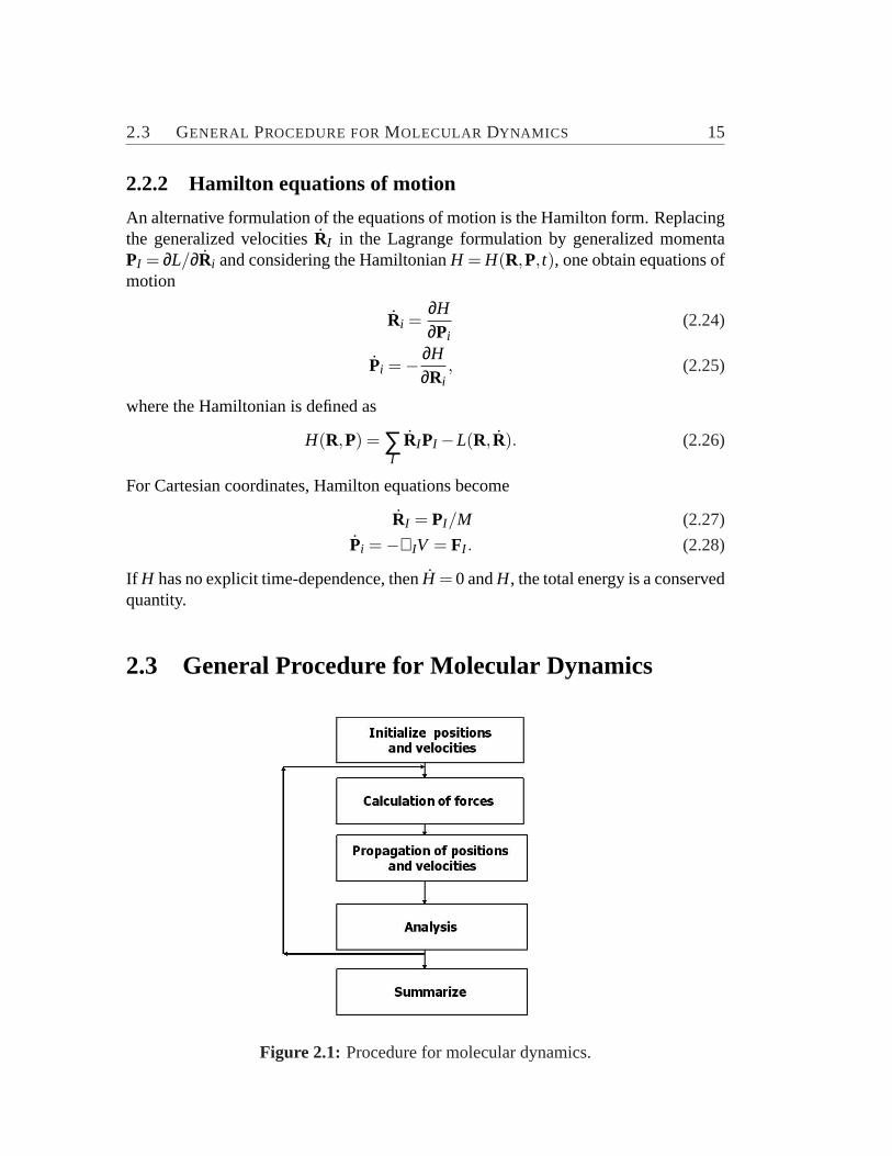
2.1 Flow chart of a MD program. . . . . . . . . . . . . . . . . . . . . . 15
3.1 The method of steepest descent.. . . . . . . . . . . . . . . . . . . . 393.2 The method of conjugate directions.. . . . . . . . . . . . . . . . . . 41
4.1 The Brillouin zones for a two-dimensional square lattice.. . . . . . . 494.2 Phonon dispersion relation.. . . . . . . . . . . . . . . . . . . . . . 51
6.1 Zeolite ZSM-5 viewed along y-axis.. . . . . . . . . . . . . . . . . . 776.2 Total and pair-distribution function.. . . . . . . . . . . . . . . . . . 826.3 Bond angle distribution. . . . . . . . . . . . . . . . . . . . . . . . . 836.4 Model for the connectivity of tetrahedra.. . . . . . . . . . . . . . . 846.5 Cross section of ZSM-5 (crystalline) and its amorphous derivatives.. 876.6 Distribution of coordination numbers of O and Si atoms.. . . . . . . 886.7 Internal surface area vs. percentage of energy crystallinity.. . . . . . 906.8 Distribution of ringsize. . . . . . . . . . . . . . . . . . . . . . . . . 93
7.1 Vibrational density of states of zeolite-based amorphous structure.. . 997.2 Averaged element specific-contribution to the total vibrational DOS.. 1017.3 The specific heat versus the temperature.. . . . . . . . . . . . . . . 1027.4 Distribution of element-specific weighted-average angles between the
atomic displacement eigenvectors and the bonds.. . . . . . . . . . . 1057.5 The total and partial vibrational DOS obtained by the projection of
the relative atomic displacements onto the vibrational vectors of theSi-O-Si and SiO4 subunits. . . . . . . . . . . . . . . . . . . . . . . . 107
7.6 Participation ratios of the crystalline and amorphous systems.. . . . 1097.7 Radius of gyration versus frequency .. . . . . . . . . . . . . . . . . 1107.8 Weighted phase quotient verses frequency.. . . . . . . . . . . . . . 1117.9 Vibrational DOS for different PEC versus frequency.. . . . . . . . . 112
v
vi L IST OF FIGURES
7.10 Reduced DOS and maximum of Reduced DOS for ZSM-5-based par-tially amorphous structures.. . . . . . . . . . . . . . . . . . . . . . 114
7.11 Phonon dispersion curves for the silicious ZSM-5.. . . . . . . . . . 1157.12 The active atoms of the modes of BP region.. . . . . . . . . . . . . 1187.13 Participation ratios of modes in BP region.. . . . . . . . . . . . . . 119
8.1 Element-specific diffusion constants.. . . . . . . . . . . . . . . . . 1228.2 Changes in the potential energy and displacement per atom during ag-
ing. . . . . . . . . . . . . . . . . . . . . . . . . . . . . . . . . . . .1248.3 Participation ratios against jump distance at different temperatures.. 1258.4 The dimensions of the jumps.. . . . . . . . . . . . . . . . . . . . . 1268.5 The distribution of correlations between the successive jumps at dif-
ferent temperature.. . . . . . . . . . . . . . . . . . . . . . . . . . .1288.6 Element-specific plot of the van Hove correlation functions.. . . . . 1308.7 The non-Gaussianity parameter for Si and O.. . . . . . . . . . . . . 131
9.1 Model of W-silica. . . . . . . . . . . . . . . . . . . . . . . . . . . .1349.2 Variation in the potential energy surface with respect to the area ofa-b
plane. . . . . . . . . . . . . . . . . . . . . . . . . . . . . . . . . . .1359.3 Convergence of the cohesive energy per Si2O4 unit of W-silica. . . . 1389.4 Convergence of the lattice parameter and Si-O distance of W-silica.. 1409.5 Finite clusters of a chain of W-silica andα-quartz. . . . . . . . . . . 141
List of Tables
6.1 Force-field parameters for BKS potential.. . . . . . . . . . . . . . . 766.2 Bond distances and bond angles for the bridged unit in edge-shared
SiO4 tetrahedra. . . . . . . . . . . . . . . . . . . . . . . . . . . . . 856.3 Atomic/ionic radii for O and Si depending on the coordination number.896.4 Ring analysis for ZSM-5 based amorphous material.. . . . . . . . . 94
7.1 Vibrational vectors for Si-O-Si subunits assuming O at rest.. . . . . 1037.2 Vibrational vectors for SiO4 subunits assuming Si at rest.. . . . . . . 1047.3 Partial contributions of the eigenmodes of the Si-O-Si and SiO4 sub-
units. . . . . . . . . . . . . . . . . . . . . . . . . . . . . . . . . . .1087.4 Ring analysis, degree of puckering and participation ratios of modes
for ZSM-5 based amorphous material.. . . . . . . . . . . . . . . . . 1167.5 Distribution of the CNs for the 10 % most active atoms in BP region.1177.6 Contributions of the vibrational motions exhibited by the active sub-
unit. . . . . . . . . . . . . . . . . . . . . . . . . . . . . . . . . . . .120
8.1 The average dimensionalities and average radii of gyration.. . . . . 1268.2 Relaxation with respect to bond changes.. . . . . . . . . . . . . . . 1278.3 Contributions of the relaxations exhibited by Si-O-Si and SiO4 sub-
units by the projectional analysis.. . . . . . . . . . . . . . . . . . . 127
9.1 Geometries of two-membered rings in W-silica.. . . . . . . . . . . . 1399.2 Increments to the correlation energy per unit cell.. . . . . . . . . . . 1429.3 Cohesive energies per SiO2 unit in α-quartz. . . . . . . . . . . . . . 1429.4 Relative energy of a Si2O4 unit with respect toα-quartz. . . . . . . . 143
vii

Abbreviations
AO Atomic Orbitala.u. Atomic UnitBF Bloch FunctionBKS Beest, Kramer and van SantenBP Boson PeakBZ Brillouin ZoneCC Coupled ClusterCCSD Coupled Cluster with Single and Double excitationsCI Configuration InteractionCISD Configuration Interaction truncated to Singles and Doubles substitutionCN Coordination NumberCO Crystal OrbitalsDFT Density Functional TheoryDOS Density of StatesFCI Full Configuration Interactionfs FemtosecondGGA Generalized Gradient ApproximationGTF Gaussian Type FunctionFWHM Full Width at the Half MaximumHF Hartree-FockIR InfraredISA Internal Surface AreaKS Kohn-ShamLDA Local Density ApproximationMC Monte CarloMD Molecular DynamicsMP Møller-PlessetNGP Non-Gaussianity Parameterns NanosecondPBC Periodic Boundary ConditionPEC Percentage of Energy Crystallinityps Picosecond
ix

x ABBREVIATIONS
QM/MM Quantum Mechanics and Molecular MechanicsRDF Radial Distribution FunctionRSPT Rayleigh-Schrödinger Perturbation TheoryTDSCF Time-Dependent Self-Consistent FieldTHz Terra HertzSCF Self-Consistent-FieldSDCG Steepest-Descent-Conjugate-GradientXRD X-Ray Diffractogram
Chapter 1
Introduction
“Amorphous materialper se, are not new:the iron-rich silicious glassy materials re-covered from the moon by the Apollomissions are some billions of years old,and man has been manufacturing glassymaterials for thousands of years. Whatis new, however is thescientific studyofamorphous materials and there has beenan explosion of interest recently as morenew materials produced in an amorphousform, some of which have considerabletechnological promise.”S. R. Elliott,Physics of Amorphous Ma-terials (1984).
1
2 CHAPTER 1 INTRODUCTION
1.1 Amorphous Materials
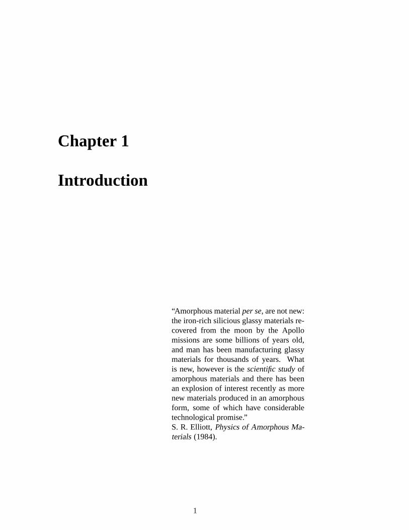
"Amorphous" meaning "structureless" describes all those states of matter whose prop-erties do not show a preferential direction unlike crystals. The range of disorderedstructures is far wider than that of crystalline phases, as seen from Fig.1.1 (repre-senting a phase diagram of a typical pure compound). By increasing pressure andtemperature under conditions which sufficiently delay spontaneous transition into thecrystalline state, amorphous solids can be continuously transformed into melts, andthe latter can further be transformed into the gaseous state if the critical temperature isexceeded. It is not possible, however to change from the ordered crystalline phase toone of the disordered states of aggregation without provoking discontinuous variationof certain variables of state, such as volume, enthalpy or entropy.
Figure 1.1: P, T diagram of ordered and disordered state of a typical pure compound
(Adapted from Ref. [2]).
The methods of X-ray, neutron and electron diffraction are helpful in distinguish-ing the amorphous substances from those that are crystalline. Instead of the distinctdiscrete diffraction maxima occurring for crystalline substances, only a few circularfringes are observed in amorphous solids. These circular fringes indicate a non-randomdistribution of interatomic distances, in other words, a degree of order that has beencarried over to the amorphous state. Hence, amorphous substances, like crystals, areusually characterized by certain areas ofshort-range order. These often correspondto the structural units of crystalline states, or at least are associated with them througha clear relationship in terms of chemical structure. As distance increases, the diver-sity of structural configurations also increases rapidly owing to a certain variablity inbond lengths, and especially in bond angles mainly due to the twisting of units rela-tive to each other, through partial rotation about the axes of chemical bonds. Hence, along-range order, as in crystals, does not exist in amorphous substances.
1.1 AMORPHOUSMATERIALS 3
The world ofquasi-crystallinesolids occupies a position between crystalline andamorphous matter. These materials seem to represent a fundamentally different phaseof solids, exhibiting symmetries that are impossible for ordinary solids. They ex-hibit the long-range orientational order rather than the translational one. This quasi-periodicity leads to well-defined X-ray diffraction pattern.
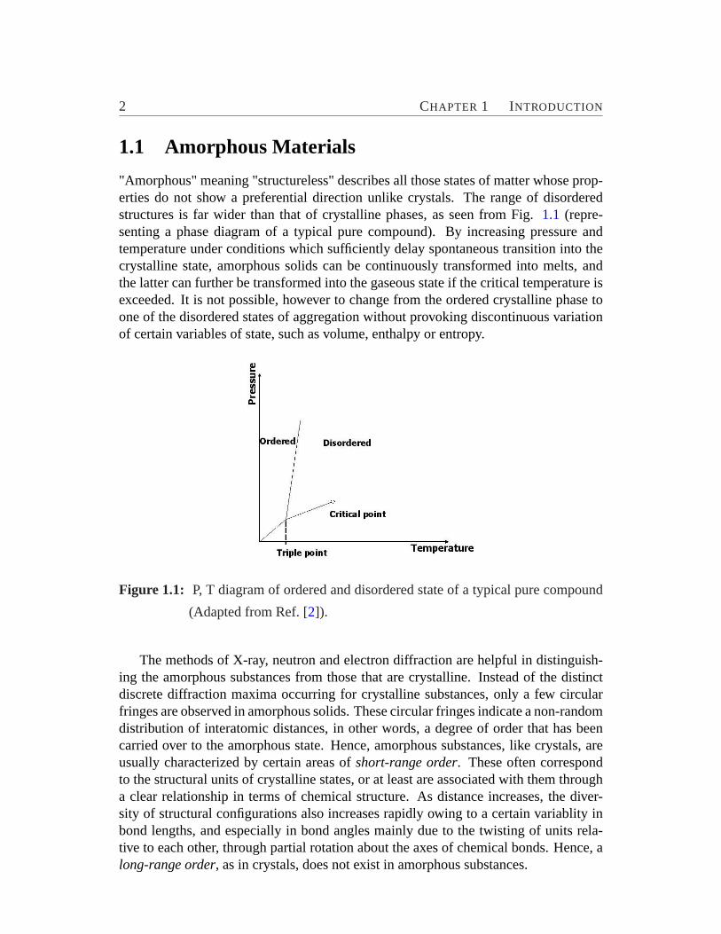
Figure 1.2: Path of formation of vitreous and amorphous solids from melts or solu-
tion, vapors and crystalline states of substances (Adapted from Ref. [2]).
Amorphous solids can be obtained from the liquid state, i.e., from a melt or solu-tion, or from the gas phase, provided that the formation of a periodic arrangement ofunits through the process of nucleation and crystallization is prevented. On the otherhand , by supplying energy to crystalline solids they can be converted to the amorphousstate directly without passing through the liquid or gaseous phases. A collection of themethods are summarized in Fig.1.2. Refer to Ref. [1,2] for further details. Glasses,a special class of non-crystalline solids, are obtained by sufficiently rapid quenchingof melts [3,4,5] or by drying of gels from solutions [6]. The process of precipitationof solutions often leads to amorphous precipitates [7]. Electrolytic separation usinga high current density also gives rise to the formation of amorphous layers [8]. Withregards to the methods starting from the gaseous phase, the most important of theseare thermal evaporation and condensation in high vacuum [9], cathode sputtering [10]and deposition of amorphous layers in chemical and glow discharge processes [11].Amorphous films or layers can also be generated by direct oxidation of crystals at thesurface [12]. Crystalline solids are also converted to amorphous solids by the influence

4 CHAPTER 1 INTRODUCTION
of mechanical treatment [13], shock waves [14] or intense radiation with neutrons orions [15].
1.2 Amorphous Materials Derived From Zeolite
1.2.1 Zeolites
The wordzeoliteis Greek in origin, coming from the words "zein" and "lithos" mean-ing to boil and rock. It was first used by the Swedish chemist and mineralogist A. F.Cronstedt in his paper announcing the discovery of a new class of tectosilicates [16].There was little interest in zeolites until the late 1930’s when the modern founderof zeolite chemistry, R. M. Barrer began the characterization of zeolite structure andchemistry [17]. His work gave details of the first method of laboratory synthesis ofzeolites from silicate alumina gels, the changes that occur upon ion exchange and theiruse as environmental friendly, shape selective catalysts. These discoveries sparkedhuge interest in the synthesis of shape selective zeolite catalysts in companies such asUnion Carbide and Mobil.
Chemically, zeolites are microporous solid-state crystalline materials having chan-nels, cages and windows of molecular dimensions. The zeolite framework consists ofan infinite array of corner-sharing TO4 tetrahedra. The tetrahedral atom T can be awide range of combinations of elements, e.g., Si and Al, B and Si, Ga and Si, etc. Incases where the T atoms cause a charge imbalance in the system, the charge neutralityis maintained by the incorporation of protons or extra-framework cations. The cationsusually occupy sites of relatively low coordination number in the structure and as aconsequence, are easy to ion-exchange. Although the tetrahedra are quite rigid, thereis considerable flexibility in the bond angles about the O atom (bond angle ranges from125◦ to close to 180◦ throughout the many known zeolite structures).
Zeolites are normally synthesized hydrothermally from basic reaction gels at tem-peratures between 60◦C and 200◦C under an autogenous pressure. Most of the highlysiliceous zeolites are formed in the presence of organic bases known as templates,introduced in the early 1960’s [18]. These ranges from simple hydrated cations tocomplex organic amines and crown ethers.
Due to their unique porous properties, zeolites are used in a variety of applications,with a global market of several million tons per annum. Following lists main applica-tions of zeolites.(i) Heterogenous catalysis: One of the most important applications of zeolites is inthe field of industrial catalysis. There are several factors which dictate the catalyticproperties of zeolites. Firstly, their large internal surface area (typically 300-700 m2/gor more than 98% of the total surface area) provides a high concentration of activesites, usually the Brønsted acid sites found in protonated zeolites. These are generallylocated as bridging hydroxyl group. The high thermal stability of many zeolite struc-
1.2 AMORPHOUSMATERIALS DERIVED FROM ZEOLITE 5
tures makes them ideal for use in an industrial environment where many processesoperate in conditions of high temperature and pressure. The shape selective propertiesof zeolites also control the results of many reactions inside the pore, either by allowingreactant or product molecules to selectively diffuse through the channels, or by thestabilization of the transition states.(ii) Adsorption and separation: The shape-selective properties of zeolites are also thebasis for their use in molecular adsorption. The ability preferentially to adsorb certainmolecules, while excluding others, has opened up a wide range of molecular siev-ing applications. The size and shape of pores and also chemical nature of diffusingmolecules control the access into the zeolite, e.g., as in the purification ofpara-xyleneby silicalite. Cation-containing zeolites are extensively used as desicants due to theirhigh affinity for water. These also find application in gas separation, where moleculesare differentiated on the basis or their electrostatic interactions with the metal ions.(iii) Ion exchange: The presence of loosely bound extra-framework cations in the ze-olite structure allows efficient ion exchange to occur in aqueous solution. This isexploited in many commercial applications. For example, Na Zeolite-A is used tosoften water by exchanging Na+ from the zeolite with Ca2+ in hard water. This is alsoa major component of concentrated washing powder formulations, where it replacessodium tripolyphosphate to reduce the environmentally hazardous phosphate concen-tration. Another important use of zeolites as ion-exchangers has been as radioactivedecontaminants. Clinoptilolite, for example, was used extensively after the Chernobylnuclear disaster to absorb radioactive ions such as90Sc and137Cs from the water sup-ply.
1.2.2 Zeolite-based amorphous materials
Zeolites undergo amorphization by mechanical [19, 20], high-pressure [21] and ther-mal [22] treatments. They also become amorphous when they are exposed to high-radiation doses and electron irradiation [23, 24]. Zeolite-based amorphous materialsare also proposed to be important for technological applications.
In order to quantify extent of amorphization, experimentalist use the percentageof X-ray diffractogram (XRD) crystallinity [28] based on the ratio of the major peakintensities of the sample relative to those of a highly crystalline reference material, i.e.,
% XRD crystallinity=sum of peak intensities of sample
sum of peak intensities of reference×100. (1.1)
Pore size and shape, Si/Al ratio or other modifications such as extra-frameworkcation exchange, isomorphous substitution, pore blockage, elimination of external sitesetc., are varying parameters for determining the product selectivity of zeolitic cataly-sis [26]. One of the reactions that has received considerable attention over the lastdecade is the skeletal isomerization of 1-butene to yield isobutene. The interest inthis reaction arises from the fact that the branched alkene can subsequently be reacted

6 CHAPTER 1 INTRODUCTION
with methanol for the synthesis of methyl-tertiary-butyl ether [27]. It was shown thatZSM-5 and ferrierite-based ZSM-5 materials with XRD crystallinity level as low as2% exhibited superior catalytic performance (higher selectivities and yields) in thisskeletal isomerization reactions compared to their conventional highly crystalline ana-logue. This was attributed to be a consequence of decreased zeolite pore lengths thatare presumably present in these amorphous materials [28]. Another industrially rele-vant reaction is the conversion of light alkanes into aromatic compounds which offersa useful route into high octane fuels [29,30]. ZSM-5 type materials have been used forthis type of reactions [31]. Recently, Zn and Ga incorporated novel aluminosilicates,comprising ZSM-5-based structures having XRD crystallinities ranging from substan-tially amorphous (XRD crystallinity lower than 30%) to the partially crystalline (XRDcrystallinity between 30% and 70%) and their highly crystalline (XRD crystallinityhigher than 70%) ZSM-5 analogues were studied [25]. Experiments show that the op-timum activity and the BTX (benzene, toulene and xylenes) selectivity are found forXRD crystallinity in the range 50%-85%.
Reversible cation exchange property is the basis for using zeolites in the selectiveremoval of radionuclides from high-level liquid nuclear waste. Amorphous forms de-rived from zeolites are proposed to be better back fill material for heavy metals [24].For example, amorphized zeolite Na-Y loses approximately 95% of its ion exchangecapacity for Cs due to loss of exchangeable cation sites and/or blockage of access toexchangeable cation sites. The Cs-exchanged zeolite Na-Y phase has a slightly higherthermal stability than the unexchanged zeolite Na-Y. A desorption study indicated thatthe amorphization of Cs loaded Na-Y zeolite enhances the retension capacity of ex-changeable Cs ions due to closure of structural channels.
1.3 About this Work
This thesis deals with the simulation of amorphous forms derived from zeolite. Exper-imental studies of mechanical treatment on zeolites show that amorphization causesremarkable changes in vibrational IR spectra and XRDs [19,20]. This implies that theamorphization process, i.e, the transformation from long-range to short-range orderingof the framework, is caused by structural changes at the molecular level. Thus, studiesof structural and dynamic aspects in these amorphous zeolite-based systems and theircorrelation to microscopic properties presents a fascinating challenge. Hence, under-standing the dependence of physical and chemical properties on the microstructure iscritical for designing new materials suitable for specific applications.
This work features as one of the projects under Sonderforschungsbereich 408 at theUniversity of Bonn, which deals with the investigation of structure and properties ofinorganic amorphous materials. All silica ZSM-5, i.e.,silicalite was chosen as a modelsystem for the preparation of the amorphous state, since it is experimentally a wellstudied system. Details of structure of zeolite silicalite (silicious ZSM-5) is presented

1.3 ABOUT THIS WORK 7
in chapter 6 (section 6.1.2). Despite of the significant interest of chemists to investigatethe chemical properties of the zeolite ZSM-5-based amorphous materials [28,25], theinvestigation of detailed structural and dynamic properties are lacking. To the best ofour knowledge this work is the first theoretical investigation on these lines.
The derivation of a detailed microscopic structure of any non-crystalline systemrepresent a big scientific challenge even today. Special experimental techniques needto be employed. Even when such techniques are used, only a limited amount of localstructural information is generally obtainable, and the construction of structural mod-els can be a most useful route to a further understanding of the structure, particularlythe medium-range order. The absence of translational symmetry and the requirementto treat rather large model clusters cut out from the infinite system makes the studyof amorphous materials using the availableab initio methods of quantum chemistryand solid state physics a very difficult, if not an unmanageable task. Whereas theseapproaches rely on the finite or periodic character of the investigated systems, a largenumber of real systems does not fall into these two categories but rather shows only apartially crystalline or even completely amorphous character. In such cases simulationtechniques like molecular dynamics (MD) and Monte Carlo (MC) have become widelyused tools to explore complicated amorphous systems. MC methods are applied to ex-plore configuration space, i.e, to search for minimum energy structures and to establishtheir properties as well as to study relaxation from a global point of view. However,sometimes the move-classes may be unphysical and do not give reliable insight intothe microscopic dynamics of the systems. MD is widely used to construct models ofthe amorphous state by rapid quenching of structures at high temperature and analyz-ing the dynamics of the model on a microscopic scale. The success of MD dependscrucially on the quality of the interaction potentials used to determine the energy andthe forces between interacting particles. The advantage of MD over MC is that it givesa route to study dynamic properties of systems.
In this thesis we have studied the structural (chapter 6) and dynamic (vibrationsand relaxations, chapter 7& 8) properties mainly on the basis of MD simulations. Oursimulations show presence of small percentage of edge-sharing connectivity of SiO4
tetrahedra depending on the extent of amorphization. We used wavefunction-basedabinitio methods for determining stability and structure of these unusual features (chapter9). We choose W-silica as a model system for edge-sharing tetrahedra silicate systemand compared our results with existing theoretical results.
The organization of the thesis is as follows:
• Part I: Theoretical Background−→ Basics of MD, local-optimization methods,modeling of solid-state and electron-correlation treatment of solid-state as needed incontext of this thesis.• Part II: Applications−→ Results concerning structural, vibrational and relaxationalproperties of amorphous form derived from zeolite ZSM-5.

Part I
Theoretical Background
9

Chapter 2
Classical Molecular Dynamics
2.1 From the Schrödinger Equation to Classical Molec-
ular Dynamics
The dynamical evolution of the wavefunction with time is given by thetime-dependentSchrödinger equation:
i~∂∂t
Φ({r i},{RI}; t) = HΦ({r i},{RI}; t) (2.1)
in its position representation with the standard non-relativistic Hamiltonian,
H =−∑I
~2
2MI∇2
I −∑i
~2
2me∇2
i + ∑i< j
e2
|r i− r j | −∑I ,i
e2ZI
|RI − r i | + ∑I<J
e2ZIZJ
|RI −RJ| (2.2a)
=−∑I
~2
2MI∇2
I −∑i
~2
2me∇2
i +Vn−e({r i},{RI}) (2.2b)
=−∑I
~2
2MI∇2
I +He({r i},{RI}) (2.2c)
for electronic and nuclear degrees of freedom. The total wave functionΦ({r i},{RI}; t)depends onRI andr i , the nuclear and electronic coordinates, respectively. An elegantderivation of the classical molecular dynamics derived by Tully [32,33,34] is presentedbelow. In order to separate the nuclear and electronic contributions to the wavefunctiona product ansatz
Φ({r i},{RI}; t)≈Ψ({r i}; t)χ({RI}; t)exp[ i~
Z t
t0dt′Ee(t ′)
](2.3)
11

12 CHAPTER 2 CLASSICAL MOLECULAR DYNAMICS
is introduced, where the nuclear and the electronic wavefunctions are separately nor-malized to unity at every instant of time.
Inserting the ansatz Eq. (2.3) into Eq.(2.1) yield (after multiplying from the left by〈Ψ| and〈χ| and imposingd〈H〉/dt ≡ 0) the following equations,
i~∂Ψ∂t
=−∑i
~2
2me∇2
i Ψ+{Z
dRχ∗({RI}; t)Vn−e({r i},{RI})χ({RI}; t)}
Ψ (2.4)
i~∂χ∂t
=−∑I
~2
2MI∇2
I χ+{Z
drΨ∗({r i}; t)He({r i},{RI})Ψ({r i}; t)}
χ. (2.5)
Eq. (2.4) and Eq. (2.5) are the basic equations of the mean-field time-dependent self-consistent field (TDSCF) method, where the fast moving electrons move in an averagefield of the slow moving nuclei andvice versa.
Following Messiah, the nuclear wavefunction can be factored into amplitude andphase terms,
χ({RI}; t) = A({RI}; t)exp[iS({RI}; t)/~] (2.6)
whereA andSare real-valued [35]. Substituting Eq. (2.6) into Eq. (2.5) and separatingthe real and imaginary parts, the TDSCF equation for nuclei becomes
∂A∂t
+∑I
12MI
(∇IA)(∇IS)+∑I
12MI
A(∇IS)2 = 0 (2.7)
and
∂S∂t
+∑I
12MI
(∇IS)2 +Z
drΨ∗HeΨ = ~2∑I
12MI
∇IAA
. (2.8)
Eq. (2.7) describes the flow of probability on the potential energy surface determinedby the velocity field∇IS. For the derivation of classical molecular dynamics considerEq. (2.8). In the classical limit this becomes
∂S∂t
+∑I
12MI
(∇IS)2 +Z
drΨ∗HeΨ = 0. (2.9)
Eq. (2.9) is known as quantum Hamilton-Jacobi equation, which is identical to theequation in Hamilton-Jacobi formulation of classical mechanics [35,36]
∂S∂t
+H({RI},{∇IS}) = 0 (2.10)
with the classical Hamilton function
H({RI},{PI}) = T({PI})+V({RI}) (2.11)
2.1 FROM THE SCHRÖDINGEREQUATION TO CLASSICAL MOLECULAR
DYNAMICS 13
defined in terms of generalized coordinates{RI} and their conjugate momenta{PI}.T andV refer to the classical kinetic energy and the potential energy, respectively.S(t)is the ’classical action’, i.e.,S(t) =
R t L(t ′)dt′ and
PI ≡ ∇IS, (2.12)
whereL(t ′) is the classical Lagrangian. Considering the Newtonian equation of motionPI =−∇IV({RI}), the Eq. (2.9) becomes
dPI
dt=−∇I
ZdrΨ∗HeΨ (2.13)
or
MI RI (t) =−∇I
ZdrΨ∗HeΨ (2.14)
=−∇IVEe ({RI (t)}). (2.15)
Thus the nuclei move according to the classical mechanics in an effective potentialVEe
due to electrons and its motion is a function of only the nuclear positions at timet.However the nuclear wavefunction still occurs in the TDSCF equation for the elec-
tronic degrees of freedom. In the classical limit Eq. (2.4) becomes a time-dependentwave function for the electrons
i~∂Ψ∂t
=−∑i
~2
2me∇2
i Ψ+Vn−e({r i},{RI})Ψ (2.16)
= He({r i},{RI})Ψ({r i},{RI}; t) (2.17)
which evolve self-consistently as the classical nuclei are propagated via Eq. (2.14).The approach relying on solving Eq. (2.14) together with Eq. (2.17) is calledEhrenfestmolecular dynamics.
A further simplification can be invoked by restricting the wavefunctionΨ to be theground state wavefunctionΨ0 of He at each instant of time. In this limit the nucleimove according to Eq. (2.14) on a Born-Oppenheimer potential energy surface
VEe =
ZdrΨ∗
0HeΨ0≡ E0({RI}) (2.18)
which can be obtained by solving thetime-independentelectronic Schödinger equation
HeΨ0 = E0Ψ0, (2.19)
for the ground state only.To perform classical trajectory calculations on the global potential energy surface,
it is conceivable to decouple the task of generating the nuclear dynamics from the taskof generating the potential energy surface. In a first stepE0 is computed for manynuclear configurations by solving Eq. (2.19). In a second step, these data points are

14 CHAPTER 2 CLASSICAL MOLECULAR DYNAMICS
fitted to an analytical functional form to yield a global potential energy surface [37],from which analytical gradients can be obtained. In the third step, the Newtonianequation of motion Eq. (2.15) is solved on this surface for many different initial con-ditions. However, calculation of the global potential energy surface is the limiting stepfor large systems. There are3N−6 internal degrees of freedom that span the globalpotential energy surface of an unconstrained N-body system. Using for simplicity10 discretization points per coordinate implies that of the order of103N−6 electronicstructure calculations are needed. Thus, computational workload increases roughlylike ∼ 10N with increasing system size. This is also referred to as thedimensionalitybottleneckof calculations that rely on global potential energy surfaces [38]. One tra-ditional way out of this dilemma is to approximate the global potential energy surface
VEe ≈V = Vapprox
e ({RI}) =N
∑I
υ1({RI})+N
∑I<J
υ2({RI ,RJ})+ · · · (2.20)
in terms of a truncated expansion of many-body contributions [39, 40]. Hence, theelectronic degrees of freedom are replaced by the interaction potentialsυn and are notfeatured as explicit degrees of freedom in the equations of motion. From the abovederivation the essential assumption underlying the classical molecular dynamics (MD)become clear: the electrons follow adiabatically the classical nuclear motion and canbe integrated out so that the nuclei evolve on single Born-Oppenheimer potential en-ergy surface, which is in general approximated in terms of few-body interactions. Fordetails of above derivation also refer Refs. [41,42,43].
2.2 Equations of Motion
Consider system ofN particles interacting via a potentialV as in Eq. (2.20). While theNewton’s second law suffices for the dynamics of the atoms, there exist various otherforms to write equations of motion.
2.2.1 Lagrange equations of motion
Consider the Lagrangian functionL(R, R) as a function of generalized coordinates andtheir time derivative with Lagrange equations
ddt
( ∂L
∂RI
)− ∂L
∂RI= 0, I = 1, ....,N (2.21)
ConsideringL = 12 ∑I MI R2
I −V(RI ), Eq. (2.21) becomes Newtonian equation of mo-tion.
MI RI = FI , (2.22)
where FI = ∇IL =−∇IV (2.23)
is the force on atom I.
2.3 GENERAL PROCEDURE FORMOLECULAR DYNAMICS 15
2.2.2 Hamilton equations of motion
An alternative formulation of the equations of motion is the Hamilton form. Replacingthe generalized velocitiesRI in the Lagrange formulation by generalized momentaPI = ∂L/∂Ri and considering the HamiltonianH = H(R,P, t), one obtain equations ofmotion
Ri =∂H∂Pi
(2.24)
Pi =− ∂H∂Ri
, (2.25)
where the Hamiltonian is defined as
H(R,P) = ∑I
RIPI −L(R, R). (2.26)
For Cartesian coordinates, Hamilton equations become
RI = PI/M (2.27)
Pi =−∇IV = FI . (2.28)
If H has no explicit time-dependence, thenH = 0 andH, the total energy is a conservedquantity.
2.3 General Procedure for Molecular Dynamics
Figure 2.1: Procedure for molecular dynamics.

16 CHAPTER 2 CLASSICAL MOLECULAR DYNAMICS
In MD one calculates explicitly the forces between the atoms and the motion is com-puted with a suitable numerical integration method using Newton’s equation of mo-tion [39, 43, 44, 45, 46, 47]. Fig. 2.1 summarizes the MD procedure in the form ofa flow chart. The starting conditions are the positions and the velocities of the con-stituent atoms. The starting geometry can be taken from a known crystal structure orfrom a previous simulation. The velocities can be generated from a previous run orby using random numbers and later scale to the desired temperature. The Maxwell-Boltzmann distribution is rapidly established by molecular collisions typically withinfew hundreds of time steps. Calculation of atomic forces in a MD simulation is usuallythe most expensive operation. If there areN atoms in the system, there will be at mostN(N−1)/2 unique atom pairs, each with an associate force to compute. For the forcecalculation at least for the short-range potential, the use of a cut-off applied at a certaininteratomic separation allows more efficiency in computing the forces. For simulatingthe bulk of the system periodic boundary conditions are applied.
A production period in which trajectory of the atoms are stored follows after anequilibration period. In the equilibration period the system is coaxed towards the de-sired thermodynamic state point. In the production period the properties of the bulkmaterial are drawn out of the mass of trajectory data and this is known as ensembleaveraging.
The basic machineries for a program for a MD simulation are:(i) As already mentioned, a model for interaction between system constituents is needed.Often it is assumed that the particles interact only pair-wise, which is exact for non-polarizable particles with fixed partial charges. This assumption greatly reduces thecomputational effort.(ii) An integrator in needed, which propagates particle positions and velocities fromtime t to t +dt. It is a finite difference scheme which moves trajectories discretely intime. The time-stepdt has to be chosen properly to guarantee stability of the integra-tor, i.e., there should be no drift in the system’s energy.(iii) A statistical ensemble has to be chosen, where thermodynamic quantities likepressure, temperature or the number of particles are controlled.
2.4 Interaction Potential
In classical simulations the atoms are most often described by point-mass like centerswhich interact through pair- or many-body interaction potentials. Hence, a highlycomplex description of electron dynamics is abandoned and an effective picture isadopted where the main features like the hard core of a particle, electric multi-polesor internal degrees of freedom of a molecule are modeled by a set of parameters and(most often) analytical functions which depend on the mutual positions of particlesin configuration. Since the parameters and the functions give a complete informationof the system’s energy as well as the force acting on each particle, the combination
2.4 INTERACTION POTENTIAL 17
of parameters and functions is also calledforce field. Different types of force fieldswere developed during the last decade. For example the most popular ones are MM3[48], MM4 [ 49], Dreiding [50], SHARP [51], VALBON [ 52], UFF [53], CFF95 [54],AMBER [55], CHARMM [ 56], OPLS [57] and MMFF [58].
There exist major differences among interaction potentials. The first distinction isto be made between pair- and multi-body potentials. In a system with no constrains, theinteraction is most often described by pair-potentials, which is simple to implement.In the cases where multi-body potentials come into play, the counting of interactionpartners becomes increasingly more complex and dramatically slows down the exe-cution of the program. The next difference is with respect to the spatial extent of thepotential classifying it into short- and long-range interactions. If the potential dropsdown to zero faster thanR−d, whereR is the separation between two particles anddthe dimension of the problem, it is called short-ranged, otherwise it is long-ranged.
2.4.1 Short-range potential
Bonded interactionsmodel rather strong chemical bonds, and are not created or bro-ken during a simulation. For this reason, these interactions may be evaluated by run-ning through afixed listof groups of particle numbers, where each group represents abonded interaction between two or more particles. The three most widely used bondedinteractions are the covalent interaction, the bond-angle interaction and the dihedralinteraction.
The covalent interaction is a bonded interaction between two particlesI andJ withthe interaction potential
Vcovalent(RIJ) =12
Kb(RIJ−b0)2. (2.29)
This interaction may be thought of as a very stiff linear spring betweenI andJ. Thespring has a natural lengthb0 with a spring constantKb.
The bond-angle interaction is a three particle interactions betweenI ,J,K, with theinteraction potential
Vbond−angle(Θ) =12
KΘ(Θ−Θ0)2, (2.30)
with
Θ = arccos
(RIJ.RKJ
RIJRKJ
). (2.31)
This interaction may be thought of as a torsion spring between the linesI ,J andK,J.The spring has a natural angleΘ0 with spring constantKΘ.
The dihedral-angle interaction is a four particle interaction betweenI ,J,K,L. Twooften used expressions for this kind of potentials are
Vdihedral(φ) = Kφ(1+cos(nφ−δ)) (2.32)
18 CHAPTER 2 CLASSICAL MOLECULAR DYNAMICS
and
Vdihedral(φ) =12
Kφ(φ−φ0)2, (2.33)
whereδ andφ0 are constants.Besides these internal degrees of freedom of molecules which may be modeled
with short-range interaction potentials, it is also important to consider theexcludedvolumeof the particles and thenon-bonded interactions. A finite diameter of a particlemay be represented by a steep repulsive potential acting at very short distances. Thisis either described by an exponential function or an algebraic form,∝ R−n, wheren≥ 9. Another source of short-range interaction is the van der Waals interaction. For aneutral molecule these are London forces arising from the induced dipole interactions.Fluctuations of the electron distribution of a particle give rise to fluctuating dipolemoments, which on average compensate to zero. But the instantaneous created dipolesinduce dipoles also on neighboring particles which attract each other asR−6. The twocommonly used forms of the resulting interactions are the Buckingham potential
VBαβ(RIJ) = Aαβ exp(−BαβRIJ)−
Dαβ
R6IJ
(2.34)
and the Lennard-Jones potential
VLJαβ (RIJ) = 4εαβ
[(σαβ
RIJ
)12−
(σαβ
RIJ
)6]. (2.35)
The indicesα,β indicate the species of the particles and parametersA,B,D in Eq.(2.34) andε,σ in Eq. (2.35) are parameters for inter- and intra-species interactions.For the Lennard-Jones potential the parameters have a simple physical interpretation:ε is the minimum potential energy, located atR= 21/6σ andσ is the diameter of theparticle and whenR < σ the potential becomes repulsive. Often the Lennard-Jonespotential gives a reasonable approximation as a true potential. However, fromab initiocalculations it is found that an exponential type repulsive potential is more appropriate.The Lennard-Jones potential has a very steep repulsive potential part and is not suitablefor dense systems. The too steep repulsive part often leads to an overestimation of thepressure in the system.
The short-range interactions offer the possibility to take into account only neigh-bored particles up to a certain distance for the calculation of interactions. In that waya cutoff radiusRC is introduced beyond which mutual interactions between the parti-cles are neglected. Due to this truncation, simulations can provide only a portion ofthose properties, such as the internal energy and pressure, that are directly related tothe potential. Simulation results for such properties must be corrected for long-rangeinteractions (R> RC) that are neglected. Truncating the potential atRC introduces asimilar truncation into the force which, in turn, causes small impulses on atomsI andJwhenever their separation distanceRIJ crossesRC. Consequently, instead of a strictlyconstant total energyE, we may observe small fluctuations inE. These fluctuations
2.4 INTERACTION POTENTIAL 19
have little effect on the values computed for equilibrium properties, and of course, theeffect can be made negligible by simply increasingRC at the expense of increased com-puter time for the simulation. As an approximation one may introduce ashifted-forcepotentialandlong-range correctionsto the potential.
2.4.1.1 Shifted-force potential
The step change in the potentialV(R) and forceF(R) atRC can be removed by shiftingF(R) vertically so that the force goes continously to zero atRC. Hence, a shifted forceFs(R) is defined [59] by
Fs(R) ={ −dV
dR +∆F R≤ RC
0 R> RC(2.36)
where∆F is the magnitude of the shift,
∆F =−F(RC) =(dV
dR
)RC
. (2.37)
The shifted potentialVs(R) corresponding toFs(R) can be derived from
Fs(R) =−dVs(R)dR
(2.38)
or Z Vs
0dVs =−
Z R
∞Fs(R)dR. (2.39)
Substituting Eq. (2.36) into Eq. (2.39) and integrating gives
Vs(R) =
{V(R)−V(RC)− [R−RC]
(dVdR
)RC
R≤ RC
0 R> RC
(2.40)
The shifted-force correction removes the energy fluctuations that occur because of thetruncations ofV andF .
2.4.1.2 Long-range correction
One may introducelong-range correctionsto the potential in order to compensate forthe neglect of explicit calculations. The whole potential may then be written as
V =N
∑I<J
V(RIJ|RIJ < RC)+Vlrc. (2.41)
The long-range correction is thereby given as
Vlrc = 2πNρ0
Z ∞
RC
R2g(R)V(R) dR (2.42)

20 CHAPTER 2 CLASSICAL MOLECULAR DYNAMICS
whereρ0 is the number density of the particles in the system andg(R) = ρ(R)/ρ0 isthe radial distribution function. For computational reasons,g(R) is most often onlycalculated up toRC. However beyondR> RC the system is assumed to be uniform.This amounts to the mean-field approximation for the long-range portion of the poten-tial. Thus at a fixed number density, the long-range correction is merely a constant thatis added.
2.4.2 Long-range potential
In the case of long-range potentials, like the Coulomb potential, interactions betweenall the particles in the system must be taken into account, if treated without any ap-proximation. Consider a classical system ofN bodies with chargesqi and massesmi
at position vectorsr i interacting via a Coulombic potential V. The equations of motionare
mid2r i
dt2=−qi∇iV for i = 1,2,3, · · · ,N (2.43)
where
V(r i) =N
∑j 6=i
q j
|r i− r j | . (2.44)
These lead to anO(N2) problem, which is computationally quite expensive for largesystems. For systems with open boundary conditions this method is straightforwardlyimplemented and reduces to a double sum over all pairs of particles. In the case whereperiodic boundary conditions are applied, the interactions not only within the parti-cles in the central cell are important but also those with all periodic images must betaken into account. And hence, a lattice sum has to be evaluated and the potential isexpressed as:
Vs(r i) = ∑n
′N
∑j=1
q j
|r i j +n| (2.45)
wherer i j = r i − r j andn = (i x, iy, iz)L, with iα = 0,±1,±2· · ·±∞. The prime in thesummation ofn indicates thati = j term is omitted for the primary celln = 0. Thesummation over image boxes as in Eq. (2.45) makes theO(N2) problem toNbox×N2
operations! This sum is also a conditionally convergent series. A method to overcomethis limitation was introduced by Ewald [60]. The characterization of convergence isgiven in Refs. [61,62]. In the Ewald summation technique the potential is recasted intothe sum of two rapidly converging series: one in real space; the other in reciprocal, ork-space:
VE(r i) = ∑n
′N
∑j=1
q jerfc(α|r i j +n|)
|r i j +n| +4πL3 ∑
k 6=0∑j=1
q j exp(−|k|2
4α2
)exp{ik.(r i j )}
− 2απ1/2
qi , (2.46)

2.5 INTEGRATORS 21
where erfc(x) = 2√πR x
0 exp(−t2)dt. The termα governs the relative convergence ratesof the two main series. The last term is a "self-potential" which cancels an equivalentcontribution in thek-space sum. A physical interpretation of this decomposition of thelattice sum given in Eq. (2.46) follows. Each point charge in the system is viewed asbeing surrounded by a Gaussian charge distribution of equal magnitude and oppositesign with charge distribution
ρ(r) = Aexp(−α2r2) (2.47)
This introduced charge distribution screens the interaction between neighboring point-charges, effectively limiting them to a short-range. Consequently, the sum over allcharges and their images in real space converges rapidly. To counteract this inducedGaussian distribution, a second Gaussian charge distribution is added and the sum isperformed in the reciprocal space using Fourier transformation. The choice of chargedistribution is actually not too critical and mainly influences the convergence of the se-ries. Refer to Ref. [64] where the Ewald sum has been cast with various non-Gaussiancharge distributions.
The equivalent expression for the force (or more correctly the electric field) canbe obtained by direct differentiation with respect to the vector between the referenceparticlei and particlej:
F(r i) =−∂VE(r i)∂r i j
= ∑n
′N
∑j=1
q j r i j ,n
r3i j ,n
[erfc(αr i j ,n)+
2αr i j ,n
π1/2exp(−α2r2
i j ,n)]
+4πL3 ∑
k 6=0∑
jq j
kk2 exp
(−k2
4α2
)sin(k.r i j ). (2.48)
In the above expressionr i j ,n ≡ r i j + n. Refer to Refs. [61, 62, 64, 65, 63] for moredetails on lattice sums through Ewald summation.
2.5 Integrators
For a given potential model which characterizes the physical system, it is the integratorwhich is responsible for the accuracy of the simulation. The integrator is the routinewhich actually moves the atoms, depending on the current forces and velocities. Thebasic criteria for a good integrator for molecular simulations are as follows:(i) It must show good conservation of energy and momentum and small perturbationsshould not lead to instabilities. It must be time-reversible.(ii) It should permit the use of a relatively long time step in order to propagate the
22 CHAPTER 2 CLASSICAL MOLECULAR DYNAMICS
system efficiently through the phase space.(iii) It should require little computer memory.(iv) It should be fast, ideally requiring only one energy evaluation per time step.(v) It should duplicate the classical trajectory as closely as possible.
Any finite-difference integrator is an approximation for a system developing con-tinuously in time. These methods are explicit and use the information available at timet to predict the system’s coordinates and velocities at timet + dt, wheredt is a shorttime interval. These methods are based on a Taylor expansion of the position at timet +dt:
r(t +dt) = r(t)+v(t)dt+a(t)2
dt2 + · · · , (2.49)
wherev(t) is the first derivative of the positionr(t), a(t) is the second derivative of theposition etc.
A finite-difference method leads to two types of errors:truncation errorandround-off error. Truncation error refers to the accuracy with which a finite-difference methodapproximates the true solution to a differential equation. When a finite-differenceequation is written in Taylor series form as in Eq. (2.49), the truncation error is mea-sured by the first non-zero term that has been omitted from the series. In contrast,the round-off error encompasses all errors that result from the implementation of thefinite-difference algorithm. For example, the round-off error is affected by the numberof significant figures kept at each stage of the calculations which are actually per-formed, and by any approximations used in evaluating square roots, exponentials andso on.
In the following different types of integration schemes are presented.
2.5.1 Verlet integrator
The most basic and most common integration algorithm is the Verlet integrator, whichis based on the expansion of position in a Taylor series. For a small enough time stepdt the expansion gives
r(t +dt) = r(t)+v(t)dt+F(t)2m
dt2 + · · · (2.50)
In the same way the expansion may be performed fordt→−dt, which gives
r(t−dt) = r(t)−v(t)dt+F(t)2m
dt2−·· · (2.51)
Adding up Eqs.2.50and2.51gives new positions
r(t +dt) = 2r(t)− r(t−dt)+F(t)m
dt2 +O(dt4) (2.52)
Advantages:(i) Integration does not require the velocities, only position information is taken into
2.5 INTEGRATORS 23
account.(ii) Only a single force evaluation per integration cycle is necessary. (The force evalu-ation is the computationally most expensive part in the simulation).(iii) This formulation, which is based on forward and backward expansions, is natu-rally reversible in time (a property of the equation of motion).
Disadvantages:(i) The velocities, which are requited for the kinetic energy evaluation, are calculatedonly in an approximate manner through the equation
v(t) =r(t +dt)+ r(t−dt)
2 dt(2.53)
This is, however, one order less in accuracy than Eq. (2.52).(ii) From the point of view of storage requirement Eq. (2.53) is not optimal, sinceinformation is required from positions not only at timet but also at timet−dt.
2.5.2 Leap Frog integrator
The Leap Frog integrator is a variation of the Verlet algorithm designed to improve thevelocity evaluation. Its name comes from the fact that the velocities are evaluated atthe mid-point of the position evaluation and vice versa. The algorithm is as follows:
v(t +dt/2) = v(t−dt/2)+a(t)dt (2.54)
r(t +dt) = r(t)+v(t +dt/2)dt (2.55)
This means that each integration cycle involves three step:(i) Calculatea(t)dt based onr(t), i.e.,a(t) =−(1/m)∇V(r(t)).(ii) Calculatev(t +dt/2)(iii) Calculater(t +dt)
The instantaneousvelocity at timet is then calculated as
v(t) = (v(t +dt/2)+v(t−dt/2))/2 (2.56)
Advantages:(i) Improved evaluation of velocities.(ii) Direct evaluation of velocities gives a useful handle for controlling the temperaturein the simulation.
Disadvantages:(i) The velocities at timet are still approximate.(ii) Computationally more expensive than the Verlet algorithm.
24 CHAPTER 2 CLASSICAL MOLECULAR DYNAMICS
2.5.3 Velocity Verlet integrator
An even improved integrator is this algorithm which is designed to further improve onthe velocity evaluations. The algorithm is as follows:
r(t +dt) = r(t)+v(t)dt+12
a(t)dt2 (2.57)
v(t +dt) = v(t)+12(a(t)+a(t +dt))dt (2.58)
This means that each integration cycle involves four steps:(i) Calculater(t +dt) using Eq. (2.57).(ii) Calculate the mid-point velocity:v(t +dt/2) = v(t)+a(t)dt/2(iii) Calculatea(t +dt) =−(1/m)∇V(r(t +dt))(iv) Calculatev(t +dt) = v(t +dt/2)+a(t +dt)dt/2
Advantage: Best evaluation of velocities.
Disadvantage: Computationally more expensive than the Verlet or Leap Frog algo-rithms.
2.6 Simulations in Different Ensembles
2.6.1 Sampling from an ensemble
The thermodynamic state of a system is usually defined by a small set of parameters(such as the number of particlesN, the temperatureT and the pressureP) and not bythe very many atomic positions and momenta that define the instantaneous mechanicalstate. These positions and momenta can be thought of as coordinates in a multidimen-sional space: phase space. For a system ofN particles this space has6N dimensions.The state of the classicalN−body system at any timet is completely specified by thelocation of one point in phase space denoted asΓ. One can write the instantaneousvalue of some propertyA as functionA(Γ). As the system evolves in time,Γ andA(Γ) will change. Hence, one can assume the experimentally observable macroscopicpropertyAobs is an average ofA(Γ) taken over a long interval of timetobs:
Aobs= 〈A〉time = limtobs→∞
1tobs
Z tobs
0A(Γ(t))dt. (2.59)
In MD the equations of motion are usually solved approximately by a step-by-stepprocedure, i.e., a large finite numberτobs of time steps, of lengthdt = tobs/τobs. TheEq. (2.59) becomes then
Aobs= 〈A〉time =1
τobs
τobs
∑τ=1
A(Γ(τ)). (2.60)
2.6 SIMULATIONS IN DIFFERENTENSEMBLES 25
Hence, integration of the equations of motion should then yield a trajectory that de-scribes how the positions, velocities and accelerations of the particles vary with time,and from which the average values of the properties can be determined using Eq.(2.60). However, there exists the difficulty that for ’macroscopic’ numbers of atomsor molecules it is not even feasible to determine an initial configuration of the system,let alone integrate the equations of motion and calculate a trajectory. Recognizing thisproblem, Boltzmann and Gibbs developed statistical mechanics, in which a single sys-tem evolving in time is replaced by a large number of replications of the system thatare considered simultaneously and are known as ensemble. An ensemble is a collec-tion of pointsΓ in phase space. The points are distributed according to a probabilitydensityρens(Γ). Hence the time average in Eq. (2.60) is then replaced by an ensembleaverage:
Aobs= 〈A〉ens= ∑Γ
A(Γ)ρens(Γ) (2.61)
One can use a weight functionwens(Γ), instead ofρens(Γ) satisfying the followingequations:
ρens(Γ) = Q−1enswens(Γ) (2.62)
Qens= ∑Γ
wens(Γ) (2.63)
Aens= ∑Γ
wens(Γ)Aens(Γ)/∑Γ
wens(Γ). (2.64)
The partition functionQens is a function of the macroscopic properties defining theensemble. One can define a thermodynamic potentialΨens
Ψens=− lnQens, (2.65)
which has a minimum at the thermodynamical equilibrium.
2.6.2 Common statistical ensembles
2.6.2.1 The micro-canonical ensemble
The probability density for the micro-canonical ensemble is proportional to
δ(H(Γ)−E),
whereH(Γ) is the Hamiltonian. The delta function selects those states of anN particlesystem in a container of volumeV that have the desired energyE. In a computersimulation this theoretical condition is generally violated, due to the limited accuracyin integrating the equation of motion and due to round-off errors resulting from a
26 CHAPTER 2 CLASSICAL MOLECULAR DYNAMICS
limited precision of number representation. The micro-canonical partition functionmay be written as,
QNVE = ∑Γ
δ(H(Γ)−E). (2.66)
The corresponding thermodynamic potential is the negative of the entropy
−S/kB =− lnQNVE. (2.67)
kB represents the Boltzmann constant.
2.6.2.2 The canonical ensemble
The density for the canonical ensemble is proportional to
exp(−H(Γ)/kBT)
and the partition function is
QNVT = ∑Γ
exp(−H(Γ)/kBT). (2.68)
The corresponding thermodynamic potential is the Helmholtz free energyA
A/kBT =− lnQNVT. (2.69)
In a canonical ensemble, all values of the energy are allowed and energy fluctuationsare non-zero. The time evolution occurs on a set of independent constant-energy sur-faces, each of which is appropriately weighted by the factorexp(−H(Γ)/kBT). Hencethe algorithm for this ensemble should allow the generation of a succession of statesand must make provision for transitions between the energy surfaces so that a sin-gle trajectory can probe all the accessible phase space, and yield the correct relativeweighting.
2.6.2.3 The isothermal-isobaric ensemble
The probability density for the isothermal-isobaric ensemble is proportional to
exp(−(H +PV)/kBT).
Upon averaging the quantity in the exponent, the thermodynamic enthalpyH =< H >+P < V > is obtained. The partition function is
QNPT = ∑Γ
∑V
exp((−H +PV)/kBT) = ∑V
exp(−PV/kBT)QNVT. (2.70)
The corresponding thermodynamic function is the Gibbs free energyG
G/kB =− lnQNPT. (2.71)
For a constant NPT ensemble the algorithm should allow for changes in the samplevolume as well as the energy.
2.6 SIMULATIONS IN DIFFERENTENSEMBLES 27
2.6.2.4 The grand canonical ensemble
The density for the grand canonical ensemble is proportional to
exp(−(H−µN)/kBT)
whereµ is the chemical potential. Here the number of particlesN is a variable, alongwith the coordinates and momenta. The grand canonical partition function is
QµVT = ∑Γ
∑N
exp(−(H−µN)/kBT) = ∑N
exp(µN/kBT)QNPT. (2.72)
The corresponding thermodynamic function is just−PV/kBT:
−PV/kBT =− lnQµVT. (2.73)
Hence the algorithm in the grand canonical ensemble must allow for addition and re-moval of particles. In this kind of ensemble the extensive parameters show unboundedfluctuation, i.e., the system size can grow without limit. Hence this ensemble is not socommon for simulations using MD.
In the MD simulation it is possible to realize different types of thermodynamic en-sembles by controlling certain thermodynamic quantities. In the following we describedifferent algorithms to control temperature and pressure.
2.6.3 Molecular dynamics at constant temperature
The instantaneous kinetic energy is given by
K(t) =12
N
∑i
mi(vi(t))2 (2.74)
The temperatureT is directly related to the kinetic energy by the well-known equipar-tition formula, assigning an average kinetic energykBT/2 per degree of freedom:
K =32
NkBT (2.75)
An estimate of the temperature is therefore directly obtained from the average kineticenergyK. For practical purposes, it is also common practice to define aninstantaneoustemperatureT(t), proportional to the instantaneous kinetic energyK(t) by a relationanalogous to Eq. (2.75).
2.6.3.1 Velocity rescaling
The temperature change is achieved by rescaling the velocities in order to bring thesystem to a desired temperature. In the framework of the velocity Verlet algorithm thismay be accomplish by replacing the step
v(t +dt/2) = v(t)+a(t)dt/2
28 CHAPTER 2 CLASSICAL MOLECULAR DYNAMICS
with
v(t +dt/2) =
√Tdes
T(t)v(t)+a(t)dt/2, (2.76)
whereTdes is the desired temperature andT(t) is the instantaneous temperature.
2.6.3.2 Gaussian thermostat
Another way to control the temperature is to use a constrain on the equation of motion.Gauss’ principle of least constraint states that a force added to restrict a particle motionon a constraint hypersurface should be normal to the surface of the realistic dynamics[66]. The constant temperature constraint has the form
12
N
∑i=1
miv2i −
32
NkBTdes= 0. (2.77)
Gauss’ principle yields (differentiation of Eq. (2.77) with respect tot)
N
∑i=1
miviai =N
∑i=1
Fivi = 0. (2.78)
To derive the Gaussian equation of motion,miai is substituted byFi − ξmivi . Theresulting equation is then solved for the time derivative of the friction coefficient,ξ,which yields
ξ =∑N
i=1Fi .vi
∑Ni=1miv2
i
(2.79)
The Gaussian thermostat can be easily combined with the velocity Verlet integrator as:(i) Calculate the thermostat variableξ(t) = [∑N
i=1miai(t).vi(t)]/[∑Ni=1miv2
i (t)].(ii) Evaluate velocities:vi(t +dt/2) = vi(t)+ [ai(t)−vi(t)ξ(t)]dt/2.(iii) Evaluate positions:r i(t +dt/2) = r i(t)+vi(t +dt/2)dt.(iv) CalculateFi(t +dt) andai(t +dt) and repeat from (i) fort +dt.
2.6.3.3 Andersen thermostat
In the constant-temperature method proposed by Andersen [67] the system is coupledto a heat bath that imposes the desired temperature. The coupling to the heat bath isrepresented by stochastic forces that act occasionally on randomly selected particles.To perform the simulation one must first choose two parameters: the desired temper-ature,Tdes, and the mean rate at which each particles suffers stochastic collisions,ν.The probability that a particular particle suffers a stochastic collision in timedt is νdt.
2.6 SIMULATIONS IN DIFFERENTENSEMBLES 29
The times at which each particle suffers a collision is decided before beginning of thesimulation. This can be done by using random numbers to generate the values for thetime intervals between successive collisions of a particle. Such intervals are distributedaccording to
P(t) = νexp(−νt), (2.80)
whereP(t)dt is the probability that the next collision will take place in the interval[t, t +dt]. Hence, as the calculations proceed, random numbers can be used to decidewhich particles are to suffer collisions in time intervaldt.
A constant-temperature involving Andersen thermostat consists of the followingsteps:(i) Start with an initial set of positions and momenta and integrate the equations ofmotion for a timedt.(ii) A number of particles are selected to undergo a collision with the heat bath.(iii) If particle i has been selected to undergo a collision, its new velocity will be takenfrom a Maxwell-Boltzmann distribution corresponding toTdes. All other particles areunaffected by this collision.
The Andersen thermostat is consistent with the canonical ensemble and quite goodfor the algorithms used for investigating static properties. However it is risky to use thismethod when studying dynamical properties. The reason for this is that this method isbased on stochastic collisions and disturbs the dynamics of the systems in an unrealisticway, which may lead to sudden random de-correlation of particle velocities.
2.6.3.4 Nosé-Hoover thermostat
This is an extended system method as it introduces additional degrees of freedom intothe system’s Hamiltonian. They are integrated in line with the equations for the spatialcoordinates and momenta. According to the Nosé-Hoover thermostat, the effect of anexternal system acting as heat reservoir to keep the temperature of the system constant,is reduced to one additional degree of freedom [68]. The thermal interactions betweena heat reservoir and the system result in a change of the kinetic energy, i.e., the veloci-ties are subjected to scaling. There exist two sets of variables: real and virtual. In thefollowing the relations between real and virtual variables are given. Real variables areindicated by a prime, to distinguish them from their unprimed virtual counterparts.
r ′ = r (2.81)
p′ = p (2.82)
dt′ = dt/s, (2.83)
wheredt is the virtual time interval ands is a scaling factor. An effective mass,Ms,is introduced as an additional degree of freedom with momentumπs. The resulting
30 CHAPTER 2 CLASSICAL MOLECULAR DYNAMICS
Hamiltonian, expressed in virtual coordinates, gives:
HNH =N
∑i
p2i
2mis2 +V(r)+π2
s
2Ms+gkBT lns, (2.84)
whereg = 3N + 1 is the number of degrees of freedom (system of N free particles).One gets the equations of motion in real variables (dropping primes) as:
r i = pi/mi (2.85)
pi =−dV(r)dr i
−ξpi (2.86)
ξ =1
Ms
(∑i
p2i /mi−gkBT
)(2.87)
ξ =d lnsdt
. (2.88)
This method provides a way to keep the temperature constant more gently than theAndersen’s method where particles get new, random velocities.
2.6.4 Molecular dynamics at constant pressure
The measurement of the pressure in a MD simulation is based on the Clausius virialfunction
W(r) =N
∑i=1
r i .Ftoti , (2.89)
whereFtoti is the total force acting on an atomi. Its statistical average〈W〉 is obtained
as an average over the molecular dynamics trajectory:
〈W〉= limt ′→∞
1t ′
Z t ′
0dt
N
∑i=1
r i(t).mi r i(t). (2.90)
By integrating by parts,
〈W〉=− limt ′→∞
1t ′
Z t ′
0dt
N
∑i=1
mi |r i(t)|2. (2.91)
This represents twice the kinetic energy. Therefore by the equipartition law of statisti-cal mechanics we get,
〈W〉=−3NkBT. (2.92)
The total force can be decomposed into two contributions:
Ftoti = Fi +Fext
i , (2.93)

2.6 SIMULATIONS IN DIFFERENTENSEMBLES 31
whereFi is the internal force arising from the interatomic interactions, andFexti is the
external force exerted by the container’s wall. If the particles are enclosed in a rectan-gular container of sidesLx,Ly,Ly with volumeV = LxLyLz, and with the coordinates’origin on one of its corners.〈Wext〉 due to the container can be evaluated using Eq.(2.89):
〈Wext〉= Lx(−PLyLz)+Ly(−PLxLz)+Lz(−PLxLy) =−3PV (2.94)
where for instance−PLyLz is the external forceFextx applied by theyzwall along thex
direction, etc. Eq. (2.92) can be written as
〈N
∑i
r i .Fi〉−3PV =−3NkBT
or PV = NkBT +13〈
N
∑i
r i .Fi〉. (2.95)
This equation is known asvirial equation. All the quantities except P are easily ac-cessible in a simulation and therefore it provides a way to calculateP. Note that Eq.(2.95) reduces to the well-known equation of state of the ideal gas if the particles arenon-interacting.
2.6.4.1 Andersen’s method
Andersen originally proposed a method for constant pressure MD, which involves cou-pling to an external variableV, the volume of the simulation box [67]. This couplingmimics the action of a piston on a real system. The piston has a massQ and is associ-ated with the kinetic energy
KV =12
QV2. (2.96)
The potential energy associated with the additional variable is
VV = PV (2.97)
whereP is the specified pressure. The positions and velocities of the atoms are givenin term of scaled coordinates as:
r = V1/3s (2.98)
v = V1/3s. (2.99)
The potential and kinetic energies associated with the particles areV(r) = V(V1/3s)andK = 1
2mV2/3∑i s2. The equations of motion become:
s= f/(mV1/3)− (2/3)sV/V (2.100)
V = (P −P)/Q (2.101)
32 CHAPTER 2 CLASSICAL MOLECULAR DYNAMICS
whereP represents the netinstantaneous pressuredue to the external and internalforces. BothP andf are calculated using normal, un-scaled coordinates and momenta.The equations of motion generate trajectories which sample the isobaric-isoenthalpicensemble.
The parameterQ is an adjustable parameter. Asmall mass will result in rapidoscillations in box size, whereas alarge mass will give rise to slow exploration ofvolume-space. Andersen recommends that the time scale for box-volume fluctuationsshould be roughly the same as those for a sound wave to cross the simulation box.
2.6.4.2 Parrinello’s and Rahman’s method
The constant pressure method of Andersen allows for isotropic change in the volumeof the simulation box. Parrinello and Rahman have extended this method to allow thesimulation box to change shape as well as size [69,70,71]. In this method the scaledcoordinates are introduced through the equation
r = Hs (2.102)
whereH = (h1,h2,h3) is a transformation matrix whose columns are the three vectorshα representing the sides of the box. The volume of the box is given by
V = |H|= h1.h2×h3. (2.103)
The potential energy associated with the box is
VV = PV (2.104)
and the corresponding kinetic energy term is
KV =12
Q∑α
∑β
H2αβ. (2.105)
The equations of motion are:
ms= H−1f−mG−1Gs (2.106)
qH = (P −1P)V(H−1)T (2.107)
whereG = HTH is a tensor. The pressureP plays the same role as in Andersen’smethod.
2.7 Periodic Boundary Conditions
One can perform two kinds of treatment for simulating the boundaries of the system.One possibility is doing nothing special. Here the system simply terminates and atoms
2.7 PERIODIC BOUNDARY CONDITIONS 33
near the boundary would have less neighbors than atoms inside. In other words, thesystem is surrounded by surfaces. This kind of simulation is realistic only when wewant to simulate clusters of atoms. In order to simulate bulk one usesperiodic bound-ary conditions (PBC).
When using PBC, particles are enclosed in a box and this box is replicated toinfinity by translation in all the three Cartesian directions, completely filling the space.Hence, if one of the particles is located at the positionr in the box, this particle reallyrepresents an infinite set of particles located at
r + la+mb+nc, l ,m,n∈ (−∞,∞),
wherel ,m,n are integers anda,b,c are the vectors corresponding to the edges of thesimulation box.
Apparently, the number of interacting pairs becomes infinite as an effect of PBC.In practice this is not true because for a given accuracy the potentials usually have ashort interaction range. Theminimum image criterionis followed in order to reducethe level of additional complexity introduced by the use of PBC. Consider a potentialwith a finite range, i.e., when separated by a distance equal or larger than a cutoffdistanceRc, two particles do not interact with each other. Therefore it is sufficientlyaccurate to chose a box size larger than2Rc along each Cartesian direction.
When these conditions are satisfied, it is obvious that almost one among all thepairs formed by a particlei in the box and the set of all the periodic images of anotherparticle j will interact. When we work under these conditions, we can safely use theminimum image criterion, i.e., among all possible images of a particlej, the closestone is selected. This condition greatly simplify the set up of a MD program and iscommonly used. Of course, one must make sure that the box size is at least2Rc alongthe directions where PBC’s are in effect.

Chapter 3
Large-Scale Optimization
3.1 Basic Approach to Large-Scale Optimization
The (partially) amorphous systems are characterized by various configurations andinterconversions between them are possible due to the internal vibrations and bondchanges. By relating the changes in these motions to the potential energy function,it is possible to regard changes in the system as movements on the multidimensionalsurface that describes the relationship between the value of the energy function andthe configurations. Stable configurations of the system correspond to the local minimaon the potential energy surface. The relative population of the minima depends ontheir statistical weight, which includes contributions from both the potential energyand the entropy. The global energy minimum on the potential energy surface does notnecessarily correspond to the structure with the highest statistical weight. To perform a"configurational search" it is therefore necessary to determine those minimum energyconfigurations that are believed to contribute to the overall configurational partitionfunction. This requires some methods for determining minima on the surface describedby the potential energy function.
A common strategy is to use the method of MD to search the configurational spaceand select configurations at regular time intervals from the trajectory and minimizingthem to the associated minimum energy structures. If sufficiently large numbers oftime steps are used and the temperature is high enough to enable the barriers to beovercome, then in principle, all the potential energy minima could be identified. How-ever, in MD the time step must be smaller than the period of the highest frequencymotion of the constituting molecules. For this reason a time step on the order of 1 fsmust be used, and with current available hardware only relatively short simulations arepossible, often far too small to ensure that the whole configurational space has beencovered.
Hence, one of the typical optimization applications in MD is to minimize the po-tential energy functions for seeking favorable configurational states of a system. The
35

36 CHAPTER 3 LARGE-SCALE OPTIMIZATION
sheer size of the configuration space and the complexity of the system introduce ex-tensive computational requirements and the multiple-minima problem.
The multiple-minima problem is a big problem for the large-scale optimizationmethods. For reasonable small problems suitable algorithms exist for finding all thelocal minima for linear and nonlinear functions. For large problems, however manytrials are required to locate the local minima and finding of the global minima cannotbe ensured. These unfavorable features have prompted development in conformationalsearch techniques along with minimization.
Local optimization methods are essentially descent methods. They are defined asan iterative procedure: {x0,x1, · · · ,xk, · · · } that attempts to find one local minimumx∗from a givenx0. In each step a search vectorpk is computed by a given strategy so thatthe function f is minimized approximately along that direction. The performance ofthese methods is sensitive to the choice of the starting point in addition to the searchdirection and algorithmic details.
Global optimization methods in contrast to the local methods, explore larger re-gions of the function space. These methods can be classified as deterministic andstochastic methods. In deterministic methods, a sequence of points is constructed con-verging towards lower and lower local minima. Ideally, they attempt to tunnel throughthe local barriers. Computational effort tends to be very large and guarantee of successcan only be obtained under some specific assumptions. Local minimization methodsare often required repeatedly. This field of deterministic global optimization is still inits infancy, however, there exist algorithms for this approach [72,73,74,75].
Stochastic global methods, on the other hand, involve systematic manipulation ofrandomly selected points [72]. Success can be guaranteed only in stochastic sense. Thesimulated annealing method is a popular and effective technique for small to mediummolecular systems. Simulated annealing is very fast to implement and requires noderivative computation [76,77,78,79,80]. This method has already established itselfas a powerful method for solving combinatorial optimization problems, in which the"best" or "optimum" solution must be discovered from a large number of possiblesolutions. This method uses a control parameter to play the role of the temperatureand a stochastic algorithm is used to generate a sequence of solutions to the problem(a process equivalent to a physical system coming to thermal equilibrium). The valueof the control parameter is steadily decreased and by the application of the stochasticalgorithm at each stage, the system reaches "thermal equilibrium" at each temperature.If this is achieved, then an analogy can be drawn with the Boltzmann distribution,which gives the most probable population of a statei with energyEi at the temperatureT:
ni = [Nexp(−Ei/kT)]/∑j
exp(E j/kt) (3.1)
As the temperature is reduced, the lower energy states become more probable until atabsolute zero the system occupies the lowest possible energy state. In practice the sim-ulated annealing algorithm is only approximate because convergence to the globally

3.2 BASIC DESCENTSTRUCTURE OFLOCAL METHODS 37
optimal solution would require an infinite number of time steps, at each of which thesystem must be allowed to come to the thermal equilibrium.
In contrast to the global methods, the local methods have experienced far moreextensive developments and produced a range of robust and reliable techniques tailoredto the problem size, smoothness, complexity and memory consideration. Refer toRefs. [81,82,83,84] for details. The following sections are mainly concerned with thisclass of methods.
3.2 Basic Descent Structure of Local Methods
The fundamental structure of local iterative techniques for solving unconstrained min-imization problems is simple. Letf (x) be the function for which one tries to find theminimum. An unconstrained optimization starts by choosing a starting point, an initialguess for the values of the unknown parameters inf (x), x0. A substantial amount ofcomputing time can be saved by choosingx0 with some care. In practice one shoulduse whatever information available on the behavior off (x), so that the initial guess isnot far from the stationary point. Once the initial point is chosen, two decisions haveto be taken before the next points can be generated.(i) One must first pick a direction along which the next point is to be chosen.(ii) One must decide on the step size to be taken in that direction.Then the following iterative procedure has to be considered:
xk+1 = xk +λkdk k = 0,1, · · · , (3.2)
wheredk is the direction and|λkdk| is the step size. Different optimization methodsdiffer in the choice ofdk andλk. One can classify these methods in three categories:(1) The methods using only the functional values.(2) The methods making use of the first-order derivatives.(3) The methods which also requires the knowledge of the second-order derivatives.The first category refers to the nonderivative methods and last two are considered asgradient methods. Category (3) will generally generate points that are sufficientlyclose to the minimum in the least numbers of steps, however, the computational costsof computing and handling the second derivatives can be substantial. Hence, method(2) is often a preferable method of choice.
For illustrative purpose, a quadratic function of a vector with the form
f (x) =12
xT .A.x+bTx+c, (3.3)
is considered. Here, matrixA is apositive-definitematrix,x andb are vectors and c isa scalar constant. A matrixA is positive-definite if, for every nonzero vectorx,
xT .A.x > 0. (3.4)
The eigenvalues of a positive-definite matrix are all positive.
38 CHAPTER 3 LARGE-SCALE OPTIMIZATION
3.3 Nonderivative Methods
Minimization methods that incorporate only function values generally involve somesystematic method to search the configurational space. In coordinate descent methods,the search directions are the standard basis vectors. A sweep through thesen search di-rections produces a sequential modification of one function variable at a time. Throughrepeated sweeping of then-dimensional space, a local minimum might ultimately befound.
A well known variant of the basic coordinate descent scheme is Powell’s method[85], which is more efficient and reliable. Rather than specifying the search vectors apriori, the standard basis directions are modified as the algorithm progresses. Considerinitially n linearly independent directions as coordinate directionsd1,d2, · · · ,dn start-ing from the best known approximation to the minimum,x0. The start of the methodis identical to an iteration method which changes one parameter at a time. Later themethod is modified to generate conjugate directions by making each iteration definea new direction,d, and choosing the linearly independent directions for the next it-erations to bed2,d3, · · · ,dn,d. If a quadratic function is being minimized, afterkiterations the lastk of the n directions chosen for thek+ 1th iteration are mutuallyconjugate. Powell’s method guaranteed that in exact arithmetic (i.e., in the absence ofround off error), the minimum of a convex quadratic function is found aftern sweeps.
Nonderivative minimization methods are generally easy to implement but some-times encounter convergence problems. In general, the computational cost, dominatedby the number of function evaluations, can be excessively high for the functions ofmany variables and can far outweigh the benefit of avoiding derivative calculations.If obtaining the analytic derivatives is difficult, the gradient can be approximated byfinite differences of function values, as
gi ≈ 1hi
[ f (x+hiei)− f (x)], (3.5)
for suitably chosen intervalshi .
3.4 Gradient Methods
This class of methods uses the analytic-derivative information, which clearly possessmore information about the smooth objective function. Gradient methods can use theslope of a function, for example, as the direction of the movements toward extremepoints. The second derivative can also incorporate curvature information from theHessian to find the regions where the function is convex. The common gradient meth-ods are steepest descent, conjugate gradient, Newton-Raphson methods.
3.4.1 Steepest descent method
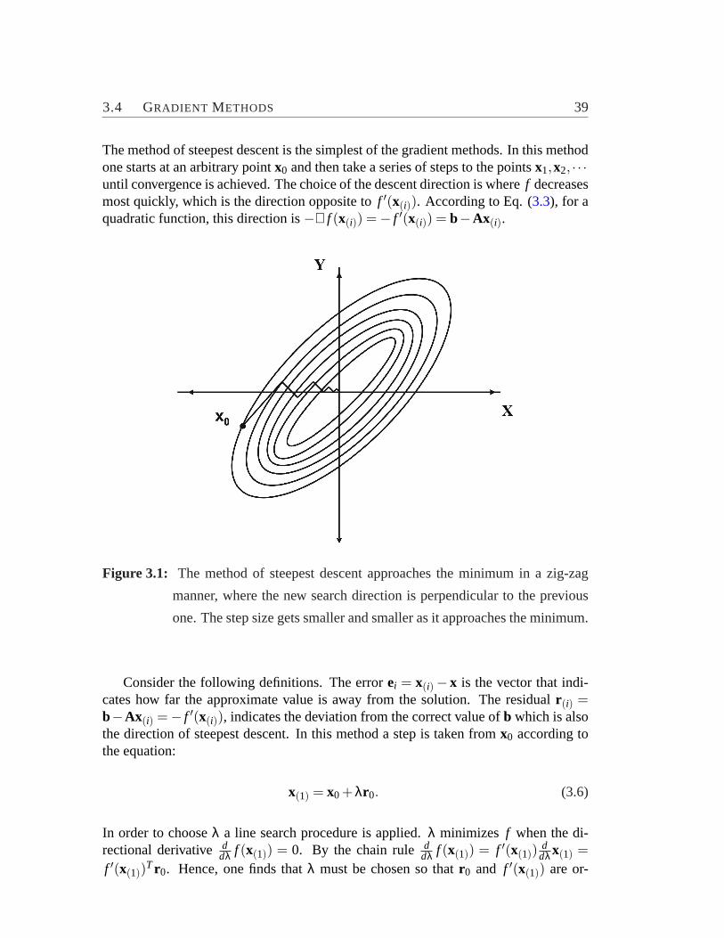
3.4 GRADIENT METHODS 39
The method of steepest descent is the simplest of the gradient methods. In this methodone starts at an arbitrary pointx0 and then take a series of steps to the pointsx1,x2, · · ·until convergence is achieved. The choice of the descent direction is wheref decreasesmost quickly, which is the direction opposite tof ′(x(i)). According to Eq. (3.3), for aquadratic function, this direction is−∇ f (x(i)) =− f ′(x(i)) = b−Ax(i).
Figure 3.1: The method of steepest descent approaches the minimum in a zig-zag
manner, where the new search direction is perpendicular to the previous
one. The step size gets smaller and smaller as it approaches the minimum.
Consider the following definitions. The errorei = x(i)− x is the vector that indi-cates how far the approximate value is away from the solution. The residualr (i) =b−Ax(i) =− f ′(x(i)), indicates the deviation from the correct value ofb which is alsothe direction of steepest descent. In this method a step is taken fromx0 according tothe equation:
x(1) = x0 +λr0. (3.6)
In order to chooseλ a line search procedure is applied.λ minimizes f when the di-rectional derivatived
dλ f (x(1)) = 0. By the chain rule ddλ f (x(1)) = f ′(x(1)) d
dλx(1) =f ′(x(1))Tr0. Hence, one finds thatλ must be chosen so thatr0 and f ′(x(1)) are or-

40 CHAPTER 3 LARGE-SCALE OPTIMIZATION
thonormal. To determineλ one considers:
− f ′(x(1))Tr0 = 0
rT(1)r0 = 0
(b−Ax(1))Tr0 = 0
(b−A(x0 +λr0))Tr0 = 0
(b−Ax0)Tr0 = λ(Ar 0)Tr0
λ =rT
0 r0
rT0 Ar 0
. (3.7)
Putting it all together the algorithm for the steepest descent is:
r (i) = b−Ax(i), (3.8)
λ(i) =rT(i)r (i)
rT(i)Ar (i)
, (3.9)
x(i+1) = x(i) +λ(i)r (i). (3.10)
Fig. 3.1 illustrates the method of steepest descent. This method is very stable, if theminimum points exist. However this method suffers from low convergence problems.For badly scaled systems, the method can end up spending an infinite number of itera-tions before locating a minimum.
3.4.2 Conjugate gradient method
As seen in the previous subsection, the reason why the method of steepest descent con-verges slowly is that it has to take a right angle turn after each step, and consequentlysearch in the same direction. The method of conjugate gradient is an attempt to mendthis problem by "learning" from experience.
Conjugacymeans that two unequal vectors,di andd j , are orthogonal with respectto any symmetric positive definite matrix,A, i.e.,
dTi .A.d j = 0. (3.11)
This can be looked upon as a generalization of orthogonality, for whichA is the unitymatrix. The idea is to let each search directionsdi be dependent on other search direc-tions searched to locate a minimum off (x) through Eq. (3.11). A set of such searchdirections are referred to asA-orthogonal, or conjugate set. It will take for a positivedefiniten-dimensional quadratic function to its minimum point in, at most,n exactlinear searches. The method is often referred to asconjugate directions.
The best way to visualize the working of conjugate directions is by comparing thespace we work in with a stretched space as shown in Fig.3.2. Fig. 3.2(a) demonstrates
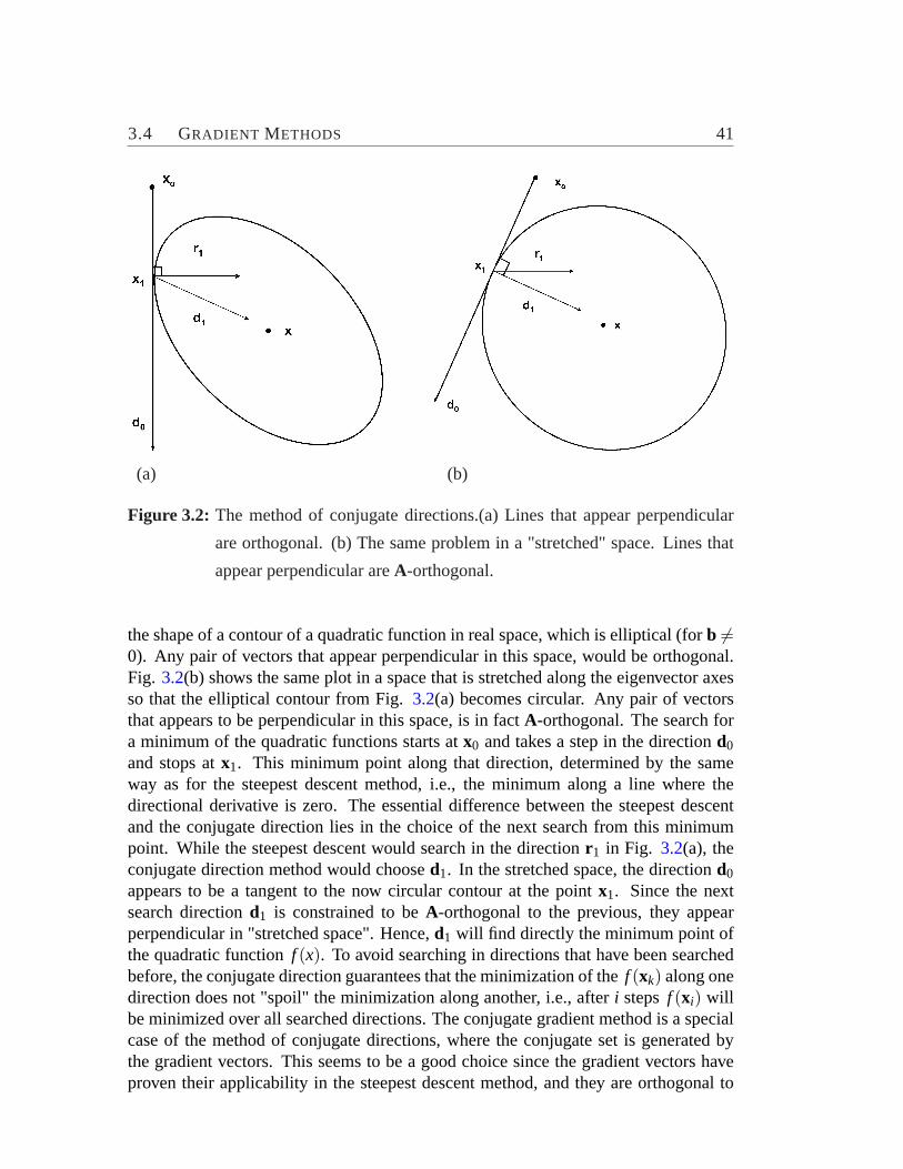
3.4 GRADIENT METHODS 41
(a) (b)
Figure 3.2: The method of conjugate directions.(a) Lines that appear perpendicular
are orthogonal. (b) The same problem in a "stretched" space. Lines that
appear perpendicular areA-orthogonal.
the shape of a contour of a quadratic function in real space, which is elliptical (forb 6=0). Any pair of vectors that appear perpendicular in this space, would be orthogonal.Fig. 3.2(b) shows the same plot in a space that is stretched along the eigenvector axesso that the elliptical contour from Fig.3.2(a) becomes circular. Any pair of vectorsthat appears to be perpendicular in this space, is in factA-orthogonal. The search fora minimum of the quadratic functions starts atx0 and takes a step in the directiond0
and stops atx1. This minimum point along that direction, determined by the sameway as for the steepest descent method, i.e., the minimum along a line where thedirectional derivative is zero. The essential difference between the steepest descentand the conjugate direction lies in the choice of the next search from this minimumpoint. While the steepest descent would search in the directionr1 in Fig. 3.2(a), theconjugate direction method would choosed1. In the stretched space, the directiond0
appears to be a tangent to the now circular contour at the pointx1. Since the nextsearch directiond1 is constrained to beA-orthogonal to the previous, they appearperpendicular in "stretched space". Hence,d1 will find directly the minimum point ofthe quadratic functionf (x). To avoid searching in directions that have been searchedbefore, the conjugate direction guarantees that the minimization of thef (xk) along onedirection does not "spoil" the minimization along another, i.e., afteri stepsf (xi) willbe minimized over all searched directions. The conjugate gradient method is a specialcase of the method of conjugate directions, where the conjugate set is generated bythe gradient vectors. This seems to be a good choice since the gradient vectors haveproven their applicability in the steepest descent method, and they are orthogonal to

42 CHAPTER 3 LARGE-SCALE OPTIMIZATION
the previous search direction. For a quadratic function, the procedure is as follows.The initial step is in the direction of the steepest descent:
d0 =− f ′(x0) =−g0, (3.12)
whereg is the gradient. Subsequently, the mutually conjugate directions are chosen sothat
dk+1 =−gk+1 +βkdk k = 0,1, · · · , (3.13)
where the coefficientβk is given by, for example, the so called Fletcher-Reeves for-mula:
βk =gT
k+1.gk+1
gTk .gk
. (3.14)
The step length along the directions is given by
λk =dT
k .gk
dTk .A.dk
, (3.15)
and the resulting iterative formula is identical to Eq. (3.2).The direct use of Eq. (3.15) will most likely not bring us to the solution inn
iterations either, the reason being the limited numerical accuracy in the computationswhich will make the search vectors lose their conjugacy. It should also be mentionedthat if the matrixA is badly scaled, the convergence will be slowed down considerably,as it was for the steepest descent method.
The conjugate gradient method is often employed to problems where the number ofvariablesn is large, and it is not unusual for the method to start generating nonsensicaland inefficient directions of search after a few iterations. For this reason it is importantto operate the method in cycles, with the first step being the steepest descent step. Oneexample of a restarting policy is to restart with steepest descent step aftern iterationsafter the preceeding restart.
3.4.3 Newton-Raphson method
The method of Newton-Raphson differs from the steepest descent and conjugate gra-dient methods in that the information of the second derivative is used to locate theminimum of a functionf (x). This results in faster convergence, but not necessarilyless computing time. The computation of the second derivatives and the handling oftheir matrix can be very time consuming, especially for large systems.
The idea behind the Newton-Raphson method is to approximate the given functionf (x) in each iteration by a quadratic function as given in Eq. (3.3) and then move to
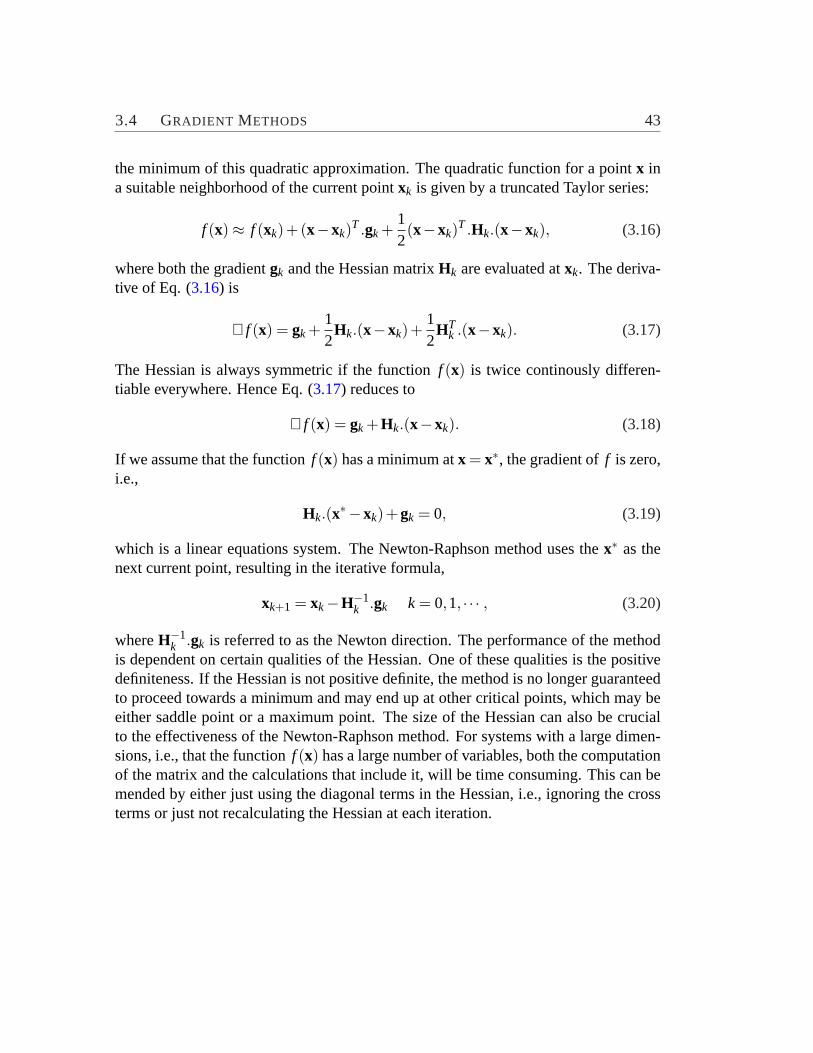
3.4 GRADIENT METHODS 43
the minimum of this quadratic approximation. The quadratic function for a pointx ina suitable neighborhood of the current pointxk is given by a truncated Taylor series:
f (x)≈ f (xk)+(x−xk)T .gk +12(x−xk)T .Hk.(x−xk), (3.16)
where both the gradientgk and the Hessian matrixHk are evaluated atxk. The deriva-tive of Eq. (3.16) is
∇ f (x) = gk +12
Hk.(x−xk)+12
HTk .(x−xk). (3.17)
The Hessian is always symmetric if the functionf (x) is twice continously differen-tiable everywhere. Hence Eq. (3.17) reduces to
∇ f (x) = gk +Hk.(x−xk). (3.18)
If we assume that the functionf (x) has a minimum atx = x∗, the gradient off is zero,i.e.,
Hk.(x∗−xk)+gk = 0, (3.19)
which is a linear equations system. The Newton-Raphson method uses thex∗ as thenext current point, resulting in the iterative formula,
xk+1 = xk−H−1k .gk k = 0,1, · · · , (3.20)
whereH−1k .gk is referred to as the Newton direction. The performance of the method
is dependent on certain qualities of the Hessian. One of these qualities is the positivedefiniteness. If the Hessian is not positive definite, the method is no longer guaranteedto proceed towards a minimum and may end up at other critical points, which may beeither saddle point or a maximum point. The size of the Hessian can also be crucialto the effectiveness of the Newton-Raphson method. For systems with a large dimen-sions, i.e., that the functionf (x) has a large number of variables, both the computationof the matrix and the calculations that include it, will be time consuming. This can bemended by either just using the diagonal terms in the Hessian, i.e., ignoring the crossterms or just not recalculating the Hessian at each iteration.

Chapter 4
Solid State Properties
There has been great burst of interest in the subject of amorphous solids, however thisarea has yet to develop any unifying principles, which can be comparable to that pro-vided by the consequence of a periodic array of atoms or ions. Many of the conceptsused in the modeling of amorphous solids are borrowed from the theory of crystallinesolids, even though they are only well understood as a consequence of lattice period-icity. In this chapter solid state properties are illustrated with some reference to thecrystals. For details refer to Refs. [1,2,86,87,88,89]
4.1 Structural Properties
4.1.1 Diffraction by crystals
Usually the structure of solids is studied through the diffraction of photons, neutronsand electrons. The diffraction depends on the structure and on the wavelength. Whenthe wavelength of the radiation is comparable with or smaller than the lattice constant,the diffracted beams are in direction quite different from the incident direction. Thefamous Bragg’s diffraction law, i.e.,2dsinθ = nλ, gives the condition for the construc-tive interference of waves scattered from the lattice points. However, in order to getdeeper understanding, one need to determine the scattering intensity from the basisatoms, i.e., the spatial distribution of the electrons.
A crystal is invariant under any translation of the formT = u1a1 + u2a2 + u3a3,whereu1,u2,u3 are integers anda1,a2,a3 are the crystal axes. The reciprocal lattice
45

46 CHAPTER 4 SOLID STATE PROPERTIES
comprises of the primitive axis vectorsb1,b2,b3, defined as
b1 = 2πa2×a3
a1.a2×a3, (4.1)
b2 = 2πa3×a1
a1.a2×a3, (4.2)
b3 = 2πa1×a2
a1.a2×a3. (4.3)
Each vector in Eq. (4.1)- Eq. (4.3) is orthogonal to two axis vectors of the crystallattice, thus
bi .a j = 2πδi j . (4.4)
A reciprocal lattice vector,G is defined as
G = ν1b1 +ν2b2 +ν3b3, (4.5)
whereν1,ν2,ν3 are integers.Any local property of a crystal is invariant underT. For example, the electron
densityn(r) is a periodic function ofr and
n(r +T) = n(r). (4.6)
The Fourier analysis of this function gives
n(r) = ∑G
nG exp(iG.r), (4.7)
and for a set of reciprocal lattice vectorsG. The Fourier coefficientsnG determine theX-ray scattering amplitude. The inversion of Eq. (4.7) gives
nG = V−1c
Zcell
dVn(r)exp(−iG.r), (4.8)
whereVc is the volume of a cell in the crystal.The set of reciprocal lattice vectorsG determines the possible X-ray reflections.
The amplitude of the electric or magnetic field vectors in the scattered electromagneticwave is given by the scattering amplitude,F defined as
F =Z
dVn(r)exp[i(k−k′).r ] =Z
dVn(r)exp(−i∆k.r), (4.9)
where
k +∆k = k′. (4.10)
4.1 STRUCTURAL PROPERTIES 47
Herek,k′ represent the wave vectors of the incident and diffracted waves, respectively.The diffraction condition is given by when the scattering vector∆k is equal to a par-ticular lattice vector, i.e.,
∆k = G. (4.11)
Hence, under the diffraction condition, the scattering amplitude for a crystal ofN cellsis given by
FG = NZ
celldVn(r)exp(−iG.r) = NSG (4.12)
Here,SG is called the structure factor and is defined over a single cell. The electronconcentrationn(r) can be considered as the superposition of electron concentrationfunctionsn j associated with each atomj of the cell. Hence, the structure factor can bewritten over all atoms of a cell as
SG = ∑j
ZdVnj(r − r j)exp(−iG.r) = ∑
jexp(−iG.r j)
ZdVnj(ς)exp(−iG.ς),
(4.13)
whereς = r − r j . The atomic form factor is defined as
f j =Z
dVnj(ς)exp(−iG.ς), (4.14)
which is integrated over all space. This factor measures the scattering power of thejthatom in the unit cell. Hence, the structure factor is given by
SG = ∑j
f j exp(−iG.r j). (4.15)
4.1.2 Investigation of structures of non-crystalline solids
In contrast to the situation with crystalline materials, the absence of periodicity meansthat the structure can no longer be reduced to considering the smallest repeat element,the unit cell. It is only possible to estimate the probability of the distribution of atomsin the vicinity of any reference atom. Diffraction methods can be used to determinethe frequency with which given interatomic distances occur in an amorphous sample.
For non-crystalline solids, in Eq. (4.12) instead of writing the structure factor ofthe basis, one can sum for all the atoms in the specimen. Further, instead of specifyingthe scattering to the reciprocal lattice vectorsG, one can consider arbitrary scatteringvectors∆k = k′−k. This is done because scattering from amorphous materials is notlimited to the reciprocal lattice vectors, which are not defined. Therefore the scatteringamplitude from an amorphous material is described by using Eq. (4.12) and Eq. (4.14)as
F(∆k) = ∑j
f j exp(−i∆k.r j). (4.16)

48 CHAPTER 4 SOLID STATE PROPERTIES
Here the summation runs over all the atoms in the material. The scattered intensity atthe scattered vector∆k is given by
I = F ∗F∗ = ∑i
∑j
fi f j exp[i∆k.(r i− r j)]. (4.17)
If α is the angle between∆k andr i− r j , then
I = ∑i
∑j
fi f j exp(iKr i j cosα), (4.18)
whereK andr i j are the magnitude of∆k andr i− r j , respectively.In an amorphous specimen the vectorr i− r j may take on all orientations and there-
fore by averaging the phase factor over a space one obtain the scattered intensity
I = ∑i
∑j
fi f jsinKr i j
Kr i j. (4.19)
For one-component system the scattered intensity is given by
I = N f2∑j
sinKr i j
Kr i j, (4.20)
where fi = f j = f for only one type of atom andN is the number of atoms. With theapproximationsr i j → 0, sinKr i j /Kr i j → 1, and with the introduction of the densityfunctionρ(r), this leads to
I = N f2[1+
Z ∞
04πr2ρ(r)
sinKrKr
dr]. (4.21)
Here,ρ(r) is the volume density of atoms at distancer from the reference atom, and4πr2ρ(r)dr is the number of atoms in a spherical shell of radiusr and thicknessdr.The functionρ(r) is thus essentially a pair correlation function and4πr2ρ(r) repre-sentsradial distribution function(RDF), g(r). This function is specially averagedone-dimensional representation of a three-dimensional structure. Introducingρ0, theaverage density of atoms in the sample investigated, the second integral in the equation
I = N f2{
1+Z ∞
04πr2[ρ(r)−ρ0]
sinKrKr
dr +Z ∞
04πr2ρ0
sinKrKr
dr}
(4.22)
can be neglected in the range of values ofK acquired in a wide-angle measurement.Amorphous solids possess no long-range order, i.e., the density functionρ(r) tends toρ0. Thus the quantity[ρ(r)− ρ0] tends to zero at distances greater than a few atomseparations and hence the first integral is dominated by the scattering mainly fromclose scattering centers. The RDF is obtain by the application of the Fourier’s integraltheorem, which eventually lead to
g(r) = 4πr2ρ(r) = 4πr2ρ0 +2rπ
Z ∞
0K
( IN f2 −1
)sin(Kr) dK. (4.23)

4.2 VIBRATIONAL PROPERTIES 49
4.2 Vibrational Properties
The vibrational properties of amorphous solids are very similar to that of the corre-sponding crystalline forms, with the exception that selection rules for transitions arerelaxed and sharp features in the density of vibrational modes are broadened due tolack of periodicity. The next sections are devoted to the discussion of vibrational ex-citations in crystals followed by anomalous properties shown by amorphous solids.This anomalous nature is more pronounced in the low temperature regime and is quiteunique to the non-crystalline phase.
4.2.1 Phonons
Figure 4.1: The Brillouin zones for a two-dimensional square lattice. The reciprocal
lattice is also a square lattice of sideb. All Bragg planes (lines, in two
dimensions) that lie within the square of side 2b centered on the origin.
These Bragg planes divide that square into regions belonging to zones 1
to 6. [Adapted from Ref. [88].]
Eq. (4.1)-Eq. (4.3) define the primitive vectors of a reciprocal lattice vectorG. Thefirst Brillouin zoneis theWigner-Seitzprimitive cell of the reciprocal lattice, i.e., the

50 CHAPTER 4 SOLID STATE PROPERTIES
set of points lying closer toK = 0 than to any other reciprocal lattice point. SinceBragg planes bisect the lines joining the origin to points of the reciprocal lattice, onecan equally well define the first zone as the set of points that can be reached from theorigin without crossing any Bragg planes. In this definition the points lying on Braggplanes are excluded, which turn out to be common to the surface of the two or morezones. Higher zones are simply other regions bounded by the Bragg planes defined asfollows:The first Brillouin zone is the set of points in reciprocal space that can be reached fromthe origin without crossing any Bragg plane. The second Brillouin zone is the set ofpoints that can be reached from the first zone by crossing only one Bragg plane. The(n+1)th Brillouin zone is the set of points not in the(n−1)th zone that can be reachedfrom thenth zone by crossing only one Bragg plane. These definitions are illustratedin Fig. 4.1 for a simple two-dimensional square lattice. These Brillouin zones areessential for the analysis of vibrational properties for crystals.
Consider elastic vibrations in a crystal. If there arep atoms in the primitive cell,there are3pbranches to the dispersion relations: 3 acoustic branches and3p−3 opticalones. The atoms vibrate against each other, but their center of mass is fixed in opticalmodes. Hence if they are ions, these motions will interact with the electric field of alight wave. However, in acoustical branches the atoms move together along with theircenter of mass.
Consider a diatomic crystal structure with massesM1, M2 connected by force con-stantC between adjacent planes. The displacements of atom of massM1 are denotedby us−1,us,us+1, · · · , and of atoms of massM2 by ϑs−1,ϑs,ϑs+1. The repeated dis-tance isa in the direction of the wave vectork. The equations of motion under theassumption that each plane interacts only with its nearest planes:
M1d2us
dt2= C(ϑs+ϑs−1−2us);
M2d2ϑs
dt2= C(us+1 +us−2ϑs). (4.24)
One can obtain a solution in the form of a traveling wave with different amplitudesu,ϑ on alternate planes:
us = uexp(iska)exp(−iωt);ϑs = ϑexp(iska)exp(−iωt). (4.25)
Eq. (4.24) and Eq. (4.25) lead to the dispersion relation:
M1M2ω4−2C(M1 +M2)ω2 +2C2(1−coska) = 0. (4.26)
For the following limiting cases the roots are:
• ka¿ 1 (very small values ofk).
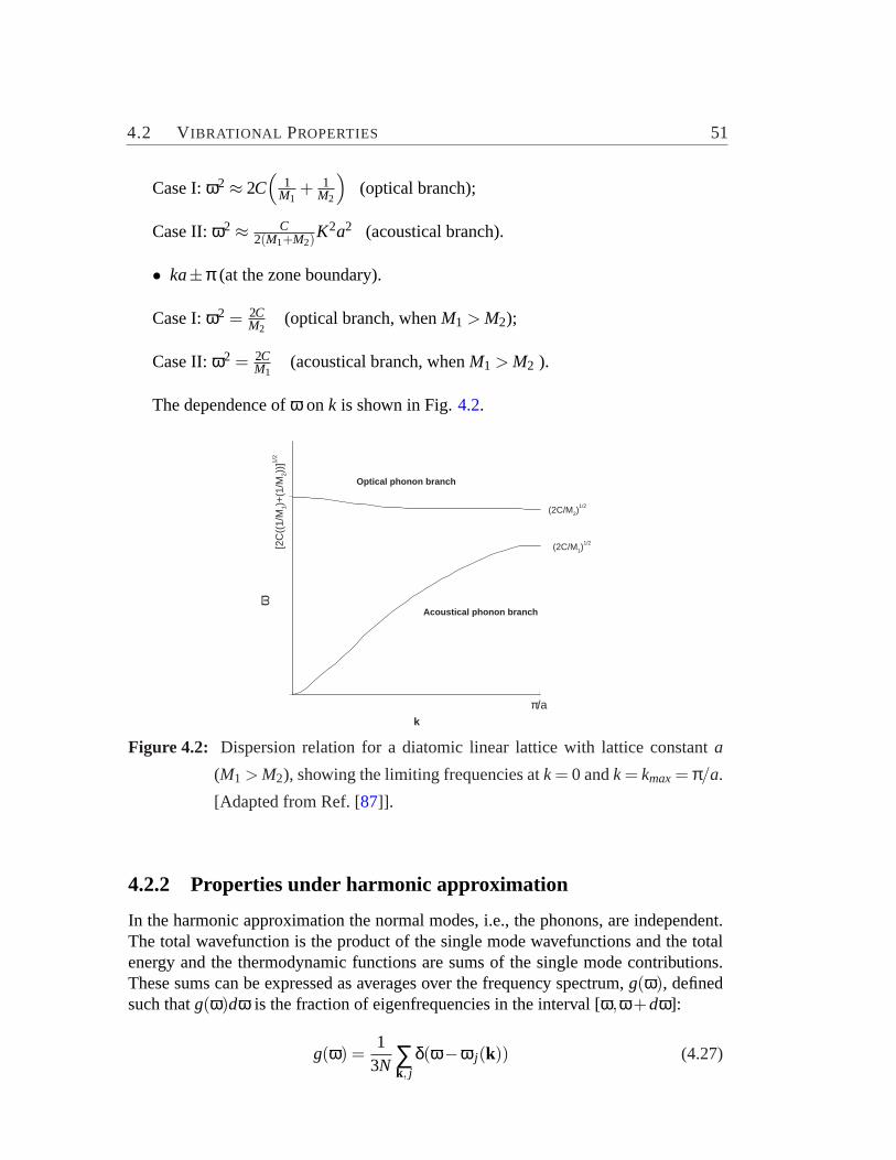
4.2 VIBRATIONAL PROPERTIES 51
Case I:ω2≈ 2C(
1M1
+ 1M2
)(optical branch);
Case II:ω2≈ C2(M1+M2)
K2a2 (acoustical branch).
• ka±π (at the zone boundary).
Case I:ω2 = 2CM2
(optical branch, whenM1 > M2);
Case II:ω2 = 2CM1
(acoustical branch, whenM1 > M2 ).
The dependence ofω onk is shown in Fig.4.2.
π/ak
[2C
((1/
M1)
+(1
/M2)
)]1/
2ω
(2C/M1)1/2
(2C/M2)1/2
Optical phonon branch
Acoustical phonon branch
Figure 4.2: Dispersion relation for a diatomic linear lattice with lattice constanta
(M1 > M2), showing the limiting frequencies atk = 0 andk = kmax= π/a.
[Adapted from Ref. [87]].
4.2.2 Properties under harmonic approximation
In the harmonic approximation the normal modes, i.e., the phonons, are independent.The total wavefunction is the product of the single mode wavefunctions and the totalenergy and the thermodynamic functions are sums of the single mode contributions.These sums can be expressed as averages over the frequency spectrum,g(ω), definedsuch thatg(ω)dω is the fraction of eigenfrequencies in the interval [ω,ω+dω]:
g(ω) =1
3N ∑k, j
δ(ω−ω j(k)) (4.27)

52 CHAPTER 4 SOLID STATE PROPERTIES
and Z ∞
0dω g(ω) = 1. (4.28)
At low frequencies the spectrum increases asω2 which is a direct consequence ofthe linear dispersion of the long wavelength acoustic modes. Usually the spectrumshows number of singularities known asvan Hove singularities, where the derivativedg(ω)/dω is discontinuous. These singularities originate from the extrema of thedispersion curves which are always present due to the periodicity.
The thermodynamic functions can be derived from the partition function
Q = tr{exp(−βH)} (4.29)
where tr stands for trace,H is the Hamiltonian andβ = 1/(kBT) with kB the Boltzmannconstant andT the absolute temperature. In the harmonic approximation the tracecan be evaluated for each mode separately, resulting in products of sums over theoccupation numbers giving
Z = Πk, jexp[−1
2β~ω j(k)]1−exp[−β~ω j(k)]
. (4.30)
The Helmholtz free energy per atom is given by:
A =− 1N
kBT lnZ =1N
kBT ∑k, j
ln{2sinh[~ω j(k)/(2kBT)]} (4.31)
= 3kBTZ
dω ln{2sinh[~ω j(k)/(2kBT)]}g(ω). (4.32)
HereN represents number of atoms. From this expression the internal energyE, thespecific heat at constant volumeCV and the vibrational entropyS per atom, can becalculated by standard thermodynamic relations:
E = A−T(∂A
∂T
)V
= 3~2
Zdωcoth[~ω/(2kBT)]ωg(ω).
(4.33)
CV =(∂E
∂T
)V
= 3kB
Zdω
( ~ω2kBT
)2{sinh2[~ω/(2kBT)]}−1g(ω).
(4.34)
S=−(∂A
∂T
)V
= 3kB
Zdω
( ~ω2kBT
coth[~ω/(2kBT)]− ln{2sinh[~ω/(2kBT)]})
g(ω).
(4.35)
At low temperatures the specific heat and entropy obey a∼T3 law, which is typicalfor an ordered lattice. In amorphous solids a leading term∼ T is found which isattributed to tunneling centers.
4.2 VIBRATIONAL PROPERTIES 53
The low temperature behavior can be approximated by the Debye spectrum. Atlow temperature the thermodynamics will be dominated by the low frequency phonons.The spectrum for low frequency is always proportional toω2, stemming from the lineardispersion for smallk. In the Debye approximation one assumes a purely quadraticbehavior ofg(ω) up to a cutoff given by,
gD(ω) =
{3
ω3D
ω2 ω≤ ωD
0 ω > ωD(4.36)
The Debye frequencyωD is often expressed in terms of a Debye temperatureΘD as
kBΘD = ~ωD. (4.37)
The Debye approximation is valid only for low temperature and the Debye frequencycan be determined from the low frequency part of the true spectrum or from the soundvelocity.
4.2.3 Anomalies in amorphous systems
Amorphous materials posses no long-range order. Their structure can be visualizedas that of a frozen-in liquid. Sound waves, the long wavelength limit of the phononsstill exist in these materials. With decreasing wavelength the sound waves will be in-creasingly scattered by the inhomogeneity on an atomic scale. This damping of thephonons by disorder is always proportional to some power ofω. When the wavelengthapproaches the atomic scale, a description of the atomic vibrations in terms of phonons(plane waves) is no longer sensible. Nevertheless there are well defined atomic vibra-tions, but with rather complicated eigenvectors (structure factors). Usually the densityof states of these vibrations are similar to their counterpart in crystals. In particular themaxima present for the crystalline form are also found in the amorphous material. Themaxima in the density of state of crystal stems from the zone boundary phonons. Thesephonons probe the short-range order which is more or less preserved in the amorphousphase. Disorder will of course broaden all features.
At low temperatures the properties of amorphous systems differ significantly fromthose of crystals [90]. Best known is the anomalous low temperature behavior of thespecific heat. In crystalsCV ∝ T3 and the proportionality constant is determined bythe sound velocities. In amorphous materials for example in glasses there are addi-tional contributions to the specific heat. BelowT ≈ 2 K the specific heat increasesapproximately linearly withT. At T ≈ 2 K there is a crossover toT5 dependence. Thelinear part in the specific heat is attributed to two-level systems, i.e., certain groups ofatoms can be envisaged as tunneling between two minimum configurations [91, 92].The anomaly in the specific heat above 2K are attributed to the localized soft harmonicvibrations [93]. A common description of the two-level systems and the soft vibra-tions was proposed in the soft potential model [94]. Refer references [94,95,97,96]
54 CHAPTER 4 SOLID STATE PROPERTIES
for details. This model assumes that, for some reaction coordinate, disorder weakensthe harmonic restoring force due to local strains. For sufficiently large local strainsthe original configuration can even become unstable, and the minimum configurationturns into a maximum. Eventually, the always present anharmonic terms stabilize theconfiguration in new minima on either side of the maximum. The maximum with twoadjoining minima forms a two-well system in the reaction coordinate. The simplestdescription of such a scenario is given by the quartic potential,
V(x) = ε[η(x/a)2 + t(x/a)3 +(x/a)4]. (4.38)
Here the scale factora is an atomic length, about half the nearest neighbor distance.For x = a and η = 1 the quadratic and quartic parts of the potential are equal. Inthis formulation of the model the energy scale factorε is equal to the value for thepotential of a single atom,εa, times the number of atoms participating in the mode,Ns. To ensure that in the two well case Eq. (4.38) represents an expansion around themaximum,η has to be restricted toη < 9
32t2. Depending on the parameters, Eq. (4.38)describes a variety of situations.
Consider first the pure symmetric case (t = 0). For η ≈ 1, V(x) is a good ap-proximation of a harmonic potential, andx describes a vibrational degree of freedom.For η < 0 we have a two-well potential with a maximum atx = 0 and minima atx = ±
√−η/2. For larger negative values ofη, when both minima are clearly de-
veloped but their distance and the barrier separating them are not too large, tunnelingtransition from one minimum to the other becomes important. In the energy schemethis corresponds to a splitting of the ground state level of one minimum into a symmet-ric and an antisymmetric state regarding both minima, i.e., one has a two-level system.The higher excited states are not important at the low temperatures considered. Foryet larger negative value ofη, i.e., increasing the separation of the minima and higherbarriers, the tunnel splitting goes to 0 and only thermally activated transitions fromone minimum to other are possible (relaxations). The asymmetry of the potential fort 6= 0 changes the boundaries of the different regimes. For example a larger value oftsuppresses the influence of the second minimum.
In this model two- and one-well model are described, causing two-level systemsand soft vibrations, respectively, by a common distribution. A fit of the potential tothe experimental data gives numbers of 20 to 80 atoms participating in the tunnelingand the soft vibrations [97, 98]. The soft vibrations occur around atoms whose localenvironment differs from the average one.
4.3 Elastic Constants
The elastic constants are of interest because of the insight they give into the nature ofthe binding forces in solids, and they are also of importance for the thermal proper-ties of solids. Polycrystalline and amorphous solids have isotropic elastic properties

4.3 ELASTIC CONSTANTS 55
and may be approximately described by fewer elastic constants than a single crystal.However the knowledge of the constants for single crystals are of fundamental signifi-cance. The elastic properties of a crystal are generally anisotropic and defined in termsof tensors.
4.3.1 Elastic strains and stresses
Consider three orthogonal axesf,g,h of unit length, embedded in an unstrained solid.After a small uniform deformation the axes distort tof′,g′,h′, such as,
f′ = (1+ εxx)f + εxyg+ εxzh;
g′ = εyxf +(1+ εyy)g+ εyzh;
h′ = εzxf + εzyg+(1+ εzz)h. (4.39)
The fractional changes of length off,g andh areεxx,εyy,εzz, respectively. The straincomponents are defined as
exx = εxx eyy = εyy ezz= εzz. (4.40)
The other non-diagonal component of the strain may be defined as the changes in theangle between the axes and considering only the linear terms as,
exy = f′.g′ ≈ εyx+ εxy;
eyz = g′.h′ ≈ εzy+ εyz;
ezx = h′.f′ ≈ εzx+ εxz. (4.41)
Using Eq. (4.40) and Eq. (4.41), Eq. (4.39) becomes
f′− f = exxf +12
exyg+12
ezxh;
g′−g =12
exyf +eyyg+12
eyzh;
h′−h =12
ezx+12
eyzg+ezzh. (4.42)
Consider a particle at the position
r = xf +yg+zh. (4.43)
After the deformation the displacement is given by
ρ = x(f′− f)+y(g′−g)+z(h′−h). (4.44)
One can write the displacement as
ρ = uf +vg+wh, (4.45)
56 CHAPTER 4 SOLID STATE PROPERTIES
where the expression for the strain components as:
exx =∂u∂x
; eyy =∂v∂y
; ezz=∂w∂z
; (4.46)
exy =∂v∂x
+∂u∂y
; eyz =∂w∂y
+∂v∂z
; ezx =∂u∂z
+∂w∂x
. (4.47)
The strain component of the typeexy as given in Eq. (4.47) can be interpreted asmade up two simple shears. In one of the shears, planes of the material normal to thex axis slide iny direction; in the other shear, planes normal toy slide inx direction
4.3.2 Stress components
The force acting on a unit area in the solid is defined as the stress. There are ninestress components:Xx,Xy,Xz,Yx,Yy,Yz,Zx,Zy,Zz. The capital letter indicates the direc-tion of the force, and the subscript indicates the normal to the plane to which the forceis applied. Thus the stress componentXx represents a force applied in thex directionto a unit area of a plane whose normal lies in thex direction. The number of inde-pendent stress components is reduced to six by applying the condition that the angularacceleration vanish, and hence that the total torque must be zero. Therefore, it followsthat
Yz = Zy; Zx = Xz; Xy = Yx;
and the independent stress components may be taken asXx,Yy,Zz,Yz,Zx,Xy.
4.3.3 Elastic compliance and stiffness constants
Hooke’s law states that for small deformations the strain is proportional to the stress.Hence, the strain components are proportional to the stress components:
exx = s11Xx +s12Yy +s13Zz+s14Yz+s15Zx +s16Xy;
eyy = s21Xx +s22Yy +s23Zz+s24Yz+s25Zx +s26Xy;
ezz= s31Xx +s32Yy +s33Zz+s34Yz+s35Zx +s36Xy;
eyz = s41Xx +s42Yy +s43Zz+s44Yz+s45Zx +s46Xy;
ezx = s51Xx +s52Yy +s53Zz+s54Yz+s55Zx +s56Xy;
exy = s61Xx +s62Yy +s63Zz+s64Yz+s65Zx +s66Xy; (4.48)
4.3 ELASTIC CONSTANTS 57
Conversely, the stress components are linear functions of the strain components:
Xx = c11exx+c12eyy+c13ezz+c14eyz+c15ezx+c16exy;
Yy = c21exx+c22eyy+c23ezz+c24eyz+c25ezx+c26exy;
Zz = c31exx+c32eyy+c33ezz+c34eyz+c35ezx+c36exy;
Yz = c41exx+c42eyy+c43ezz+c44eyz+c45ezx+c46exy;
Zx = c51exx+c52eyy+c53ezz+c54eyz+c55ezx+c56exy;
Xy = c61exx+c62eyy+c63ezz+c64eyz+c65ezx+c66exy; (4.49)
The quantitiess11,s12, · · · are called the elastic constants or elastic compliance con-stants; the quantitiesc11,c12, · · · are called the elastic stiffness constants or moduli ofelasticity. The matrix ofc’s or s’s is symmetrical, therefore thirty-six constants arereduced to twenty-one coefficients for each case. These numbers are further reduceddepending on the symmetry of the crystal.

Chapter 5
Quantum Chemical Treatment of
Solids
5.1 Overview of Quantum Chemical Methods
Quantum mechanics is the correct mathematical description of the behaviors of elec-trons and thus of chemistry. In practice, quantum mechanical equations have only beensolved exactly for one electron systems. There exist a collection of methods for ap-proximating the solution for multiple electron systems. Refer to Refs. [84,99,100,101]for details. The following sections deals with the discussion of few of the methods.
5.1.1 The Hartree-Fock method
The Hartree-Fock (HF) approximation is a starting point for more accurate methodswhich includes the effect of electron correlation. HF theory is a single determinant the-ory, where one is interested in finding a set of spin orbitalsχa such that the determinantformed from these spin orbitals,
|Ψ〉= |χ1χ2 · · ·χaχb · · ·χN〉, (5.1)
is the best possible approximation to the ground state of theN-electron system thatis described by an electronic HamiltonianHe, as given in Eq. (2.2). In the follow-ing discussions the subscript "e" is dropped as the discussion is only about electronicHamiltonian and electronic wavefunction. The non-relativisticN-electron Hamilto-nian under the Born-Oppenheimer approximation is given by
H = ∑i
h(i)+ ∑i< j
v(i, j). (5.2)
59
60 CHAPTER 5 QUANTUM CHEMICAL TREATMENT OF SOLIDS
Herehi is the one-electron term
h(i) =−12
∇2i −∑
A
ZA
r iA, (5.3)
describes the kinetic energy and the electron-nucleus Coulombic interaction ofith elec-tron. v(i, j) is a two-electron term
v(i, j) =1r i j
, (5.4)
describes the Coulomb repulsion between the electronsi and j. According to thevariational principle the "best" spin orbitals are those which minimizes the electronicenergy
E0 = 〈Ψ|H|Ψ〉= ∑a〈a|h|a〉+ 1
2∑ab
〈ab||ab〉. (5.5)
The spin orbitals are varied, constraining them only to the extent that they remainorthogonal untilE0 is minimum. This procedure leads to the HF integro-coupled-differential equation
F(i)|χi〉= εi |χi〉, (5.6)
whereεi represent the orbital energy.F is the Fock operator given by
F(i) = h(i)+∑b
Jb(i)−∑b
Kb(i). (5.7)
TheJ andK represent Coulomb and exchange operators, respectively, and are definedas
Jb(r)χa(r) =[Z
dr ′ χ∗b(r′)
1|r − r ′|χb(r ′)
]χa(r) (5.8)
Kb(r)χa(r) =[Z
dr ′ χ∗b(r′)
1|r − r ′|χa(r ′)
]χb(r) (5.9)
Eq. (5.6) can be interpreted as a set of effective one-electron Schrödinger equations forthe orbitals. They are often referred to as thecanonical Hartree-Fock equations. Thecorresponding orbitals are the canonical HF orbitals, and the eigenvalues are referredto as orbital energies.
5.1.2 Electron correlation methods
In the HF approximation, one solves equations for the behaviors of each electron inthe averaged field of the remaining(n−1)electrons. In reality, however, the electronic
5.1 OVERVIEW OF QUANTUM CHEMICAL METHODS 61
motion occur according to the actual position of other electrons. The Coulomb re-pulsion between electrons reduces sufficiently only when a correlated motion of theelectronic system takes place. This aspect of the electronic motion is absent in theHF approximation. A correlation hole is missing around every electron which pre-vent other electrons from coming too close. Consequently, the correlation energy of asystem is defined as the difference between the exact energy and the HF energy.
However, there exist several theoretical methods for treating the electron correla-tion problem. One of the formally simplest theoretical method is full configurationinteraction (FCI) method in which wavefunction is the best linear combination of allpossible configuration state functions within a given basis set. FCI is practically im-possible if there are more than a few electrons in the system. The CI wavefunction isusually truncated to singles and doubles substitution and referred as singles and dou-bles CI (CISD) method. In the following sections other methods like Second-orderMøller-Plesset perturbation theory and coupled-cluster theory are described.
5.1.2.1 Second-order Møller-Plesset Perturbation Theory
The simplest electron correlation method is Møller-Plesset perturbation theory [102],which is a special variant of Rayleigh-Schrödinger perturbation theory (RSPT). In thismethod, the Hamiltonian operator of aN-electron system is divided into two parts, anunperturbed HamiltonianH0 and a perturbationλH1
H = H0 +λH1. (5.10)
The wavefunction and energy are also expanded in a similar way and it is assumed thatthe zeroth-order wavefunctionΨ0 is an eigenfunction ofH0 with eigenvalueE0;
Ψ = Ψ0 +λΨ1 +λ2Ψ2 + · · · (5.11)
E = E0 +λE1 +λ2E2 + · · · (5.12)
By inserting Eq. (5.10)- Eq. (5.12) into Schrödinger equation and collecting terms ofthe same order inλ we get the following hierarchy of equations up to second order:
H0Ψ0 = E0Ψ0 (5.13)
(H0−E0)Ψ1 = (E1−H1)Ψ0 (5.14)
(H0−E0)Ψ2 = (E1−H1)Ψ1 +E2Ψ0. (5.15)
One can assume that the perturbed wavefunctions are orthogonal to the zeroth-orderfunction, which leads to the so-called intermediate normalization of the total wave-function〈Ψ|Ψ0〉= 1. Using this the following expressions of the energies up to secondorder is obtained:
E0 = 〈Ψ0|H0|Ψ0〉 (5.16)
E1 = 〈Ψ0|H1|Ψ0〉 (5.17)
E2 = 〈Ψ0|H1|Ψ1〉 (5.18)
62 CHAPTER 5 QUANTUM CHEMICAL TREATMENT OF SOLIDS
In the Møller-Plesset perturbation (MP2) theory the unperturbed Hamiltonian ischosen to be a sum of Fock-operators acting on the electron. Hence, the zeroth-orderenergy is the sum of the orbital energies for the occupied spin orbitals. It follows thatthe sum of the zeroth- and first-order energy equals the HF energy. In order to solvethe first-order equation, we expand the first-order wavefunction in determinantsΦµ:
Ψ1 = ∑µ
CµΦµ (5.19)
where in case of MP2 the sum runs over excited determinants with respect to theHF ground state. AllΦµ are eigenfunctions ofH0 with eigenvaluesEµ equal to thesum of the orbital energies of the spin-orbitals occupied in the given determinant. Bysubstituting Eq. (5.19) into Eq. (5.15), we get the following expression of the first-order expansion coefficients:
Cµ =−〈Φµ|H1|Ψ0〉Eµ−E0
(5.20)
The numerator contains the interaction between the configurationΦµ and the HF ref-erence function, hence, only those configurations, for which the element is non-zeroneed to be included. Singly excited configurations will not contribute due to the Bril-louin theorem. Thus, the second-order energy is given by:
E2 =−∑i> j
∑a>b
|〈Ψ0|H1|Φabi j 〉|2
ea +eb−ei−ej, (5.21)
wherei, j anda,b are occupied and virtual spin-orbitals, respectively. The applicabilityof MP2 is restricted to cases with a sufficient large HOMO-LUMO gap. If this is notthe case then the energy denominators in Eq. (5.21) become small and the perturbationexpansion diverges.
5.1.2.2 Coupled Cluster Method
The coupled cluster (CC) method has emerged in recent years as a powerful tool fortreating electron correlation to high accuracy for small- to medium-sized atoms andmolecules [103]. The advantage of this method is the size-extensivity irrespective ofthe truncation of the excitation level is employed. In CC theory the wavefunction isgenerated by an exponential excitation operator
ΨCC = exp(T)φSCF, (5.22)
where the exponential excitation operator is defined by the Taylor expansion
exp(T) = 1+ T +12!
TT +13!
TTT + · · · (5.23)
5.1 OVERVIEW OF QUANTUM CHEMICAL METHODS 63
The excitation operator may be decomposed into single, double, and possibly higherexcitation operators
T = T1 + T2 + · · · (5.24)
with
TN =( 1
N!
)2 N
∑i j ···ab···
tab···i j ··· a†
aa†b · · ·a jai . (5.25)
Here i, j, · · · anda,b, · · · refer to the occupied and unoccupied orbitals in referencedeterminant, respectively.a†
a andai refer to creation and annihilation operators. TheoperatorT is usually truncated after double excitations which defines the coupled-cluster singles and doubles (CCSD) method and wavefunction becomes [104,105].
ΨCCSD= exp(T1 + T2)φSCF. (5.26)
If we insert this wavefunction ansatz into the Schrödinger equation
(H−ECCSD)ΨCCSD= (H−ECCSD)exp(T1 + T2)φSCF = 0 (5.27)
then projecting against the reference, singly and doubly excited states, we obtain a setof equations sufficient for determining theta
i andtabi j coefficients:
〈φSCF|(H−ECCSD)(1+ T1 + T2 +12
T21 )|φSCF〉= 0
(5.28)
〈φai |(H−ECCSD)(1+ T1 + T2 +
12
T21 + T1T2 +
13!
T31 )|φSCF〉= 0
(5.29)
〈φabi j |(H−ECCSD)(1+ T1 + T2 +
12
T21 + T1T2 +
13!
T31 +
12
T22 +
14!
T41 )|φSCF〉= 0.
(5.30)
The expansion on the right-hand side terminate after the quadruple excitations sincethe Hamiltonian can couple only configurations that differ by at most two excitations.The number of equations corresponds exactly to the number of coefficients. The com-putational cost of this method rises asymptotically with the sixth power of the basis setdimension. The accuracy of the CCSD calculations can be significantly improved bysubsequently computing the effects of higher order excitations through RSPT based onFock Hamiltonian and the computed CCSD amplitude of single and double excitations.The most widely used ansatz of this type, usually denoted by CCSD(T) [106].

64 CHAPTER 5 QUANTUM CHEMICAL TREATMENT OF SOLIDS
5.1.3 Density functional theory
Density functional theory (DFT) is probably the most often used approach of compu-tational chemistry [107]. In the following the basic idea behind DFT is presented.
In the year 1964 Hohenberg and Kohn presented two fundamental theorems [108]which gave birth to modern DFT, an alternative approach to deal with many bodyproblem in electronic structure theory.
The first Hohenberg-Kohn theorem states that: The external potentialVext(r) is aunique functional of electron densityρ(r); since, in turnVext(r) fixesH we see that thefull many particle ground state is a unique functional ofρ(r). In other words: there isa unique relationship between the external potentialVext(r) (arising from the positivecharges of the nuclei) within aN electron system and its (ground state) electron densityρ(r).
Since the complete ground state energyE0 is a unique functional of the densityρ,so must be its individual parts, i.e.,
E0[ρ] = T[ρ]+Vint [ρ]+Vext[ρ]. (5.31)
This expression can be classified by parts dependent on the actual system (determinedby the external potential) and parts which are universal in the sense that the form ofthe functional is independent ofN, RA andZA.
E0[ρ] = Vext[ρ]︸ ︷︷ ︸System dependent
+ T[ρ]+Vint [ρ]︸ ︷︷ ︸System independent
(5.32)
where the system-independent part defines theHohenberg-Kohnfunctional
FHK[ρ] = T[ρ]+Vint [ρ]. (5.33)
The second Hohenberg-Kohn theorem is nothing else than the variational principleformulated for densities. Given any densityρ associated to aN electron system withthe external potentialVext, one can state that
E0≤ E[ρ] = T[ρ]+Vint [ρ]+Vext[ρ] (5.34)
with the equal sign only valid ifρ = ρ.Further the Hohenberg-Kohn functional can be identified as
FHK = T +Vee (5.35)
with potential energy term
Vee=12
Z Z ρ(r1)ρ(r2)r12
dr1dr2 +ENCL(ρ) = J(ρ)+ENCL(ρ). (5.36)

5.1 OVERVIEW OF QUANTUM CHEMICAL METHODS 65
HereJ(ρ) is the classical interaction of two charge densities andENCL(ρ) contains allthe non-classical parts. Thus, the complete energy functional can be written as
E[ρ] = T[ρ]︸︷︷︸unknown
+ J[ρ]︸︷︷︸known
+ENCL[ρ]︸ ︷︷ ︸unknown
+Z
Vextρ(r)dr︸ ︷︷ ︸
known
. (5.37)
The solution to the problem of unknown functional for kinetic energy was given byKohn and Sham [109]. They suggested to formally split this functional into two parts
T[ρ] = TS[ρ]+TC[ρ], (5.38)
whereTS[ρ] is expressed in a one particle approach similar to Hartree-Fock method,thus being well known, and the second part, still unknown part contains the differencebetween the real functionalT[ρ] and the one particle termTS[ρ], and will be treated,as well as the other, remaining parts of the total energy functional, which are stillunknown, in an approximate way. Thus one can write
E[ρ] = TS[ρ]+J[ρ]+Vext[ρ]+ENCL[ρ]+TC[ρ], (5.39)
= TS[ρ]+J[ρ]+Vext[ρ]+EXC[ρ]. (5.40)
Here theexchange-correlation functionalEXC[ρ] remains unknown and the rest arewell defined terms.TS is defined as
TS[ρ] =−12∑
i〈φi |∇2|φi〉 (5.41)
where theφi are one particle wavefunction which are determined similar to the Hartree-Fock theory, by applying the variational principle, which leads finally to theKohn-Sham equations
f KSφi = eiφi (5.42)
with theKohn-Sham operator
f KS =−12
∇2 +Z ρ(r2)
r12dr2 +VXC(r1)+∑
A
ZA
r1A. (5.43)
All that remains is the question how to derive the exchange-correlation functional.This term has to be treated on a approximative manner. There exist different func-tionals, most of them are derived from the electron density of a uniform electron gas,which can be calculated by means of statistical thermodynamics.
Local density approximation (LDA): Within the local density approximation oneassumes the density functional of aN particle system can be expressed in the form:
ELDAXC [ρ] =
Zρ(r)εXC(ρ(r))dr , (5.44)
66 CHAPTER 5 QUANTUM CHEMICAL TREATMENT OF SOLIDS
whereεXC(ρ(r)) is the exchange-correlation energy per particle of a uniform gas. Thisquantity can be further split into:
εXC(ρ(r)) = εX(ρ(r))+ εC(ρ(r)). (5.45)
The exchange part can be derived analytical as
εX(ρ(r)) =−34
(3ρ(r)π
)1/3. (5.46)
The correlation part can not be derived analytically, but can be calculated numericallywith high accuracy by means of quantum Monte Carlo simulations.
Gradient corrected functionals: Although the LDA approximation works quitewell for certain systems, one cannot expect it to perform well for those classes ofmolecules most chemists are interested in. This is mainly due to the fact that theelectron distribution within a molecule is far from being uniform. Thus the logical stepis to improve LDA is to construct functionals which depend not only on the densityρbut also on its gradient∇ρ, i.e.,
EGCXC = EGC
XC[ρ,∇ρ]. (5.47)
5.2 Ab Initio Treatment of Periodic System
Most ab initio electronic structure calculations of solids are based on DFT, with thedeficiency that no systematic improvement towards the exact result is possible. On theother hand, in the wavefunction-based methods, one improves the calculation system-atically by enlarging the basis set and by including more terms in the expansion of thewavefunction, however, at the price of a considerably higher computational cost.
A typical quantum-chemical investigation of solids, employing a wavefunctionbased approach, begins with a HF calculations and then subsequently improved byconsidering virtual excitations from the HF wavefunction in order to account for theelectron correlations. In order to solve the HF problem for the infinite periodic sys-tem, there exist mainly two kind of approaches, i.e., using Bloch and Wannier orbitals.Bloch orbitals are usually delocalized over the whole crystal lattice, whereas Wannierorbitals are localized and these are related by a unitary transformation. In the follow-ing sections these methods are described along with a discussion of another kind ofapproach based on finite cluster. Refer to Refs. [110,111] for details.
5.2.1 The finite-cluster approaches
5.2.1.1 A simple approach
This approach is well suited for the polymeric kind of system. In this approach thetotal energyEtot or correlation energyEcorr per unit cellU of a polymerU∞ can be
5.2 AB INITIO TREATMENT OF PERIODIC SYSTEM 67
obtained as the limit
E = limn→∞
E(R(Un)R′)n
, (5.48)
i.e., by performing calculations for increasing long oligomersR(Un)R′, where danglingbonds at the end of the polymer are saturated by groupsR andR′. In order to reducefinite-size effect due to end group saturation, one can consider
E = limn→∞
∆En = limn→∞
[E(R(Un+1)R′)−E(R(Un)R′)
](5.49)
i.e., the energy changes between two oligomers differing just by a single unit cell.The convergence of∆En with respect to the number of unit cells is much faster for thedynamical correlation energy than for the HF energy, due to the local character of elec-tron correlations. One can use Bloch or Wannier orbital approach for the calculationof the long-range HF energy.
5.2.1.2 Incremental approach
In the incremental approach using localized orbitals, the correlation energy per unitcell is expanded as
Ecorr = ∑i
εi + ∑i< j
∆εi j + ∑i< j<k
∆εi jk + · · · , (5.50)
where the summation overi involves localized orbitals in the reference cell, whilethose overj andk include all the localized orbitals of the crystal. The "one-body"incrementsεi = ∆εi are calculated by correlating each of the localized orbitals in turn,while others are kept frozen at the HF level. The "two-body" increments are deter-mined by considering pair of bonds and performing correlated calculations for eachchosen pair. Excitations are allowed only from the orbitals belonging to this pair, keep-ing the rest of the orbitals frozen. Hence the "two-body" increments∆εi j are definedas∆εi j = εi j − (εi + ε j), whereεi j is the correlation energy obtained by correlatingorbitals i and j. Higher-order increments are defined in an analogous way. Finally,adding all increments, with the proper weight factors determined by the occurrence inthe unit cell, one obtains the exact correlation energy per unit cell of the infinite systemas given in Eq. (5.50). The procedure described above only makes sense, if the incre-mental expansion is well convergent and can be truncated at low order increments,e.g., after second or third sum. However, the truncation of order of increments andspecial truncation for a given order is very important. In practical calculation usuallythe given order of increments is truncated including interactions up to certain nearestneighbor unit cells. The contributions from higher-order increments as well as frominteractions between more distant cells are negligible.
Localized orbitals for finite-cluster calculation: Due to the fact that electron cor-relation effects are "local", the above localized-electron picture helps to handle the
68 CHAPTER 5 QUANTUM CHEMICAL TREATMENT OF SOLIDS
problem of infinities at the correlated level. Localization of spin orbitals is readilyaccomplished by maximization of functional
L[{Φi}] = ∑i
ν2i Tiiii (5.51)
whereνi is the occupancy of the localized spin orbitalΦi and[Ti jkl ] is the localizationtensor. Various algorithms are available for the maximization ofL[{Φi}]. Followingchoices of[Ti jkl ] lead to different localization criteria:(a) Edmiston-Ruedenberg localization [112,113]:
TERi jkl = 〈Φi(1)Φk(2)|r−1
12 |Φ j(1)Φl (2)〉 (5.52)
(b) Foster-Boys localization [114,115]:
TFBi jkl =−〈Φi |r|Φ j〉 · 〈Φk|r|Φl 〉 (5.53)
(c) von Niessen localization [116]:
TNi jkl = 〈ΦiΦk|Φ jΦl 〉 (5.54)
Edmiston-Ruedenberg localization method calls for repeated transformation of two-electron integrals and is computationally expensive. Therefore Foster-Boys and vonNiessen approaches are more appropriate for large systems. All three criteria possessthe propensity of mixing ofσ andπ spin orbitals in planar molecules. This hampersthe clear interpretation of the resulting localized one-electron wavefunctions and callsfor other localization criteria, e.g., Pipek and Mezey [117], etc.
5.2.2 Bloch-orbital-based approach
During the last couple of decades, the HF and DFT problems had been solved for theinfinite periodic systems and the state of the art are present in the CRYSTAL program[118,119]. In this section the formulation of the HF theory in CRYSTAL program ispresented [120]. ConsiderΨi(r ,k) as a linear combination of Bloch functions (BF),φµ(r) (here referred as atomic orbitals, AOs):
Ψi(r ;k) = ∑µ
aµ,i(k)φµ(r ;k), (5.55)
where,
φµ(r ;k) = ∑G
ϕµ(r −Aµ−G)exp(ik ·G). (5.56)
Here,Aµ denotes the coordinate of the nucleus in the reference cell on whichϕµ iscentered, and the summation overG is extended to all set of the direct lattice vectors,G. The local functions are expressed as the linear combinations of a certain number,
5.2 AB INITIO TREATMENT OF PERIODIC SYSTEM 69
ng, of individually normalized Gaussian type functions (GTF) characterized by thesame center, with fixed coefficients,d j and exponents,α j , defined as
ϕµ(r −Aµ−G) =ng
∑j
d jg(α j ; r −Aµ−G) (5.57)
The expansion coefficients of the Bloch functions,aµ,i(k), are calculated by solvingthe Fock-matrix equation for each reciprocal lattice vector,k:
F(k)C(k) = S(k)C(k)E(k) (5.58)
in which S(k) is the overlap matrix over the BF,E(k) is the diagonal energy matrixandF(k) is the Fock matrix in the reciprocal space given by
F(k) = ∑G
FG exp(ik ·G) (5.59)
The element of the Fock matrix,FG, can be written as a sum of one-electron andtwo-electron contributions in the basis of the AO:
FG12 = HG
12+BG12. (5.60)
The one-electron contribution is the sum of the kinetic and nuclear attraction terms andare given by
HG12 = TG
12+ZG12 = 〈ϕO
1 |T|ϕG2 〉+ 〈ϕO
1 |Z|ϕG2 〉. (5.61)
The two-electron term is the sum of the Coulomb and exchange contributions:
BG12 = JG
12+KG12 = ∑
3,4∑n
Pn3,4∑
h[(ϕO
1 ϕG2 |ϕh
3ϕh+n4 )− 1
2(ϕO
1 ϕh3|ϕG
2 ϕh+n4 )]. (5.62)
ThePn density matrix elements in the AOs basis set are computed by integration overthe volume of the Brillouin zone (BZ),
Pn3,4 = 2
ZBZ
dk exp(ik ·n)∑j
a∗3, j(k)a4, j(k)θ(εF − ε j(k)), (5.63)
whereai,n denotes theith component of thenth eigenvector,θ is the step function,εF ,the Fermi energy andεn, nth eigenvalue.
5.2.3 Wannier-orbital-based approach
In Wannier-orbital-based method, instead of describing the electrons in terms of Blochorbitals, one describes them in terms of mutually orthogonal orbitals localized within
70 CHAPTER 5 QUANTUM CHEMICAL TREATMENT OF SOLIDS
the individual unit cells constituting the infinite solid. The Wannier-type orbitals arepseudo-canonical within the reference cell, i.e., they are not the most localized orbitalspossible [121]. The following discussion outline the solution of the HF problem of aninfinite periodic system in the Wannier representation.
A crystalline solid, in its ground state is composed of identical unit cells and theorbitals belonging to any other unit cell are identical to the corresponding orbitalsbelonging to any other unit cell and are related to one another by a simple translationoperation. Consider the number of orbitals in a unit cell isnc and if theα-th orbitalof a unit cell located at the position given by the vectorR j of the lattice is denoted by|α(R j)〉 then the set{|α(R j)〉;α = 1,nc; j = 1,N} denotes all the orbitals in the unitcell. The translational symmetry condition expressed in the real space can be stated as
|α(Ri +R j)〉= T(Ri)|α(R j)〉, (5.64)
whereT(Ri) is an operator which represents a translation by a vectorRi . One canwrite the total electronic energy of the solid as
E = N{
2nc
∑α=1
〈α(o)|T|α(o)〉+nc
∑α=1
〈α(o)|Z|α(o)〉
+nc
∑α,β=1
N
∑j=1
(2〈α(o)β(R j)|α(o)β(R j)〉−〈α(o)β(R j)|β(R j)α(o)〉)}
, (5.65)
where|α(o)〉 denotes an orbital centered in the reference unit cell. By assuming trans-lation invariance in real space, the total HF energy of the infinite solid is expressedin terms of a finite number of orbitals. In order to make energy given in Eq. (5.65)stationary with respect to the first-order variations in the orbitals, subjected to the or-thogonality constraint, HF operator is obtained and defined as
F = T +Z+2∑β
Jβ−∑β
Kβ. (5.66)
The conventional Coulomb and exchange terms are defined as
Jβ|α〉= ∑j〈β(R j)| 1
r12|β(R j)〉|α〉, (5.67)
and
Kβ|α〉= ∑j〈β(R j)| 1
r12|α〉|β(R j)〉, (5.68)
respectively. In order to impose the requirement of obtaining localized Wannier or-bitals, a projector operators corresponding to the orbitals centered in the unit cells in asufficiently large neighborhood of the reference cell is introduced and given by
(T +Z+2J−K + ∑k∈N
∑γ
λkγ|γ(Rk)〉〈γ(Rk)|α〉= εα|α〉. (5.69)
5.2 AB INITIO TREATMENT OF PERIODIC SYSTEM 71
Here |α〉 stands for|α(o)〉, an orbital centered in the reference cell,N collectivelydenotes the unit cells in the neighborhood. The choice ofN will dictate the systemunder consideration. The more delocalized electrons of the system are, the largershould be theN. The shift parametersλk
γ are the shift parameters associated withthe corresponding orbital ofN. For perfect orthogonality and localization, their valuesshould be infinitely high. Here the projection operator along with the shift parameterssimply pays a role of a localizing potential, since upon convergence their contributionto the HF equation vanishes. The orbitals contained in unit cell located farther thanthose inN should be automatically orthogonal to the reference cell orbitals. It is easyto see that the orthogonality of the neighboring orbitals to the reference cell orbitalsalong with translation symmetry of the infinite solid makes these orbitals as Wannierfunctions.


Part II
Applications
73

Chapter 6
Structural Properties
A variety of experimental techniques, particularly diffraction experiments can pro-vide information concerning microscopic structure of amorphous solids. However,this information is limited almost entirely to the first two coordination shells, i.e., thebond lengths and angles of nearest-neighbor atoms comprising the basic structural unit.Even for monoatomic systems the RDF derived from scattering experiments have thedifficulty, that peaks other than the first and second cannot be uniquely associated witha particular interatomic correlation. These are made up from a variety of contributionsfrom higher-lying shells. This matter gets more complicated for multicomponent sys-tems. One solution to these difficulties is the construction of models using theoreticalmethods like MD and MC.
In the following sections the discussion of structural properties of amorphous formsderived from ZSM-5 is presented, which were obtained using MD simulations.
6.1 Computational Details
The calculations were carried out with a modified and extended version [122] of thecode of Oligschleger and Laird [123].
6.1.1 Interaction potential
The pairwise atomic interaction potential proposed by Krameret al. [124] was used inall simulations. It was parameterized using data fromab initio calculations and exper-iment for achieving high accuracy and transferability. This potential has already beensuccessfully applied for modelling of crystalline zeolite systems [125]. The functionalform is a combination of Buckingham and Coulomb type and is given by
φ(rαβ) =qαqβe2
rαβ+Aαβ exp(−Bαβrαβ)−
Cαβ
r6αβ
. (6.1)
75
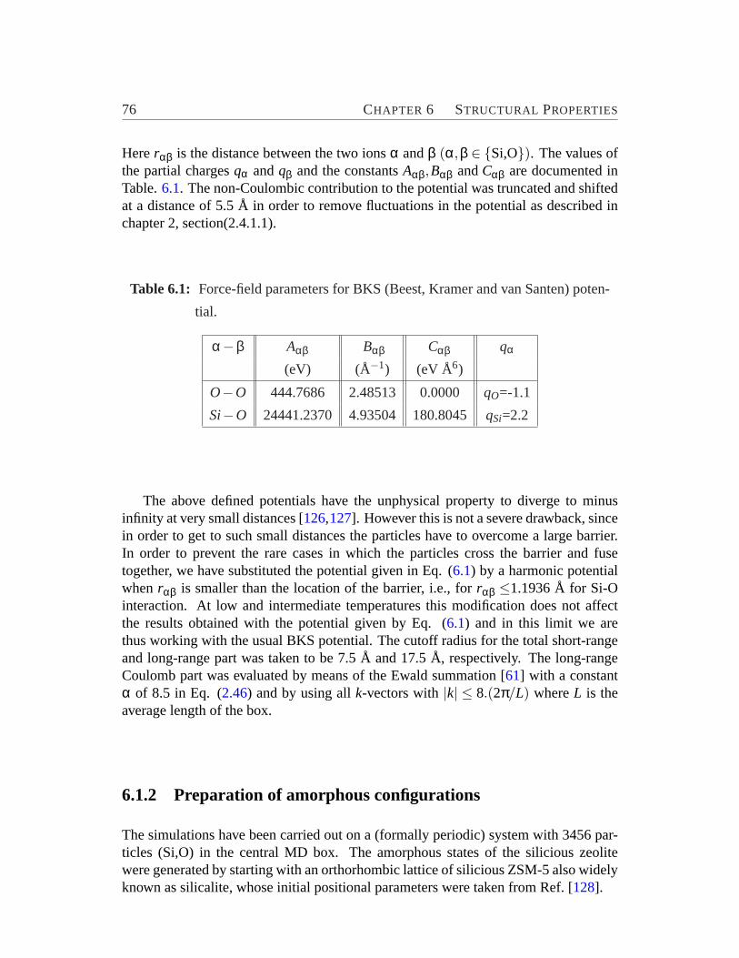
76 CHAPTER 6 STRUCTURAL PROPERTIES
Hererαβ is the distance between the two ionsα andβ (α,β ∈ {Si,O}). The values ofthe partial chargesqα andqβ and the constantsAαβ,Bαβ andCαβ are documented inTable.6.1. The non-Coulombic contribution to the potential was truncated and shiftedat a distance of 5.5 Å in order to remove fluctuations in the potential as described inchapter 2, section(2.4.1.1).
Table 6.1: Force-field parameters for BKS (Beest, Kramer and van Santen) poten-
tial.
α−β Aαβ Bαβ Cαβ qα
(eV) (Å−1) (eV Å6)
O−O 444.7686 2.48513 0.0000 qO=-1.1
Si−O 24441.2370 4.93504 180.8045 qSi=2.2
The above defined potentials have the unphysical property to diverge to minusinfinity at very small distances [126,127]. However this is not a severe drawback, sincein order to get to such small distances the particles have to overcome a large barrier.In order to prevent the rare cases in which the particles cross the barrier and fusetogether, we have substituted the potential given in Eq. (6.1) by a harmonic potentialwhenrαβ is smaller than the location of the barrier, i.e., forrαβ ≤1.1936 Å for Si-Ointeraction. At low and intermediate temperatures this modification does not affectthe results obtained with the potential given by Eq. (6.1) and in this limit we arethus working with the usual BKS potential. The cutoff radius for the total short-rangeand long-range part was taken to be 7.5 Å and 17.5 Å, respectively. The long-rangeCoulomb part was evaluated by means of the Ewald summation [61] with a constantα of 8.5 in Eq. (2.46) and by using allk-vectors with|k| ≤ 8.(2π/L) whereL is theaverage length of the box.
6.1.2 Preparation of amorphous configurations
The simulations have been carried out on a (formally periodic) system with 3456 par-ticles (Si,O) in the central MD box. The amorphous states of the silicious zeolitewere generated by starting with an orthorhombic lattice of silicious ZSM-5 also widelyknown as silicalite, whose initial positional parameters were taken from Ref. [128].
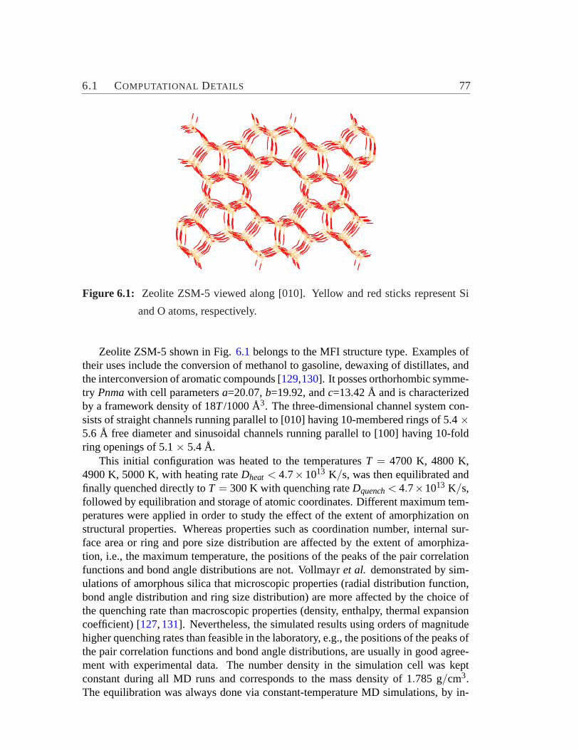
6.1 COMPUTATIONAL DETAILS 77
Figure 6.1: Zeolite ZSM-5 viewed along [010]. Yellow and red sticks represent Si
and O atoms, respectively.
Zeolite ZSM-5 shown in Fig.6.1belongs to the MFI structure type. Examples oftheir uses include the conversion of methanol to gasoline, dewaxing of distillates, andthe interconversion of aromatic compounds [129,130]. It posses orthorhombic symme-try Pnmawith cell parametersa=20.07,b=19.92, andc=13.42 Å and is characterizedby a framework density of 18T/1000 Å3. The three-dimensional channel system con-sists of straight channels running parallel to [010] having 10-membered rings of 5.4×5.6 Å free diameter and sinusoidal channels running parallel to [100] having 10-foldring openings of 5.1× 5.4 Å.
This initial configuration was heated to the temperaturesT = 4700 K, 4800 K,4900 K, 5000 K, with heating rateDheat < 4.7×10¹³ K/s, was then equilibrated andfinally quenched directly toT = 300 K with quenching rateDquench< 4.7×10¹³ K/s,followed by equilibration and storage of atomic coordinates. Different maximum tem-peratures were applied in order to study the effect of the extent of amorphization onstructural properties. Whereas properties such as coordination number, internal sur-face area or ring and pore size distribution are affected by the extent of amorphiza-tion, i.e., the maximum temperature, the positions of the peaks of the pair correlationfunctions and bond angle distributions are not. Vollmayret al. demonstrated by sim-ulations of amorphous silica that microscopic properties (radial distribution function,bond angle distribution and ring size distribution) are more affected by the choice ofthe quenching rate than macroscopic properties (density, enthalpy, thermal expansioncoefficient) [127,131]. Nevertheless, the simulated results using orders of magnitudehigher quenching rates than feasible in the laboratory, e.g., the positions of the peaks ofthe pair correlation functions and bond angle distributions, are usually in good agree-ment with experimental data. The number density in the simulation cell was keptconstant during all MD runs and corresponds to the mass density of1.785 g/cm3.The equilibration was always done via constant-temperature MD simulations, by in-
78 CHAPTER 6 STRUCTURAL PROPERTIES
tegrating the equation of motion with the velocity form of the Verlet algorithm usingperiodic boundary conditions. The equilibration time was about 0.6 ns correspondingto 3× 10⁵ integration steps. The time step was kept sufficiently small to guaranteea negligible drift of the total energy. We used the velocity rescaling method, wherewe averagedT(ti) over a period of 20 time steps[Tav = 1
20 ∑m+19i=m T(ti)] and scaled the
velocities after each period by√
T0/Tav with T0 being the "desired" temperature andTav being the averaged temperature.
We monitor the atomic displacements during the course of MD runs by
∆R(t) =√
∑n
[Rn(t)−Rn(0)]2 (6.2)
whereRn(t) is the position vector of particlen at timet andRn(0) is the one at thestarting or reference configuration. If the total displacement of the atoms exceeds acutoff value, and the residence time of the atoms in the new positions also exceeds aminimal period of at least three times the period of a typical soft vibrational mode, thenew positions of the particles were accepted as a starting point for the determinationof a possible new minimum configuration. The cutoffs of displacements and residenttime are chosen to avoid spurious minima. All stored coordinates were then quenchedto T = 0K using a combined steepest-descent-conjugate-gradient (SDCG) algorithm[132] to locate the nearest minimum configuration. These were further used for theanalysis of the structural properties of the amorphous material.
6.2 Short-Range Order
To get insight into two-body structural correlation we have calculated total and partialpair-distribution functions from the MD trajectories. Partial pair-distribution functionsgαβ are calculated from
〈nαβ(r)〉∆r = 4πr2∆rρNcβgαβ(r) (6.3)
wherenαβ∆r is the number of particles of speciesβ in a shell of thickness∆r, and ra-diusr around a particle of speciesα and〈. . .〉 represents the ensemble average and av-erage over all particles of speciesα. ρN is the total number density(N/V,N = Nα +Nβ)andcβ is the concentration of speciesβ. The contributions to the total pair-distributionfunction can be assigned by the peaks obtained in the partial pair-distribution functions.The computed total pair-distribution function and partial pair-distribution functions ofSi-O, O-O and Si-Si are shown in Fig.6.2. The most intense peak in the total pair-distribution function (Fig. 6.2(a)) arises fromgSi−O (Fig. 6.2(b)), smaller peaks atlarger distances fromgO−O (Fig. 6.2(c)) andgSi−Si (Fig. 6.2(d)). From the positionsof these peaks we conclude that the Si-O bond length is 1.62± 0.04 Å and the nearestneighbor O-O and Si-Si distances are 2.61± 0.21 Å and 3.19± 0.15 Å , respectively.
6.3 CONNECTIVITY OF THE ELEMENTARY UNITS 79
The errors are obtained from the full width at half maximum (FWHM). The physi-cal significance of the small peaks observed at smallerr than the most intense peaksappearing in Figs.6.2(c) and6.2(d) are discussed later.
The average coordination number (CN) of speciesα surrounded by speciesβ, Zαβ,is one of the most important pieces of information that can be obtained by performingintegration around the first peak in the pair-distribution function.
Zαβ(R) = 4πρβ
Z R
0gαβ(r)r
2dr, (6.4)
Here R is the cutoff radius, usually chosen as the position of the minimum after themost intense peak ofgαβ(r). For this integration the cutoff radii for Si-O, O-O andSi-Si are taken as 1.8 Å , 3.1 Å and 3.4 Å, respectively. From this analysis it is foundthat Si atoms are on the average coordinated by 3.99 O atoms and surrounded by3.95 Si atoms. Similarly O atoms are coordinated by 2.00 Si atoms and surrounded by6.02 O atoms. These findings indicate that the most common structural feature are allcorner-sharing SiO4 tetrahedra. The deviations from this pattern are discussed below.
The three-body correlations in amorphous ZSM-5 based material are examined andcompared to the crystalline ZSM-5 through bond angle distributions plotted in Fig.6.3,which give further information on local structural units. The O-Si-O angle distributionhas the main peak at108◦ with FWHM of 12.6◦. The O-O-O angle distribution has anintense sharp peak at59.4◦ with FWHM of 7.2◦ and the O-O-Si angle distribution hasa main peak at35.1◦ with FWHM of 6.2◦. These peaks arise from atoms belongingto the same SiO4 tetrahedra. For an ideal tetrahedron the O-Si-O, O-O-O and O-O-Siangles are109.47◦, 60◦ and35.26◦, respectively. The small deviations from the idealvalues show that slightly distorted SiO4 tetrahedra are the basic structural unit. Besidesthese peaks other intense peaks related to the connectivity between the SiO4 tetrahedraare present. Similar to the pair-distribution functions in Fig.6.2 smaller peaks atunexpected positions are observed in Fig.6.3. All these features will be analyzed inthe next section.
6.3 Connectivity of the Elementary Units
Considering the peaks of the pair-distribution and bond angle distribution functionswe can interprete that the SiO4 tetrahedra are linked in two ways as shown in Fig.6.4.The model shown in Fig.6.4(a), corresponds to the usual corner-sharing tetrahedranetwork. This structural pattern can be inferred from the peak of the Si-O-Si angledistribution at157◦ with a broad FWHM of40◦, which represents the connectivity be-tween two Si atoms present in neighboring tetrahedra with corner-sharing. The broadSi-O-Si angle distribution in the amorphous phase compared to the one obtained inthe crystal indicates a considerable amount of flexibility in the Si-O-Si angle which isa major source of the disorder and allows for relaxation in a strained system. It has

80 CHAPTER 6 STRUCTURAL PROPERTIES
even been shown by ball milling experiments of Kosanovicet al. [19] that breakingof these Si-O-Si bonds occurs in high silica zeolites and results in the collapse of thecrystal structure leading to the formation of the amorphous phase. In the Si-Si-O an-gle distribution the peak around21◦ comes from two silicon atoms bound to the sameoxygen. The broad distribution from80◦ to 180◦ in the O-O-O angle stems from Oatoms bound to different Si atoms. The bond angle distribution for Si-Si-Si is peakedat59◦ stemming mainly from Si atoms at their nearest neighbor distance of≈ 3 Å, andexhibits a broad maximum at106◦, hinting to a pattern in which Si is distorted tetra-hedrally surrounded by four Si atoms at≈ 5 Å. The first peak points to the existenceof 3-fold rings in this ZSM-5 based amorphous form, whereas the broad maximumresults from the usual coordination between SiO4 tetrahedra also present in the crystal.
The positions of the first and less intense peaks ing0−0 andgSi−Si occurring around2.2 Å and 2.5 Å , respectively, look surprising at first glance. But selectively collect-ing the coordinates of such configurations provides strong evidence for the presenceof edge-sharing SiO4 tetrahedra. These are present in small percentage of around1%-4% (depending on the extent of amorphization) in the ensemble of collected con-figurations. This model of edge-sharing between tetrahedra as shown in Fig.6.4(b),is also in agreement with small peaks appearing in the bond angle distributions ofO-Si-O at83◦, Si-O-Si at95◦, O-O-Si at48◦ and Si-Si-O at42◦. These are relatedto four atoms, i.e., the Si centers of two edge-shared tetrahedra as well as the bridg-ing O atoms. The peak at83◦ in the O-Si-O bond angle distribution shows that theedge-shared tetrahedra are distorted severely. Edge sharing tetrahedra are also foundin nature in the SiO2 allotrope W-silica [133] and the silicate mineral leucophoeniciteMn7(SiO4)3(OH)2 [134]. We note that in Car-Parrinello molecular dynamics studiesof dehydroxylated silica surface also edge-shared tetrahedra are observed [135]. How-ever, the edge-shared tetrahedral structures in nature are quite rare, which is usuallyexplained by Pauling’s third rule in terms of Coulombic repulsion between the cationssharing polyhedral units. Pauling’s third rule states that the presence of shared edgesand especially of shared faces in a coordinated structure decreases its stability. Viola-tion of the rule is strong evidence that the structure is covalent.
In the past molecular orbital studies at the SCF-Xα and CNDO/2 level on the rhom-bohedral molecule Si2O2 and two silicate tetrahedra sharing a common edge and sat-urated with hydrogens at the periphery, i.e., Si2O6H4, have shown that covalent forcesplay an important role in causing edge-sharing type distortions [136,137]. In order toanalyze the validity of the results for such structural units obtained via MD, we carriedout geometry optimizations using gradient-corrected DFT, HF and MP2 calculationson the edge-shared model system Si2O6H4. The DFT and MP2 calculations were per-formed using the TURBOMOLE [138] and MOLPRO [139,140] program packages,respectively. Geometric parameters for the bridged unit for edge-shared tetrahedraare presented in Table6.2. It is obvious that the result of MD for the amorphousform derived from ZSM-5 is consistent with the experimental data for W-silica and thequantum chemical values for the edge-sharing model system. Note that the DFT andMP2 calculations on the model system do not include the effect of the surroundings.
6.3 CONNECTIVITY OF THE ELEMENTARY UNITS 81
We have also carried out solid-stateab initio calculations of the edge-sharing system,which include the effect of a condensed environment. The details of these calculationsare presented in Chapter 8.
Frequency calculations at the HF-level on the edge-shared model system give allpositive frequencies indicating that the structure corresponds to a local minimum. Inthe polarized Raman spectra of vitreous SiO2, theD1 defect line at 495cm−1 was leftunassigned [141,157]. We suggest that this could be due to the out-of-plane bendingmotion of the bridged unit, which was obtained in our frequency calculation on theedge-shared model system at 510cm−1. It is fair to note, however, that other inter-pretations also exist, i.e., no edge-sharing tetrahedra were observed in Car-Parrinellodynamics of vitreous silica and theD1 defect line was associated with a breathingmotion of 3-fold rings [142].
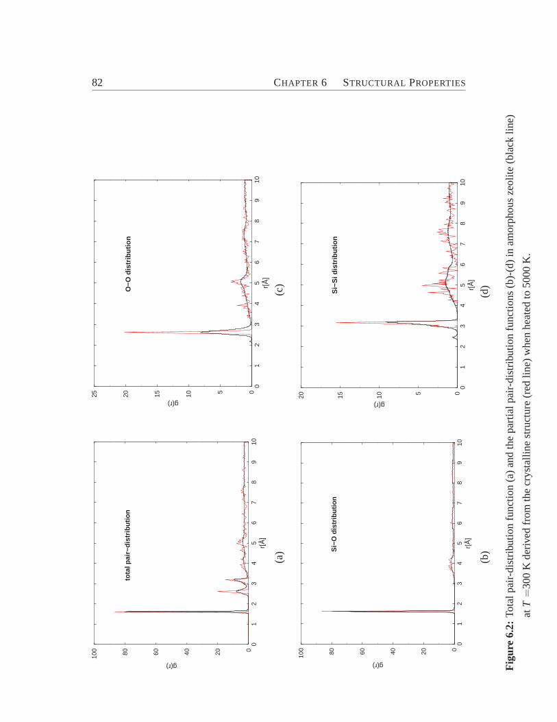
82 CHAPTER 6 STRUCTURAL PROPERTIES
01
23
45
67
89
10r[
Å]
020406080100
g(r)
tota
l pai
r−d
istr
ibu
tio
n
01
23
45
67
89
10r[
Å]
0510152025
g(r)
O−O
dis
trib
uti
on
(a)
(c)
01
23
45
67
89
10r[
Å]
020406080100
g(r)
Si−
O d
istr
ibu
tio
n
01
23
45
67
89
10r[
Å]
05101520
g(r)
Si−
Si d
istr
ibu
tio
n
(b)
(d)
Fig
ure
6.2:
Tota
lpai
r-di
strib
utio
nfu
nctio
n(a
)an
dth
epa
rtia
lpai
r-di
strib
utio
nfu
nctio
ns(b
)-(d
)in
amor
phou
sze
olite
(bla
cklin
e)
atT
=30
0K
deriv
edfr
omth
ecr
ysta
lline
stru
ctur
e(r
edlin
e)w
hen
heat
edto
5000
K.
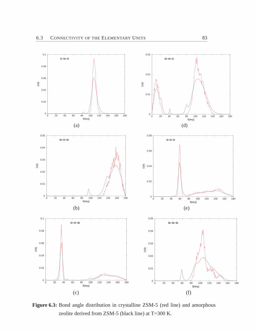
6.3 CONNECTIVITY OF THE ELEMENTARY UNITS 83
0 20 40 60 80 100 120 140 160 180θ[deg]
0
0.02
0.04
0.06
0.08
0.1
D(θ
)
O−Si−O
0 20 40 60 80 100 120 140 160 180θ[deg]
0
0.01
0.02
0.03
D(θ
)
Si−Si−O
(a) (d)
0 20 40 60 80 100 120 140 160 180θ[deg]
0
0.01
0.02
0.03
0.04
0.05
D(θ
)
Si−O−Si
0 20 40 60 80 100 120 140 160 180θ[deg]
0
0.02
0.04
0.06
0.08
D(θ
)
O−O−O
(b) (e)
0 20 40 60 80 100 120 140 160 180θ[deg]
0
0.02
0.04
0.06
0.08
0.1
D(θ
)
O−O−Si
0 20 40 60 80 100 120 140 160 180θ[deg]
0
0.01
0.02
0.03
0.04
0.05
D(θ
)
Si−Si−Si
(c) (f)
Figure 6.3: Bond angle distribution in crystalline ZSM-5 (red line) and amorphous
zeolite derived from ZSM-5 (black line) at T=300 K.
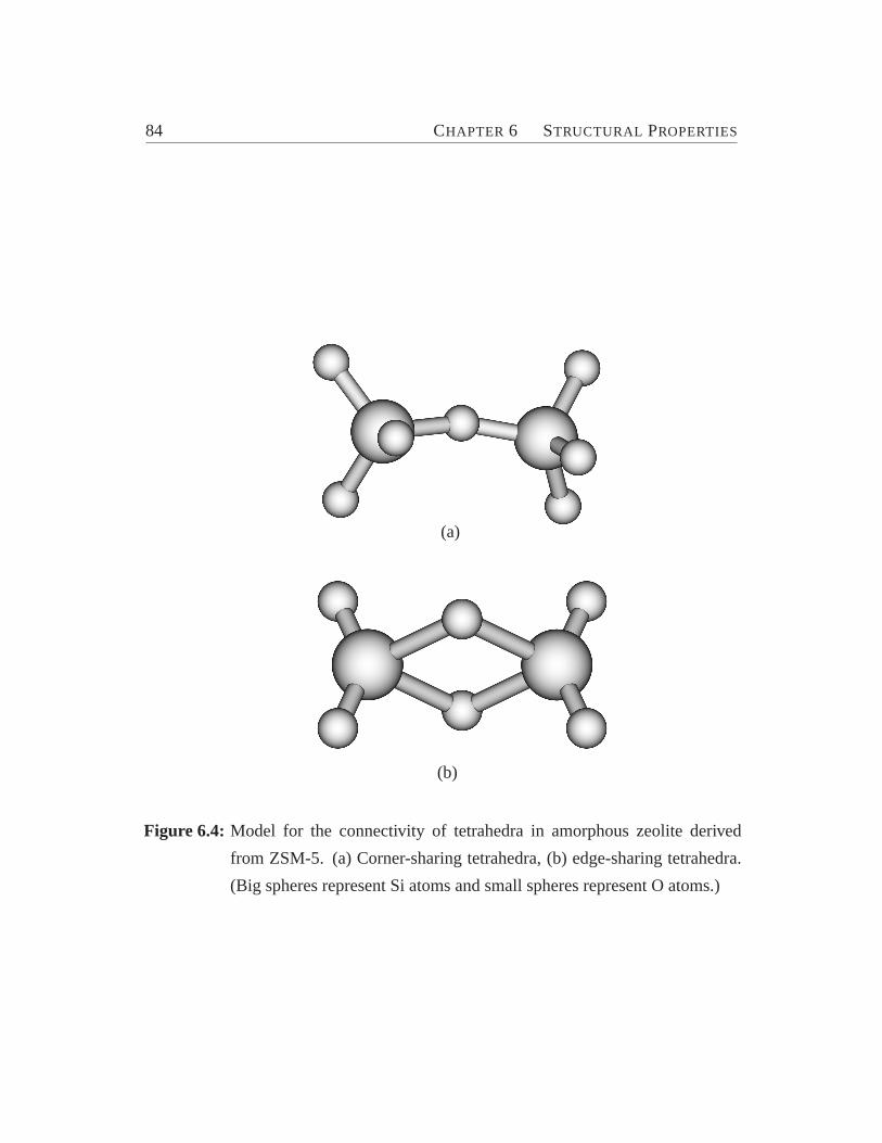
84 CHAPTER 6 STRUCTURAL PROPERTIES
(a)
(b)
Figure 6.4: Model for the connectivity of tetrahedra in amorphous zeolite derived
from ZSM-5. (a) Corner-sharing tetrahedra, (b) edge-sharing tetrahedra.
(Big spheres represent Si atoms and small spheres represent O atoms.)
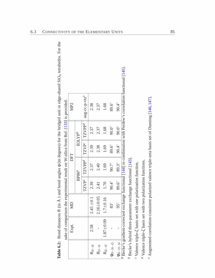
6.3 CONNECTIVITY OF THE ELEMENTARY UNITS 85
Tabl
e6.
2:B
ond
dist
ance
sR
(inÅ
)an
dbo
ndan
glesφ
(inde
gree
s)fo
rth
ebr
idge
dun
itin
edge
-sha
red
SiO
4te
trah
edra
.F
orth
e
sake
ofco
mpa
rison
the
expe
rimen
talr
esul
ton
W-s
ilica
from
Ref
.[13
3]is
prov
ided
.
Exp
t.M
DD
FT
MP
2
BP
86a
B3L
YP
b
TZ
VP
cT
ZV
PPd
TZ
VP
cT
ZV
PPd
aug-
cc-p
-vtze
RS
i−S
i2.
582.
45±0
.12.
392.
372.
392.
372.
38
RO−O
-2.
16±0
.05
2.41
2.40
2.38
2.37
2.37
RS
i−O
1.87±0
.09
1.7±
0.16
1.70
1.69
1.69
1.68
1.68
φ O−S
i−O
-83◦
90.4◦
90.7◦
89.6◦
90.0◦
89.6◦
φ Si−
O−S
i-
95◦
89.6◦
89.3◦
90.4◦
90.0◦
90.4◦
aB
ecke
’sgr
adie
nt-c
orre
cted
exch
ange
func
tiona
l[14
4]in
com
bina
tion
with
Per
dew
’sco
rrel
atio
nfu
nctio
nal[14
5].
bB
ecke
’shy
brid
thre
e-pa
ram
eter
exch
ange
func
tiona
l[14
3].
cVa
lenc
etr
iple
-ζba
sis
setw
ithon
epo
lariz
atio
nfu
nctio
n.d
Vale
nce
trip
le-ζ
basi
sse
twith
two
pola
rizat
ion
func
tions
.e
Aug
men
ted
corr
elat
ion-
cons
iste
ntpo
lariz
edva
lenc
etr
iple
-zet
aba
sis
seto
fDun
ning
[14
6,14
7].
86 CHAPTER 6 STRUCTURAL PROPERTIES
6.4 Extent of Amorphization
It was shown recently that there is a direct connection between the percentage of crys-tallinity of partially crystalline zeolitic material and its catalytic properties and ionexchange capacity [24,28,148]. If such chemical properties are based mainly on elec-tronic effects, accurate quantum chemical calculations are needed for their investiga-tion and explanation. However, in zeolitic systems steric effects play a great role todirect selectivities of reactions. These can be investigated by analysis of structures ob-tained by MD. Hence we choose a semiquantitative description to analyze the extentof amorphization, which is similar to the percentage of XRD crystallinity advocatedby Nicolaides as in Eq. (1.1) [28]. In order to get a measure independent from thenumber of atoms in the central MD box we choose the energy per atom as a criterionto describe the extent of amorphization of the system. We define the "percentage ofenergy crystallinity" (PEC), i.e.,
PEC=Eamorphous−Econ f iguration
Eamorphous−Ecrystalline×100 (6.5)
as a normalized dimensionless measure of the extent of amorphization. HereEamorphous
corresponds to the energy per atom of the maximum amorphized structure we haveobtained after minimization in our simulation, i.e., -16.90 eV/atom (in the part of con-figurational space spanned in our simulation no higher lying minimum occurs), andEcrystalline corresponds to the energy per atom of the crystalline ZSM-5 system, i.e.,-17.17 eV/atom.Econ f igurationstands for the energy of the structure whose PEC we areinterested in. It should be mentioned that clearly our definition of PEC depends on themaximum extent of amorphization obtained in the simulations, i.e., on the maximumtemperature (here 5000 K) as well as the quenching rate (here 4.7× 10¹² K/s).
As shown in Fig. 6.5, the comparison between the cross section of crystallineZSM-5 and the simulated ZSM-5 based amorphous structure with different extent ofamorphization, the amorphization leads to local disorder and partial collapse of theframework structure. It is mainly this modification of pores and cavities which mayallow a tuning of properties of significant interest.
6.4.1 Defect in coordination number
In Fig. 6.6 the distribution of coordination numbers (Z) for O atoms (ZO) and Siatoms (ZSi) for different PEC is given. If the interatomic distancer < 1.8 Å (i.e., thedistances corresponding to the first peak in the pair-distribution function Fig.6.2 (a))then the atoms are considered to be neighbors. One can easily observe the fraction ofcoordination defects, i.e., atoms with coordination numbers other than the ideal ones(ZO=2 andZSi=4) decrease with PEC. Even in highly amorphized structures (low PEC)95% of O atoms and 90% of Si atoms remain 2- and 4-coordinated, respectively.
Only 3% of the O atoms are under-coordinated (ZO=1) and 2% over-coordinated(ZO=3). In the case of the Si atoms around 9% are under-coordinated (ZSi=3) and
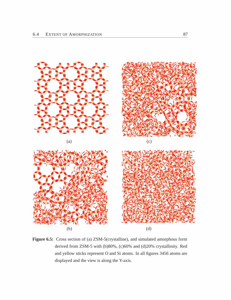
6.4 EXTENT OF AMORPHIZATION 87
(a) (c)
(b) (d)
Figure 6.5: Cross section of (a) ZSM-5(crystalline), and simulated amorphous form
derived from ZSM-5 with (b)80%, (c)60% and (d)20% crystallinity. Red
and yellow sticks represent O and Si atoms. In all figures 3456 atoms are
displayed and the view is along the Y-axis.

88 CHAPTER 6 STRUCTURAL PROPERTIES
0 10 20 30 40 50 60 70 80 90 100PEC
0.85
0.9
0.95
1
Dis
trib
utio
n of
Coo
rdin
atio
n N
umbe
r
ZSi=4ZO=2
(a)
0 10 20 30 40 50 60 70 80 90 100PEC
0
0.02
0.04
0.06
0.08
0.1
0.12
Dis
trib
utio
n of
Coo
rdin
atio
n N
umbe
r
ZSi=3ZSi=5ZO=1ZO=3
(b)
Figure 6.6: (a) Distribution of coordination numbers in which an O atom is sur-
rounded by 2 atoms (ZO=2) and a Si atom is surrounded by 4 atoms
(ZSi=4) vs. percentage of energy crystallinity (PEC). (b) Distribution of
coordination number in which an O atom is surrounded by 1 (ZO=1) and
3 (ZO=3) and a Si atom is surrounded by 3 (ZSi=3) and 5 (ZSi=5) atoms.
The solid lines were obtained from linear regression and should serve as
guides for the eye, for each distribution. Note the difference in scale of
the y-axis in (a) and (b). The data displayed results from a total of 140
configurations.
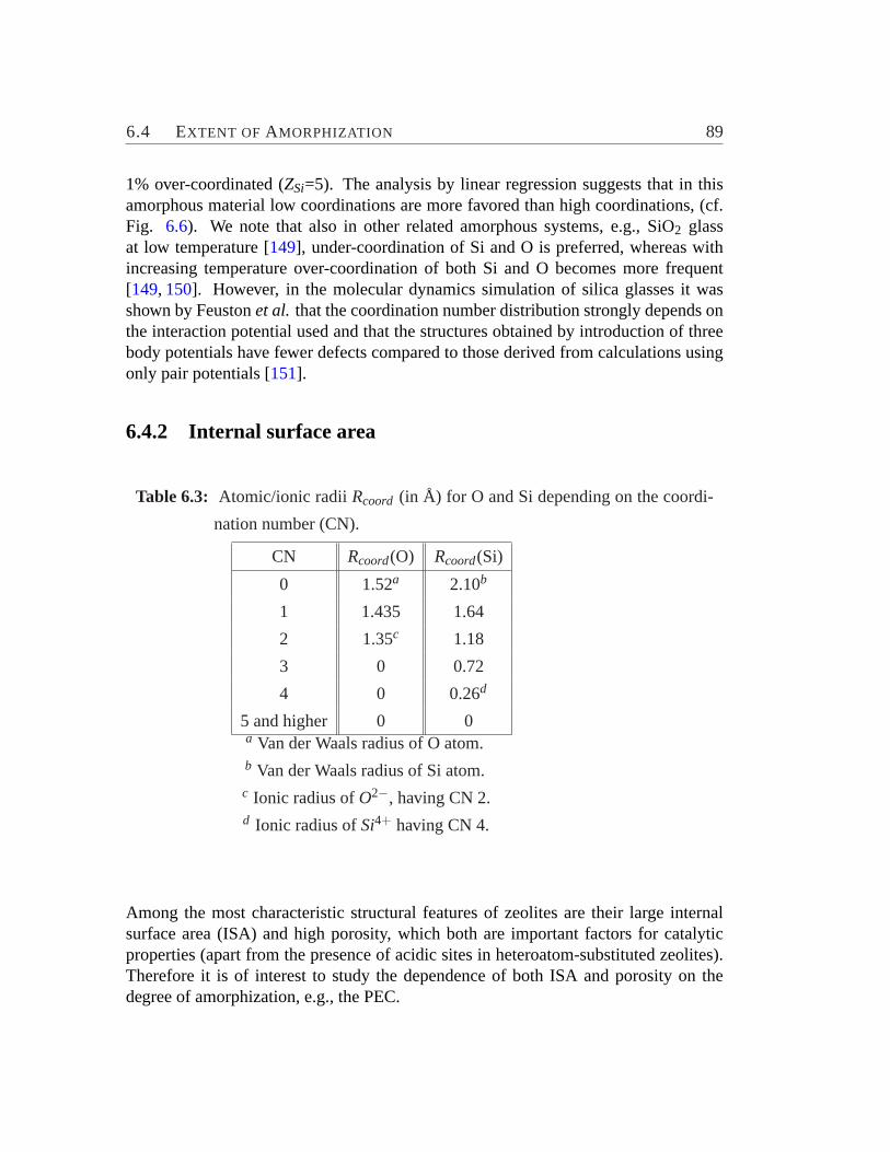
6.4 EXTENT OF AMORPHIZATION 89
1% over-coordinated (ZSi=5). The analysis by linear regression suggests that in thisamorphous material low coordinations are more favored than high coordinations, (cf.Fig. 6.6). We note that also in other related amorphous systems, e.g., SiO2 glassat low temperature [149], under-coordination of Si and O is preferred, whereas withincreasing temperature over-coordination of both Si and O becomes more frequent[149, 150]. However, in the molecular dynamics simulation of silica glasses it wasshown by Feustonet al. that the coordination number distribution strongly depends onthe interaction potential used and that the structures obtained by introduction of threebody potentials have fewer defects compared to those derived from calculations usingonly pair potentials [151].
6.4.2 Internal surface area
Table 6.3: Atomic/ionic radiiRcoord (in Å) for O and Si depending on the coordi-
nation number (CN).
CN Rcoord(O) Rcoord(Si)
0 1.52a 2.10b
1 1.435 1.64
2 1.35c 1.18
3 0 0.72
4 0 0.26d
5 and higher 0 0a Van der Waals radius of O atom.b Van der Waals radius of Si atom.c Ionic radius ofO2−, having CN 2.d Ionic radius ofSi4+ having CN 4.
Among the most characteristic structural features of zeolites are their large internalsurface area (ISA) and high porosity, which both are important factors for catalyticproperties (apart from the presence of acidic sites in heteroatom-substituted zeolites).Therefore it is of interest to study the dependence of both ISA and porosity on thedegree of amorphization, e.g., the PEC.
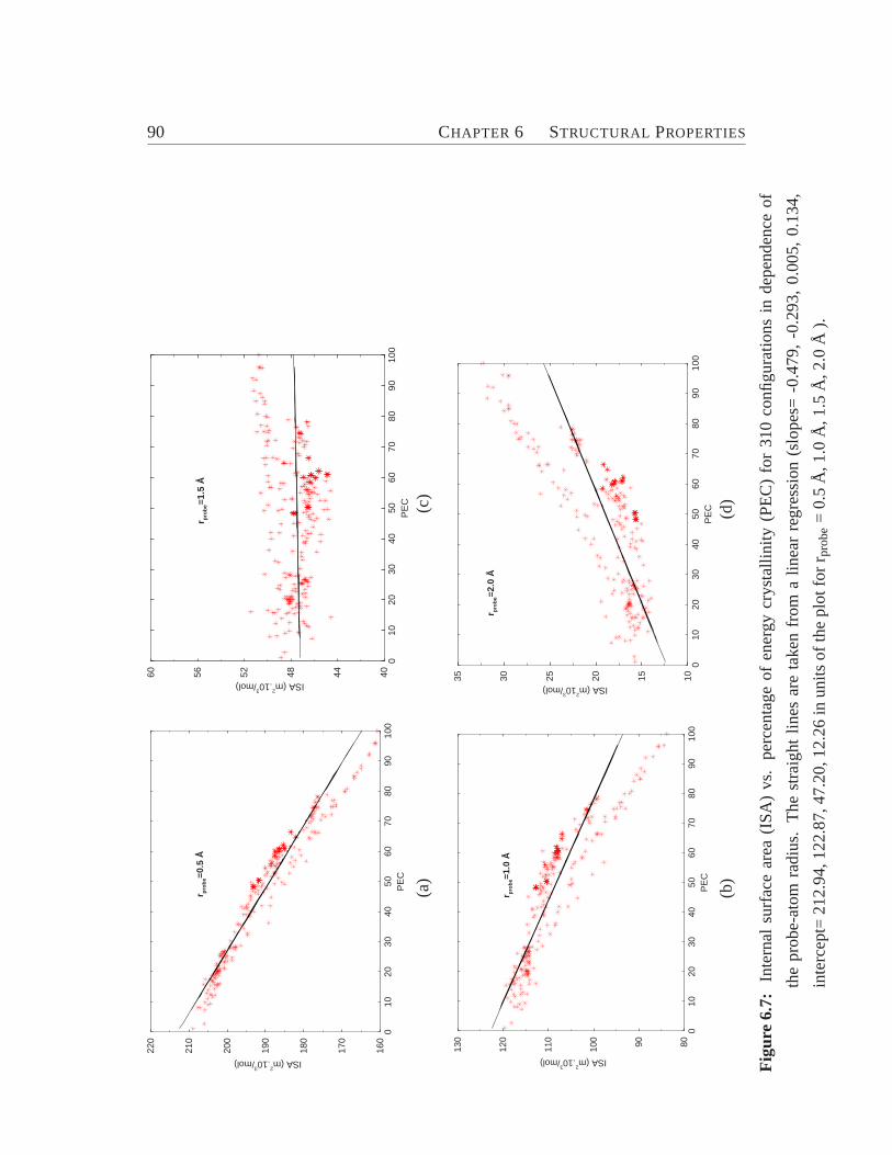
90 CHAPTER 6 STRUCTURAL PROPERTIES
010
2030
4050
6070
8090
100
PE
C
160
170
180
190
200
210
220
ISA (m2.10
3/mol)
r pro
be=
0.5
Å
010
2030
4050
6070
8090
100
PE
C
404448525660
ISA (m2.10
3/mol)
r pro
be=
1.5
Å
(a)
(c)
010
2030
4050
6070
8090
100
PE
C
8090100
110
120
130
ISA (m2.10
3/mol)
r pro
be=
1.0
Å
010
2030
4050
6070
8090
100
PE
C
101520253035ISA (m
210
3/mol)
r pro
be=
2.0
Å
(b)
(d)
Fig
ure
6.7:
Inte
rnal
surf
ace
area
(IS
A)
vs.
perc
enta
geof
ener
gycr
ysta
llini
ty(P
EC
)fo
r31
0co
nfigu
ratio
nsin
depe
nden
ceof
the
prob
e-at
omra
dius
.T
hest
raig
htlin
esar
eta
ken
from
alin
ear
regr
essi
on(s
lope
s=-0
.479
,-0
.293
,0.
005,
0.13
4,
inte
rcep
t=21
2.94
,122
.87,
47.2
0,12
.26
inun
itsof
the
plot
for
rpr
obe=
0.5
Å,1
.0Å
,1.5
Å,2
.0Å
).
6.4 EXTENT OF AMORPHIZATION 91
In order to calculate ISA we model the system as an ensemble of intersecting hardspheres with radii depending on the CN of the constituting atoms/ions. The CN ofSi/O was determined as the number of O/Si centers within a distance of 1.8 Å, i.e., allbonds contributing to the first peak in the pair-distribution functiongSi−O (Fig. 1(b))were included. Since the higher the CN of an atom/ion in the framework, the lowerits contribution to ISA, we chose the radii according to Table6.3: for uncoordinatedatoms the van der Waals radii were chosen [152], whereas for standard CN 4 for Si and2 for O the ionic radii of Si4+ and O2− were selected [153]. For intermediate valuesof the CN a linear interpolation was used. Contribution of atoms/ions with higher thanthe standard CN were neglected.
The effective ISA of a system under study depends also on the size of the probeused to measure it. A standard way to derive the effective ISA is the so-called probe-atom model, where the ISA is defined by a surface generated by the center of a hardtest sphere of radiusrprobe rolling over the ensemble of intersecting spheres [152].Recently Moloyet al. demonstrated for various crystalline zeolites that the ISA de-creases by a factor of 1.4 to 2.8 when the radius of the probe atom is increased from0.5 Å to 1.1 Å [154]. We therefore applied four different radii of the probe atom, i.e.,0.5, 1.0, 1.5 and 2.0 Å, in order to investigate the probe size dependency of the ISAupon amorphization. For the practical calculation of the ISA we increment the radii ofthe intersecting spheres described above by the probe-atom radius. The surface of theresulting ensemble of sphere was estimated as
ISA=1M
( N
∑i=1
4π[Rcoord(i)+ rprobe]2pi
p
)(6.6)
Here the sum runs over allN centersi in the MD box,Rcoord(i) refers to the atom/ionradius from Table6.3, rprobe is the probe-atom radius andM refers to the amount ofSiO2 present in the structure considered. A total ofp points (herep=614) is distributedequally on the surface of each spherei, and the numberpi of points not located insideother spheres is determined. The ratiopi/p then provides the fraction of the accessiblesurface contributed by centeri. Note that our definition of ISA does not considercases where there may be internal surfaces which are not accessible due to absenceof windows by which probe molecules can enter. Therefore, the values obtained hererepresent upper bounds to the actual accessible internal surface area.
Fig. 6.7 (a)-(d) contains our result for the ISA of 310 configurations determinedwith four different probe radii. Our values for crystalline ZSM-5, i.e., 160.77 and83.86m2· 103/mol for probe-atom radii of 0.5 and 1.0 Å, respectively, are in excellentagreement with results published by Moloyet al., i.e.,≈ 162 and≈ 84 m2· 103/mol(taken from their Fig. 7, entry MFI) [154]. Amorphization leads to a collapse of thezeolitic framework and reduces the number of big pores (cf. also the discussion ofring statistics given below). This is evident from Fig.6.7 for rprobe= 2.0 Å, whereamorphization decreases the ISA by roughly a factor of 2. However, for a small proberadius asrprobe= 0.5 Å one observes an increase of the ISA by about a factor of 2. This
92 CHAPTER 6 STRUCTURAL PROPERTIES
is explained partly by the increasing percentage of under-coordinated centers in theamorphous system (cf. Fig.6.6), but also by the increasing tendency to convert largerrings into smaller rings (cf. below). In conclusion amorphization makes the frameworkless accessible for larger species and more accessible for smaller ones. Such structuralchanges can be of high importance for catalysis, where the accessibility of the acidicsites (in case of protonated ZSM-5) and the rate of adduct-product exchange at theactive site can be the crucial parameters to influence the yield and selectivity of certainreactions [148,155]. Changes in the network topology may also result in the closureof sites suitable for ion exchange (in case of hetero-atom substituted zeolites).
6.4.3 Ring analysis
In order to gain further insight in the connectivity between the SiO4 tetrahedra and tomeasure quantitatively the effects of amorphization on the structure, e.g., the porosity,we performed a ring analysis. In the following we define a n-fold ring by the numbern of Si atoms connected by bridging O to give a ring. The number of Si atoms wasdetermined by first assigning to each bridging O atom a pair of adjacent Si atomsand then tracing possible connections to a ring containing a maximum of up to 15Si atoms. Double counting is avoided and sets of Si atoms defining a small ring arenot allowed to contribute as a whole to a large ring. Since rings can extend to periodicimages of the MD boxes the periodic boundary condition was removed for determiningthe ring distribution. The latter is sensitive to the temperature and the threshold forthe maximum distance between bonded atoms, thus configurations with similar PECcan exhibit slight differences in their ring distributions. The statistics for n-fold ringspresented in Fig.6.8 and Table6.4 nevertheless clearly shows characteristic featuresdepending on the PEC.
Crystalline ZSM-5 contains mainly 5-fold (48.9%) and 6-fold (39.2%) rings, alongwith a smaller amount of 10-fold (9.0%) and 4-fold (2.9%) rings. Amorphization isfound to lead to a broad distribution of ring sizes from 2 to 10. In 15% energy crys-talline amorphous material we observe still 5-fold (29.3%) and 6-fold (26.8%) ringsto be most frequent, however also 4-fold (17.3%) and 3-fold (13.0%) rings contributesignificantly. We can compare these findings to those from previous related work onSiO2 glass, which exhibits a pronounced dominance of 6-fold rings, i.e., 3- to 6-foldrings contribute with 3.0, 11.1, 24.2 and 61.6 %, respectively [156]. Whereas for oursystem at small PEC (as well as for the crystal) larger than 6-fold rings are present toless than 10%, they contribute with up to 20% for intermediate values of PEC. In thesecases 7-fold rings contribute roughly as much as 4-fold ones. Therefore, besides thecollapse of the 10-fold rings in crystalline ZSM-5 upon amorphization, also a "fusion"of smaller membered rings to more than 6-fold rings must occur.

6.4 EXTENT OF AMORPHIZATION 93
2 3 4 5 6 7 8 9 10Ring Size
0
10
20
30
40
50
Freq
uanc
y of
Occ
urre
nce
(%)
100 % PEC79 % PEC60 % PEC45 % PEC15 % PEC
Figure 6.8: Frequency of occurrence of n-fold rings in (partially) amorphous material
derived from ZSM-5.
The bond angle distributions suggest that both 2-fold and 3-fold rings are essen-tially planar. For 2-fold rings Si-O-Si and O-Si-O angle distributions have a peak near90◦ and for 3-fold rings Si-Si-Si and O-O-O angle distributions have a peak near60◦.This result agrees quite well with the finding of Galeener based on force-field calcu-lations that 2-fold and 3-fold rings of Si-O bonds in the vitreous form of SiO2 areexpected to be planar [157]. The presence of 2-fold rings again indicates the existenceof edge-sharing tetrahedra. However, the modest number of 2-fold rings suggests thatmost tetrahedra are linked to each other by corners.
Much more difficult than the purely topological analysis of ring sizes is their ge-ometrical measurement. Whereas small rings are essentially planar, larger ones areusually puckered considerably and make the definition of a ring diameter meaningless.Therefore, we calculate two simple measures for each ring, i.e.,
ravg =1n
n
∑i=1
i∈ring
|RSi(i)−Rc| (6.7)
and
rmin =min
i ∈ ring|RSi(i)−Rc| (6.8)
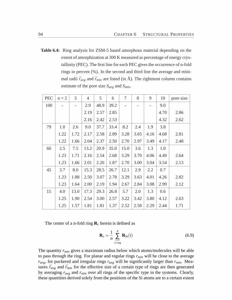
94 CHAPTER 6 STRUCTURAL PROPERTIES
Table 6.4: Ring analysis for ZSM-5 based amorphous material depending on the
extent of amorphization at 300 K measured as percentage of energy crys-
tallinity (PEC). The first line for each PEC gives the occurrence of n-fold
rings in percent (%). In the second and third line the average and mini-
mal radii ravg and rmin are listed (in Å). The rightmost column contains
estimate of the pore sizeSavg andSmin.
PEC n = 2 3 4 5 6 7 8 9 10 pore size
100 - - 2.9 48.9 39.2 - - - 9.0
2.19 2.57 2.85 4.70 2.86
2.16 2.42 2.53 4.32 2.62
79 1.0 2.6 9.0 37.7 33.4 8.2 2.4 1.9 3.8
1.22 1.72 2.17 2.58 2.89 3.28 3.65 4.16 4.68 2.81
1.22 1.66 2.04 2.37 2.50 2.70 2.97 3.49 4.17 2.48
60 2.5 7.5 13.2 20.9 35.0 15.0 3.6 1.3 1.0
1.23 1.71 2.16 2.54 2.68 3.29 3.70 4.06 4.49 2.64
1.23 1.66 2.01 2.26 1.87 2.70 3.00 3.04 3.54 2.13
45 3.7 8.0 15.3 28.5 26.7 12.1 2.9 2.2 0.7
1.23 1.88 2.50 3.07 2.78 3.29 3.63 4.01 4.26 2.82
1.23 1.64 2.00 2.19 1.94 2.67 2.84 3.08 2.99 2.12
15 4.0 13.0 17.3 29.3 26.8 5.7 2.0 1.3 0.6
1.25 1.90 2.54 3.00 2.57 3.22 3.42 3.80 4.12 2.63
1.25 1.57 1.81 1.81 1.37 2.52 2.58 2.29 2.44 1.71
The center of a n-fold ringRc herein is defined as
Rc =1n
n
∑i=1
i∈ring
RSi(i) (6.9)
The quantityrmin gives a maximum radius below which atoms/molecules will be ableto pass through the ring. For planar and regular ringsrmin will be close to the averageravg, for puckered and irregular ringsravg will be significantly larger thanrmin. Mea-suresravg and rmin for the effective size of a certain type of rings are then generatedby averagingravg andrmin over all rings of the specific type in the systems. Clearly,these quantities derived solely from the positions of the Si atoms are to a certain extent
6.4 EXTENT OF AMORPHIZATION 95
arbitrary. In reality the effective ring size depends not only on the electron densitydistribution of the Si and O atoms in the ring but also on the one of the probe system.In addition vibrational motion will affect the effective ring size. Summing up, a welldefined unique probe-independent measure of ring size cannot be given, neverthelesswe believe that the values ofravg and rmin listed also in Table6.4 provide reasonabletrends.
For crystalline ZSM-5 the values ofravg andrmin are quite similar with a maximumdeviation of≈ 13%for 6-fold rings. With increasing degree of amorphization the ratioravg/rmin increases up to almost a factor of two for some ring sizes, i.e.,≈1.9 for 6-foldand≈1.7 for 5-,9- and 10-fold rings. This indicates that the most frequently occurringring types (5- and 6-fold) have the largest tendency to irregular shape and puckering,leading to smaller effective pore sizes in amorphous systems.
From the individual ring averagesravg andrmin we can derive global averagesSavg
andSmin for the amorphous system (cf. the right column in Table6.4) by weighting thering-specific valuesravg and rmin with the occurrence of the ring types. These shouldhave some relation to measured effective pore sizes. Whereas the averaged valueSavg
does not exhibit a clear trend with decreasing PEC, the averageSmin clearly decreases.This finding is in line with the concomitant decrease of ISA for large probe-atomsdepicted in Fig.6.7. We conclude thatSmin might be more helpful in the discussion ofcatalytic processes. Finally we want to mention that despite all reservation the orderof magnitude ofSmin appears to be realistic: for crystalline ZSM-5 we estimate aneffective pore diameter of at least 5.2 Å. This agrees well with the value of around 5.5Å of the micropore size distribution by Saitoet al. obtained experimentally from highresolution argon adsorption on ZSM-5 [158].
This part of the work is published in Ref. [159]


Chapter 7
Vibrational Properties
Experimental studies on the mechanical treatment of zeolites by ball-milling processesshow that the amorphization also causes remarkable changes in the vibrational infrared(IR) spectra which were associated with the breaking of Si-O-Si bonds [19,20]. It wassuggested that certain characteristic bands could be used as probes for detecting theextent of the presence of the zeolite framework [160]. In the following section, adetailed investigation of vibrational properties of amorphous materials derived fromthe silicious ZSM-5 is presented.
7.1 Vibrational Density of States
The absence of a periodic lattice in amorphous materials has several effects; an im-mediate consequence is that there is no reciprocal lattice and sok is no longer a goodquantum number for excitations in the solid, such as phonons (as described in chapter 4section (4.2.3)). Thus phonon states cannot de described in terms of dispersion curves,instead the only quantity which is a valid description of excitations in a non-crystallinesolid is the "density of states" (DOS).
The dependence of many thermodynamic properties, e.g., the specific heatCV , onvibrational motions, makes the vibrational DOS a crucial property of solids. Experi-mentally it can be measured with inelastic neutron scattering as well as IR and Ramanspectroscopy. In the following we present calculations of the vibrational DOS obtainedby two theoretical methods, i.e., the diagonalization of the dynamic matrix and theFourier transformation of the velocity-autocorrelation function [161,162]. Numericalcalculations of the vibrational DOS by the diagonalization of the dynamic matrix arebased on the harmonic approximation of the potential energy, allow an analysis of thevibrational modes, but neglect anharmonicities as well as temperature effects. Usingthe second method proposed above, one is able to study the temperature dependenceof the vibrational and thermodynamic properties of the solids. However, this method
97
98 CHAPTER 7 VIBRATIONAL PROPERTIES
suffers from the finite resolution of frequencies and the lack of information about theeigenmodes of the structures.
A detailed description of the structure generation is given in Chapter 6. In all20 structures each comprising of 1152 particles were generated. After quenching thelow-temperature configurations, i.e., the ones obtained at 300 K, a final quenchingto 0 K leading to the local minima of the potential energy surface was performed. Inthese minima we calculated the dynamic matrix whose elements are the mass-weightedsecond derivatives of the potential energyU with respect to the atomic positions
Dmnαβ =
1√MnMm
∂2U(Rm−Rn)∂Rm
α ∂Rnβ
,
m,n = [1,2, ...,N],α,β = [x,y,z]. (7.1)
HereMn represents the mass of thenth atom andRnα is the coordinate of atomn in α
direction. Diagonalization of the dynamic matrix gives 3N eigenvalues correspondingto the square of the eigenfrequencies (ω2, whereω = 2πν) and real eigenvectors (e).Among the 3N vibrational modes the contributions by the three translation modes arealmost negligible. The vibrational DOS is obtained from the frequenciesν j of 3N-3vibrational and rotational modesj as
Z(ν) =⟨ 1
3N−3∑j
δ(ν−ν j)⟩, (7.2)
whereδ is the discretized delta function and⟨...
⟩stands for an ensemble average. Due
to the small system size the low-frequency part (below 0.7 THz) could not be obtainedand hence we calculated the Debye spectrum given by
ZDebye=3
ν3D
ν2, (7.3)
with
νD = c( 3N
4πV
)1/3. (7.4)
Here c represents the average sound velocity given in terms of the longitudinal andtransverse velocitiescl andct , respectively.N/V is the number density of the system.We use the fact of the isotropy of amorphous materials and calculated these velocitiesfrom the elastic constants ascl =
√c11/ρ and ct =
√c44/ρ, whereρ is the mass
density of the system. These values of the elastic constants were obtained from thechanges in the potential energy∆E under an applied strain
Rmα → Rm
α +∑β
εαβRmβ , (7.5)
∆E =−∑αβ
Pαβεαβ +V2 ∑
αβγδεαβCαβγδεγδ +
12 ∑
αβγPαβεαγεγβ. (7.6)
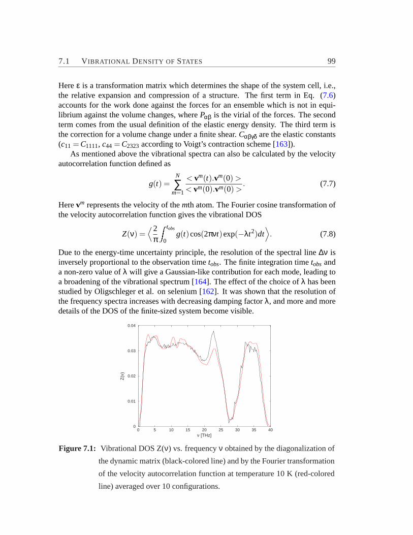
7.1 VIBRATIONAL DENSITY OF STATES 99
Hereε is a transformation matrix which determines the shape of the system cell, i.e.,the relative expansion and compression of a structure. The first term in Eq. (7.6)accounts for the work done against the forces for an ensemble which is not in equi-librium against the volume changes, wherePαβ is the virial of the forces. The secondterm comes from the usual definition of the elastic energy density. The third term isthe correction for a volume change under a finite shear.Cαβγδ are the elastic constants(c11 = C1111, c44 = C2323 according to Voigt’s contraction scheme [163]).
As mentioned above the vibrational spectra can also be calculated by the velocityautocorrelation function defined as
g(t) =N
∑m=1
< vm(t).vm(0) >
< vm(0).vm(0) >. (7.7)
Herevm represents the velocity of themth atom. The Fourier cosine transformation ofthe velocity autocorrelation function gives the vibrational DOS
Z(ν) =⟨2
π
Z tobs
0g(t)cos(2πνt)exp(−λt2)dt
⟩. (7.8)
Due to the energy-time uncertainty principle, the resolution of the spectral line∆ν isinversely proportional to the observation timetobs. The finite integration timetobs anda non-zero value ofλ will give a Gaussian-like contribution for each mode, leading toa broadening of the vibrational spectrum [164]. The effect of the choice ofλ has beenstudied by Oligschleger et al. on selenium [162]. It was shown that the resolution ofthe frequency spectra increases with decreasing damping factorλ, and more and moredetails of the DOS of the finite-sized system become visible.
0 5 10 15 20 25 30 35 40ν [THz]
0
0.01
0.02
0.03
0.04
Z(ν
)
Figure 7.1: Vibrational DOS Z(ν) vs. frequencyν obtained by the diagonalization of
the dynamic matrix (black-colored line) and by the Fourier transformation
of the velocity autocorrelation function at temperature 10 K (red-colored
line) averaged over 10 configurations.

100 CHAPTER 7 VIBRATIONAL PROPERTIES
Fig. 7.1 shows the vibrational density of statesZ(ν) obtained by both the abovementioned methods for the ten structures with an average PEC of 50 %, which is asubset of the 20 generated configurations of partially crystalline forms. In the collec-tion of ten such structures the lowest and highest value of PEC taken into account was47 % and 52%, respectively. In order to obtain the vibrational density of states by theFourier transformation of the velocity autocorrelation function, the equations of mo-tions were integrated with a time step of 0.1 fs for a time intervaltobs=1.00 ps. Ten setsof initial conditions with a temperature of 10 K and a damping factorλ =4/t2
obs werechosen. The overall shapes of the spectra are very similar. Details, e.g., more or lesspronounced peaks observed for the Fourier Cosine Transformation depend on the num-ber of sampled systems, the choice ofλ and the length of the observation time [162].In contrast to the diagonalization of the dynamic matrix the approach also accounts forrelaxation and temperature effects, i.e., a complete agreement is not to be expected.The elastic constantsc11 andc44 are found to be 7.03×10¹⁰ N/m2 and 5.77×10¹⁰
N/m2, respectively, for the systems with the mass density of 1.785 g/cm3. Hence thecalculated sound velocitiescl andct are 6275 m/s and 5687 m/s, respectively. Thepercentage of anisotropy seen in terms of elastic constants in the system is found tobe less than 7%, hence, the system can be considered to be isotropic for all practicalpurpose. At this point we want to mention that we also calculated the sound velocitiescl andct using potentials designed by Vashishta [165]. We obtain the values 5181 m/sand 3358 m/s forcl andct , respectively. Despite of yielding a good description for thestructural [159,124] and vibrational [127] properties, it was shown that the potentialby Krameret al. used in the present simulation, yields somewhat less accurate elasticproperties in zeolite [124]. For sodalite the values ofc11, c44, c12 were overestimatedby 30%, 8% and 72%, respectively. As a consequence the values obtained for thesound velocities in our simulation also seem to be at the higher end. Neverthelesswe decided to use the potential of Krameret al. since it yielded the experimentallyobserved characteristic structure of the high-energy spectrum of silica [127], whereasthis is not the case for the one of Vashishtaet al. [149].
In Fig. 7.2 we analyzed the motion of single elements and their contribution tothe vibrational DOS obtained by the Fourier transformation of the element-specificvelocity autocorrelation function given by
ZA(ν) =⟨2
π
Z tobs
0gA(t)cos(2πνt)exp(−λt2)dt
⟩(7.9)
where
gA(t) =NA
∑n=1
< vA(t).vA(0) >
< vA(0).vA(0) >. (7.10)
HereNA represents the number of atoms of typeA. It is easy to see that the motionsof oxygen atoms contribute dominantly for all frequency regions in the vibrationalDOS. Nevertheless, the contributions of the silicon atoms become quite significantand comparable in magnitude for a peak in the mid-frequency region, i.e., around 24

7.2 ANALYSIS OF THE V IBRATIONAL MODES 101
THz. By MD simulations of silica glasses it was shown that the contribution of thesilicon atoms even exceeds that of the oxygen atoms for this particular peak [149].
0 5 10 15 20 25 30 35 40ν [THz]
0
0.01
0.02
0.03
0.04
0.05
Z (
ν)TotalSiliconOxygen
Figure 7.2: Averaged element specific-contribution to the total vibrational DOS for
10 configurations with an average PEC of 50% obtained by the Fourier
transformation of the velocity autocorrelation function. Total vibrational
DOS (black-colored line), Si contribution (red-colored line) and O contri-
bution (blue-colored line) are plotted versus frequency in THz.
The best known anomalous low-temperature property of amorphous materials istheir specific heat as mentioned in Chapter 4. In crystals the observed specific heatis directly proportional toT3 and the proportionality constant is determined by thevelocities of sound. In an amorphous system due to the presence of additional modesone observes deviations from this behavior. In the harmonic approximationCV peratom is expressed in terms of the DOS as given in Eq. (4.34). In Fig. 7.3 we plottedthe specific heat asCV/T3 as a function of temperatureT. The dashed line shows thevalues obtained for the spectrum by adding the Debye contribution up to a frequencysmaller than the lowest possible vibrational frequency seen in our system, i.e., 0.7 THz.This correction amounts to 1.8× 10⁻³ of all the modes.
7.2 Analysis of the Vibrational Modes
7.2.1 Element specific motion with respect to bonds
In Fig. 7.2 the relative contributions of oxygen and silicon atoms to the vibrationalDOS is presented. To learn about the typical motions of these components we calcu-lated the angle between the displacement of atomi in mode j and the bond of this atom
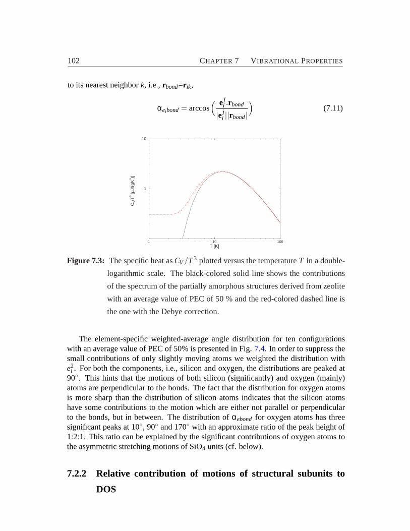
102 CHAPTER 7 VIBRATIONAL PROPERTIES
to its nearest neighbork, i.e.,rbond=r ik,
αeibond = arccos( ej
i .rbond
|eji ||rbond|
)(7.11)
1 10 100T [K]
1
10
CV/T
3 [µJ/
(gK
4 )]
Figure 7.3: The specific heat asCV/T3 plotted versus the temperatureT in a double-
logarithmic scale. The black-colored solid line shows the contributions
of the spectrum of the partially amorphous structures derived from zeolite
with an average value of PEC of 50 % and the red-colored dashed line is
the one with the Debye correction.
The element-specific weighted-average angle distribution for ten configurationswith an average value of PEC of 50% is presented in Fig.7.4. In order to suppress thesmall contributions of only slightly moving atoms we weighted the distribution withe2
i . For both the components, i.e., silicon and oxygen, the distributions are peaked at90◦. This hints that the motions of both silicon (significantly) and oxygen (mainly)atoms are perpendicular to the bonds. The fact that the distribution for oxygen atomsis more sharp than the distribution of silicon atoms indicates that the silicon atomshave some contributions to the motion which are either not parallel or perpendicularto the bonds, but in between. The distribution ofαebond for oxygen atoms has threesignificant peaks at 10◦, 90◦ and 170◦ with an approximate ratio of the peak height of1:2:1. This ratio can be explained by the significant contributions of oxygen atoms tothe asymmetric stretching motions of SiO4 units (cf. below).
7.2.2 Relative contribution of motions of structural subunits to
DOS
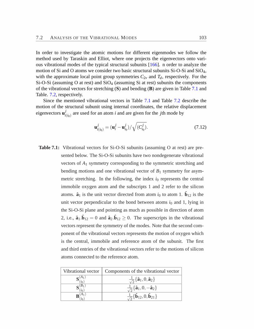
7.2 ANALYSIS OF THE V IBRATIONAL MODES 103
In order to investigate the atomic motions for different eigenmodes we follow themethod used by Taraskin and Elliot, where one projects the eigenvectors onto vari-ous vibrational modes of the typical structural subunits [166]. n order to analyze themotion of Si and O atoms we consider two basic structural subunits Si-O-Si and SiO4,with the approximate local point group symmetriesC2v andTd, respectively. For theSi-O-Si (assuming O at rest) and SiO4 (assuming Si at rest) subunits the componentsof the vibrational vectors for stretching (S) and bending (B) are given in Table7.1andTable.7.2, respectively.
Since the mentioned vibrational vectors in Table7.1 and Table7.2 describe themotion of the structural subunit using internal coordinates, the relative displacementeigenvectorsu j
i(i0)are used for an atomi and are given for thejth mode by
u ji(i0)
= (u ji −u j
i0)/
√(C j
i0). (7.12)
Table 7.1: Vibrational vectors for Si-O-Si subunits (assuming O at rest) are pre-
sented below. The Si-O-Si subunits have two nondegenerate vibrational
vectors ofA1 symmetry corresponding to the symmetric stretching and
bending motions and one vibrational vector ofB1 symmetry for asym-
metric stretching. In the following, the indexi0 represents the central
immobile oxygen atom and the subscripts 1 and 2 refer to the silicon
atoms.a1 is the unit vector directed from atomi0 to atom 1.b12 is the
unit vector perpendicular to the bond between atomsi0 and 1, lying in
the Si-O-Si plane and pointing as much as possible in direction of atom
2, i.e., a1.b12 = 0 and a2.b12 ≥ 0. The superscripts in the vibrational
vectors represent the symmetry of the modes. Note that the second com-
ponent of the vibrational vectors represents the motion of oxygen which
is the central, immobile and reference atom of the subunit. The first
and third entries of the vibrational vectors refer to the motions of silicon
atoms connected to the reference atom.
Vibrational vector Components of the vibrational vector
S(A1)(i0)
1√2{a1,0, a2}
S(B1)(i0)
1√2{a1,0,−a2}
B(A1)(i0)
1√2{b12,0, b21}
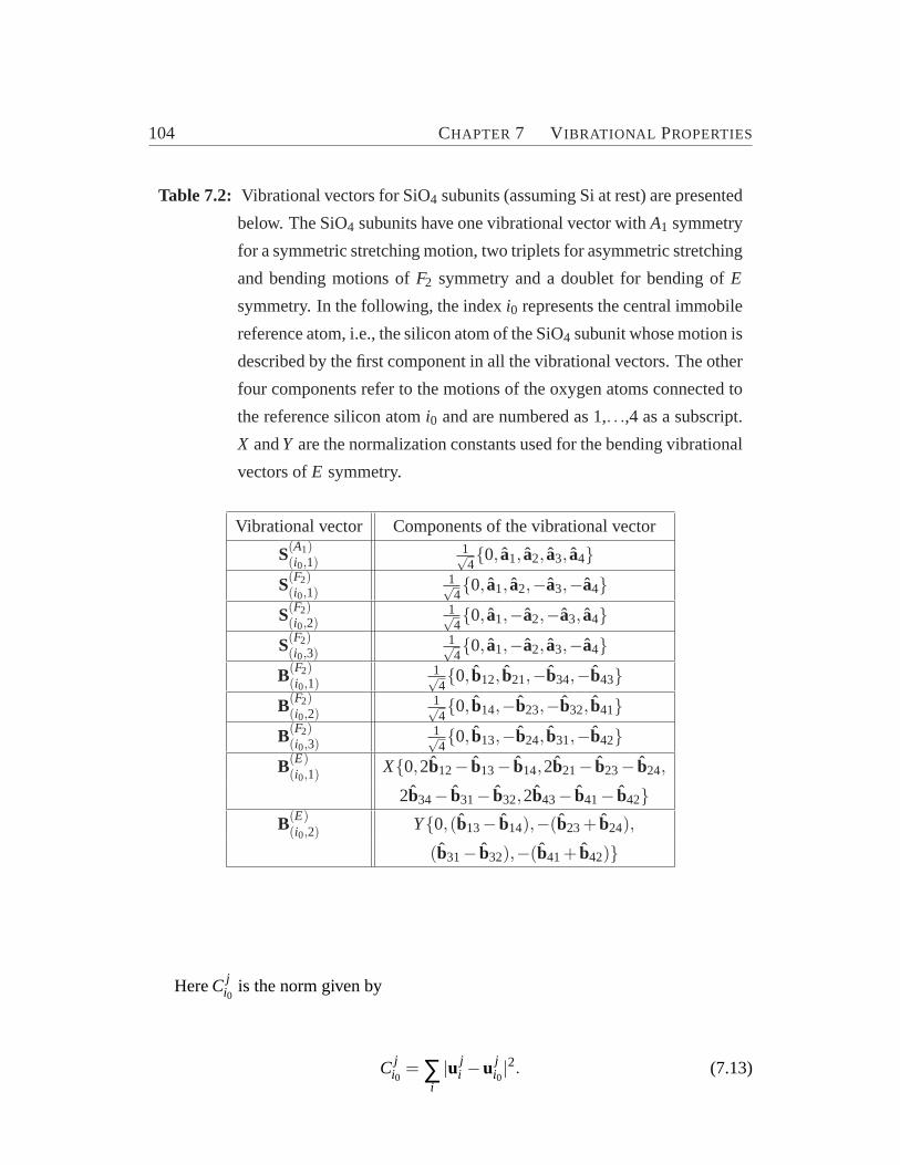
104 CHAPTER 7 VIBRATIONAL PROPERTIES
Table 7.2: Vibrational vectors for SiO4 subunits (assuming Si at rest) are presented
below. The SiO4 subunits have one vibrational vector withA1 symmetry
for a symmetric stretching motion, two triplets for asymmetric stretching
and bending motions ofF2 symmetry and a doublet for bending ofE
symmetry. In the following, the indexi0 represents the central immobile
reference atom, i.e., the silicon atom of the SiO4 subunit whose motion is
described by the first component in all the vibrational vectors. The other
four components refer to the motions of the oxygen atoms connected to
the reference silicon atomi0 and are numbered as 1,. . .,4 as a subscript.
X andY are the normalization constants used for the bending vibrational
vectors ofE symmetry.
Vibrational vector Components of the vibrational vector
S(A1)(i0,1)
1√4{0, a1, a2, a3, a4}
S(F2)(i0,1)
1√4{0, a1, a2,−a3,−a4}
S(F2)(i0,2)
1√4{0, a1,−a2,−a3, a4}
S(F2)(i0,3)
1√4{0, a1,−a2, a3,−a4}
B(F2)(i0,1)
1√4{0, b12, b21,−b34,−b43}
B(F2)(i0,2)
1√4{0, b14,−b23,−b32, b41}
B(F2)(i0,3)
1√4{0, b13,−b24, b31,−b42}
B(E)(i0,1) X{0,2b12− b13− b14,2b21− b23− b24,
2b34− b31− b32,2b43− b41− b42}B(E)
(i0,2) Y{0,(b13− b14),−(b23+ b24),
(b31− b32),−(b41+ b42)}
HereC ji0
is the norm given by
C ji0
= ∑i|u j
i −u ji0|2. (7.13)

7.2 ANALYSIS OF THE V IBRATIONAL MODES 105
0 20 40 60 80 100 120 140 160 180αebond [deg]
0
0.02
0.04
0.06
0.08
D(α
ebon
d)
Figure 7.4: Distribution of element-specific weighted-average anglesαebondbetween
the atomic displacement eigenvectors and the bonds. The black-colored
solid line corresponds to the angle distribution of silicon atoms and the
red-colored dashed line to the one of oxygen atoms for ten configurations
with an average value of PEC 50%.
The displacement eigenvectorsu ji are derived from the eigenvectorsej
i as u ji =
eji /√
Mi with the massMi of the ith atom. Herei0 represents the central, immobile,reference atom for the structural subunits. The squared value of the projection of therelative displacement eigenvectoru j
i(I ,i0)onto the vibrational vectorsDi(I) (S’s andB’s
in Table7.1and Table7.2) of the structural subunitI gives the partial contribution ofthe vibrational motion of a specific kind for the eigenmodej. These squared projec-tions were averaged over all structural subunits as
(r jD)2 =
∑I (wjI )
2(∑i′(I) u ji′(I ,i0)
.Di′(I))2
∑I (wjI )2
. (7.14)
Here the indexI runs over all the structural units, i.e., Si-O-Si or SiO4, and the indexi′runs over all the atoms comprising the structural subunit.The weighting factorw j
I isused in order to suppress the contributions of units which have negligible values andis given by
w jI =
(∑i′|ej
i′|2
)1/2. (7.15)
In order to obtain the rotational component of the spectrum, we obtain three perpendic-ular axes for a given subunit as eigenvectors by diagonalizing the shape tensor givenby
Gαβ(i0) = ∑i′
Mi′ rαi0i′r
βi0i′ . (7.16)
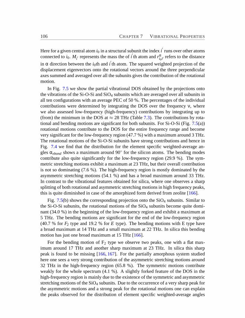
106 CHAPTER 7 VIBRATIONAL PROPERTIES
Here for a given central atomi0 in a structural subunit the indexi′runs over other atoms
connected toi0. Mi′ represents the mass the ofi′th atom andrα
i0i′ refers to the distance
in α direction between thei0th andi′th atom. The squared weighted projection of the
displacement eigenvectors onto the rotational vectors around the three perpendicularaxes summed and averaged over all the subunits gives the contribution of the rotationalmotion.
In Fig. 7.5 we show the partial vibrational DOS obtained by the projections ontothe vibrations of the Si-O-Si and SiO4 subunits which are averaged over all subunits inall ten configurations with an average PEC of 50 %. The percentages of the individualcontributions were determined by integrating the DOS over the frequencyν, wherewe also assessed low-frequency (high-frequency) contributions by integrating up to(from) the minimum in the DOS at≈ 28 THz (Table7.3). The contributions by rota-tional and bending motions are significant for both subunits. For Si-O-Si (Fig.7.5(a))rotational motions contribute to the DOS for the entire frequency range and becomevery significant for the low-frequency region (47.7 %) with a maximum around 3 THz.The rotational motions of the Si-O-Si subunits have strong contributions and hence inFig. 7.4 we find that the distribution for the element specific weighted-average an-glesαebondshows a maximum around 90◦ for the silicon atoms. The bending modescontribute also quite significantly for the low-frequency region (29.9 %). The sym-metric stretching motions exhibit a maximum at 23 THz, but their overall contributionis not so dominating (7.6 %). The high-frequency region is mostly dominated by theasymmetric stretching motions (54.1 %) and has a broad maximum around 33 THz.In contrast to the vibrational features obtained for silica, where one observes a sharpsplitting of both rotational and asymmetric stretching motions in high frequency peaks,this is quite diminished in case of the amorphized form derived from zeolite [166].
Fig. 7.5(b) shows the corresponding projection onto the SiO4 subunits. Similar tothe Si-O-Si subunits, the rotational motions of the SiO4 subunits become quite domi-nant (34.0 %) in the beginning of the low-frequency region and exhibit a maximum at5 THz. The bending motions are significant for the end of the low-frequency region(40.7 % forF2 type and 19.2 % forE type). The bending motions with E type havea broad maximum at 14 THz and a small maximum at 22 THz. In silica this bendingmotion has just one broad maximum at 15 THz [166].
For the bending motion of F2 type we observe two peaks, one with a flat max-imum around 17 THz and another sharp maximum at 23 THz. In silica this sharppeak is found to be missing [166, 167]. For the partially amorphous system studiedhere one sees a very strong contribution of the asymmetric stretching motions around32 THz in the high-frequency region (65.8 %). The symmetric motions contributeweakly for the whole spectrum (4.1 %). A slightly forked feature of the DOS in thehigh-frequency region is mainly due to the existence of the symmetric and asymmetricstretching motions of the SiO4 subunits. Due to the occurrence of a very sharp peak forthe asymmetric motions and a strong peak for the rotational motions one can explainthe peaks observed for the distribution of element specific weighted-average angles

7.2 ANALYSIS OF THE V IBRATIONAL MODES 107
0 5 10 15 20 25 30 35 40ν [THz]
0
5
10
15
20
25
30
35Z
(ν)
Tot.
Rot.
Asym.
Bend.
Sym.
(a)
0 5 10 15 20 25 30 35 40ν [THz]
0
5
10
15
20
25
30
35
Z(ν
)
Tot.
Rot. Asym.
Sym.
Bend.(F2)
Bend.(E)
(b)
Figure 7.5: (a) The total and partial vibrational DOS obtained by the projection of the
relative atomic displacements onto the vibrational vectors of the (a) Si-O-
Si and (b) SiO4 subunits. All the plots are shown as an average over 10
configurations with an average value of PEC of 50 %.
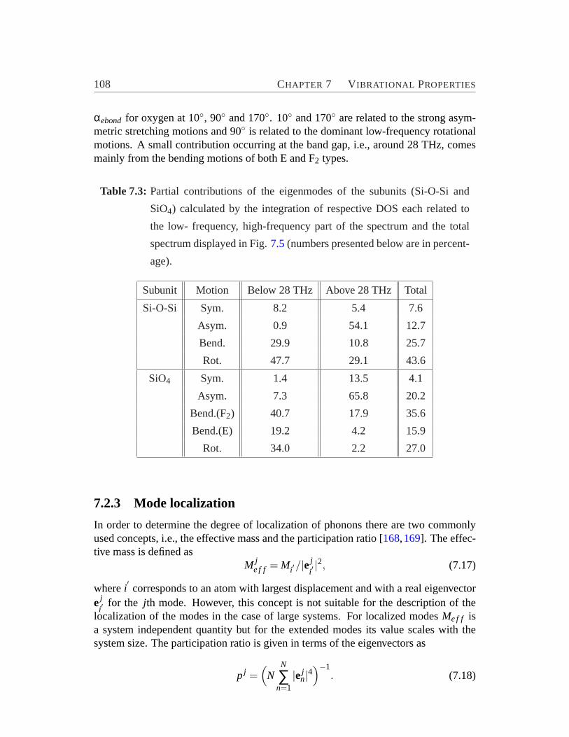
108 CHAPTER 7 VIBRATIONAL PROPERTIES
αebond for oxygen at 10◦, 90◦ and 170◦. 10◦ and 170◦ are related to the strong asym-metric stretching motions and 90◦ is related to the dominant low-frequency rotationalmotions. A small contribution occurring at the band gap, i.e., around 28 THz, comesmainly from the bending motions of both E and F2 types.
Table 7.3: Partial contributions of the eigenmodes of the subunits (Si-O-Si and
SiO4) calculated by the integration of respective DOS each related to
the low- frequency, high-frequency part of the spectrum and the total
spectrum displayed in Fig.7.5(numbers presented below are in percent-
age).
Subunit Motion Below 28 THz Above 28 THz Total
Si-O-Si Sym. 8.2 5.4 7.6
Asym. 0.9 54.1 12.7
Bend. 29.9 10.8 25.7
Rot. 47.7 29.1 43.6
SiO4 Sym. 1.4 13.5 4.1
Asym. 7.3 65.8 20.2
Bend.(F2) 40.7 17.9 35.6
Bend.(E) 19.2 4.2 15.9
Rot. 34.0 2.2 27.0
7.2.3 Mode localization
In order to determine the degree of localization of phonons there are two commonlyused concepts, i.e., the effective mass and the participation ratio [168,169]. The effec-tive mass is defined as
M je f f = Mi′/|e
ji′|2, (7.17)
wherei′corresponds to an atom with largest displacement and with a real eigenvector
eji′
for the jth mode. However, this concept is not suitable for the description of thelocalization of the modes in the case of large systems. For localized modesMe f f isa system independent quantity but for the extended modes its value scales with thesystem size. The participation ratio is given in terms of the eigenvectors as
p j =(
NN
∑n=1
|ejn|4
)−1. (7.18)
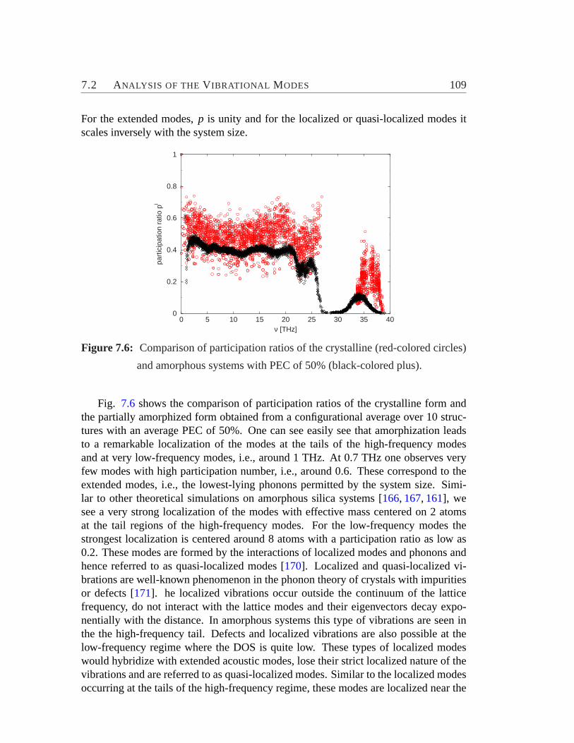
7.2 ANALYSIS OF THE V IBRATIONAL MODES 109
For the extended modes,p is unity and for the localized or quasi-localized modes itscales inversely with the system size.
0 5 10 15 20 25 30 35 40ν [THz]
0
0.2
0.4
0.6
0.8
1pa
rtic
ipat
ion
ratio
pj
Figure 7.6: Comparison of participation ratios of the crystalline (red-colored circles)
and amorphous systems with PEC of 50% (black-colored plus).
Fig. 7.6 shows the comparison of participation ratios of the crystalline form andthe partially amorphized form obtained from a configurational average over 10 struc-tures with an average PEC of 50%. One can see easily see that amorphization leadsto a remarkable localization of the modes at the tails of the high-frequency modesand at very low-frequency modes, i.e., around 1 THz. At 0.7 THz one observes veryfew modes with high participation number, i.e., around 0.6. These correspond to theextended modes, i.e., the lowest-lying phonons permitted by the system size. Simi-lar to other theoretical simulations on amorphous silica systems [166, 167, 161], wesee a very strong localization of the modes with effective mass centered on 2 atomsat the tail regions of the high-frequency modes. For the low-frequency modes thestrongest localization is centered around 8 atoms with a participation ratio as low as0.2. These modes are formed by the interactions of localized modes and phonons andhence referred to as quasi-localized modes [170]. Localized and quasi-localized vi-brations are well-known phenomenon in the phonon theory of crystals with impuritiesor defects [171]. he localized vibrations occur outside the continuum of the latticefrequency, do not interact with the lattice modes and their eigenvectors decay expo-nentially with the distance. In amorphous systems this type of vibrations are seen inthe the high-frequency tail. Defects and localized vibrations are also possible at thelow-frequency regime where the DOS is quite low. These types of localized modeswould hybridize with extended acoustic modes, lose their strict localized nature of thevibrations and are referred to as quasi-localized modes. Similar to the localized modesoccurring at the tails of the high-frequency regime, these modes are localized near the
110 CHAPTER 7 VIBRATIONAL PROPERTIES
defects. However, their eigenvectors do not decay exponentially [98].Similar to the analysis of Jinet al. we calculated the effective radius of gyration
Rjgyr for the jth mode as
Rjgyr =
√13∑
α[< Xα( j)2 >−< Xα( j) >2], (7.19)
where
< Xα( j)2 >=N
∑i=1|ej
iα|2(r iα − r i′α)2 (7.20)
and
< Xα( j) >=N
∑i=1|ej
iα |2(r iα − r i′α). (7.21)
Herei′refers to an atom with the largest displacement for thejth mode. For a localized
mode involving essentially only the motion of a single atomRgyr will be zero and foran extended mode it is the average root-mean-squared distance [161]. Fig. 7.7showsRgyr/L for various frequencies. The average box lengthL is 28.8 Å. The average radiusof gyration for the quasi-localized low-frequency modes are approximately 0.3 timesof the box length. However, for the high-frequency region the modes especially at thetails become highly localized, i.e., within 0.01 times the box length.
0 5 10 15 20 25 30 35 40ν [THz]
0
0.1
0.2
0.3
0.4
radi
us o
f gyr
atio
n R
gyrj /L
Figure 7.7: Plot of radius of gyration asRgyr/L versus frequency with L as length of
the simulation box.
7.2.4 Phase quotient
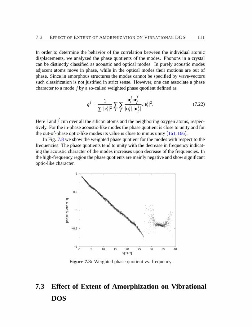
7.3 EFFECT OFEXTENT OF AMORPHIZATION ON V IBRATIONAL DOS 111
In order to determine the behavior of the correlation between the individual atomicdisplacements, we analyzed the phase quotients of the modes. Phonons in a crystalcan be distinctly classified as acoustic and optical modes. In purely acoustic modesadjacent atoms move in phase, while in the optical modes their motions are out ofphase. Since in amorphous structures the modes cannot be specified by wave-vectorssuch classification is not justified in strict sense. However, one can associate a phasecharacter to a modej by a so-called weighted phase quotient defined as
q j =1
∑i |eji |2
∑i
∑i′
u ji .u
ji′
|u ji |.|u j
i′|.|ej
i |2. (7.22)
Herei andi′run over all the silicon atoms and the neighboring oxygen atoms, respec-
tively. For the in-phase acoustic-like modes the phase quotient is close to unity and forthe out-of-phase optic-like modes its value is close to minus unity [161,166].
In Fig. 7.8we show the weighted phase quotient for the modes with respect to thefrequencies. The phase quotients tend to unity with the decrease in frequency indicat-ing the acoustic character of the modes increases upon decrease of the frequencies. Inthe high-frequency region the phase quotients are mainly negative and show significantoptic-like character.
0 5 10 15 20 25 30 35 40ν[THz]
−1
−0.5
0
0.5
1
phas
e qu
otie
nt q
j
Figure 7.8: Weighted phase quotient vs. frequency.
7.3 Effect of Extent of Amorphization on Vibrational
DOS
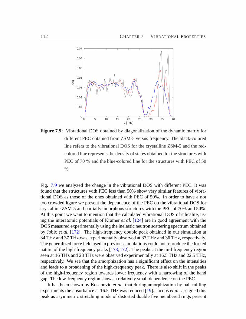
112 CHAPTER 7 VIBRATIONAL PROPERTIES
0 5 10 15 20 25 30 35 40ν [THz]
0
0.01
0.02
0.03
0.04
0.05
0.06
0.07
Z(ν
)
Figure 7.9: Vibrational DOS obtained by diagonalization of the dynamic matrix for
different PEC obtained from ZSM-5 versus frequency. The black-colored
line refers to the vibrational DOS for the crystalline ZSM-5 and the red-
colored line represents the density of states obtained for the structures with
PEC of 70 % and the blue-colored line for the structures with PEC of 50
%.
Fig. 7.9 we analyzed the change in the vibrational DOS with different PEC. It wasfound that the structures with PEC less than 50% show very similar features of vibra-tional DOS as those of the ones obtained with PEC of 50%. In order to have a nottoo crowded figure we present the dependence of the PEC on the vibrational DOS forcrystalline ZSM-5 and partially amorphous structures with the PEC of 70% and 50%.At this point we want to mention that the calculated vibrational DOS of silicalite, us-ing the interatomic potentials of Krameret al. [124] are in good agreement with theDOS measured experimentally using the inelastic neutron scattering spectrum obtainedby Jobicet al. [172]. The high-frequency double peak obtained in our simulation at34 THz and 37 THz was experimentally observed at 33 THz and 36 THz, respectively.The generalized force field used in previous simulations could not reproduce the forkednature of the high-frequency peaks [173,172]. The peaks at the mid-frequency regionseen at 16 THz and 23 THz were observed experimentally at 16.5 THz and 22.5 THz,respectively. We see that the amorphization has a significant effect on the intensitiesand leads to a broadening of the high-frequency peak. There is also shift in the peaksof the high-frequency region towards lower frequency with a narrowing of the bandgap. The low-frequency region shows a relatively small dependence on the PEC.
It has been shown by Kosanovicet al. that during amorphization by ball millingexperiments the absorbance at 16.5 THz was reduced [19]. Jacobset al. assigned thispeak as asymmetric stretching mode of distorted double five membered rings present

7.4 LOW-FREQUENCYV IBRATIONAL EXCITATIONS 113
in the zeolitic framework and suggested this band as a probe for detecting the presenceof a zeolitic framework [160]. In Fig. 7.9we do see a slight decrease of the intensityof the peak at 16.1 THz. But this change is not so drastic for the structures below50% PEC and could be justified by the ring distribution of five membered rings. Onanalysis of the ring distribution we find that the percentage of 5-fold rings reducesfrom 49% for the crystalline form to 38% for a structure with PEC of 79% and to 21%for a structure with PEC of 60%. It remains roughly constant at a value of 29% forstructures of PEC below 50% [159].
7.4 Low-Frequency Vibrational Excitations
The origin and nature of the low-frequency vibrations in (partially) disordered ma-terials as well as their influence on low-temperature thermodynamic properties suchas specific heat and thermal conductivity is still not fully understood and under de-bate [90,174]. Especially the so-called boson-peak (BP) in the reduced DOS Z(ν)/ν2,which is traditionally associated with a vibrational DOS exceeding the Debye valuearound 1 THz, remains a subject of theoretical controversy (cf. Ref. [175] and refer-ences therein). The reduced DOS is shown in Fig.7.10(a) for five selected structureswith different PEC (representatives for a total of 30 structures studied). The maximumof the reduced DOS in the BP region (0.5 THz to 1 THz) for 30 structures are plottedin Fig. 7.10(b). The two distinct ranges of PEC exhibiting opposite behavior of theintensity of the BP with respect to amorphization are observed: for structures withPEC of 100% (crystalline) to≈60%, the intensity of the BP decreases with increas-ing amorphization and the opposite behavior is found for structures with PEC below≈60%. In the following we try to explain these trends on the basis of the competitionbetween various factors in the framework of Maxwell counting of floppy modes [176].In a generic case, e.g., a general infinite system formed by linked rigid tetrahedra,an exact balance between the degrees of freedom and the number of constraints ex-ists [177]. However, the zeolites fall into the category of non-generic cases, wherethe high symmetry present in these materials can make some constraints degenerateand allow for floppy modes [178]. Hammondset al. have proposed the existence of asignificant number of floppy modes with respect to the total number of modes in thezeolitic systems, thereby explaining the flexibility of the framework and its relation tothe adsorption sites [179,180].
Low-frequency modes for crystalline structure: In order to investigate the highintensity of the peak obtained for the crystalline system we generated the phonon dis-persion curves along the symmetry directions of the orthorhombic unit cell of ZSM-5.The dispersion curve is obtained from the dynamic matrix ink space and defined as
Dαβi j (k) =
1√MiM j
∑kl
∂2U
∂Rαik∂Rβ
jl
.expik.(Rik−R jl ). (7.23)

114 CHAPTER 7 VIBRATIONAL PROPERTIES
0 1 2 3ν [THz]
0
0.01
0.02
0.03
Z(ν
)/ν2
100%79%61%20%12%
(a)
0 20 40 60 80 100PEC
0
0.01
0.02
0.03
max
Z(ν
)/ν2
(b)
Figure 7.10: (a) Z(ν)/ν2 vs. ν for zeolite ZSM-5 based partially amorphous structures
with different percentage of energy crystallinity. (b) Maximum value of
reduced DOS obtained in BP region, i.e., max Z(ν)/ν2 for 30 structures.
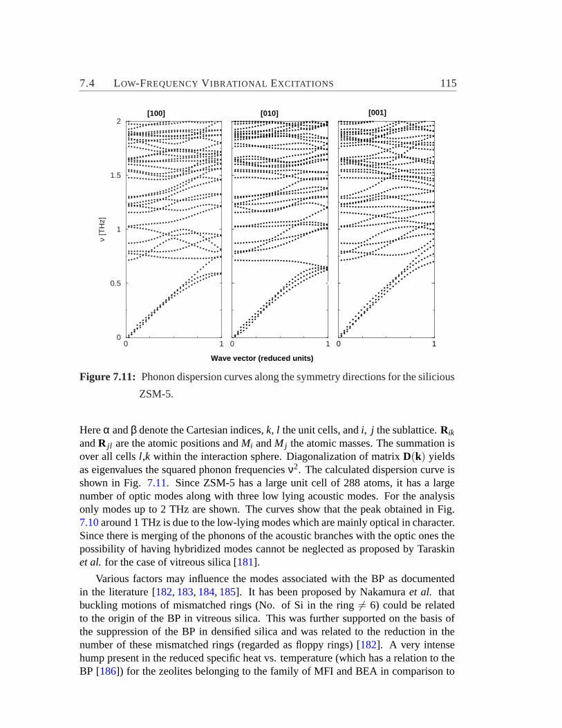
7.4 LOW-FREQUENCYV IBRATIONAL EXCITATIONS 115
0 10
0.5
1
1.5
2
ν [T
Hz]
0 10
0.5
1
1.5
2
0 10
0.5
1
1.5
2[001][100] [010]
Wave vector (reduced units)
Figure 7.11: Phonon dispersion curves along the symmetry directions for the silicious
ZSM-5.
Hereα andβ denote the Cartesian indices,k, l the unit cells, andi, j the sublattice.Rik
andR jl are the atomic positions andMi andM j the atomic masses. The summation isover all cellsl ,k within the interaction sphere. Diagonalization of matrixD(k) yieldsas eigenvalues the squared phonon frequenciesν2. The calculated dispersion curve isshown in Fig. 7.11. Since ZSM-5 has a large unit cell of 288 atoms, it has a largenumber of optic modes along with three low lying acoustic modes. For the analysisonly modes up to 2 THz are shown. The curves show that the peak obtained in Fig.7.10around 1 THz is due to the low-lying modes which are mainly optical in character.Since there is merging of the phonons of the acoustic branches with the optic ones thepossibility of having hybridized modes cannot be neglected as proposed by Taraskinet al. for the case of vitreous silica [181].
Various factors may influence the modes associated with the BP as documentedin the literature [182, 183, 184, 185]. It has been proposed by Nakamuraet al. thatbuckling motions of mismatched rings (No. of Si in the ring6= 6) could be relatedto the origin of the BP in vitreous silica. This was further supported on the basis ofthe suppression of the BP in densified silica and was related to the reduction in thenumber of these mismatched rings (regarded as floppy rings) [182]. A very intensehump present in the reduced specific heat vs. temperature (which has a relation to theBP [186]) for the zeolites belonging to the family of MFI and BEA in comparison to
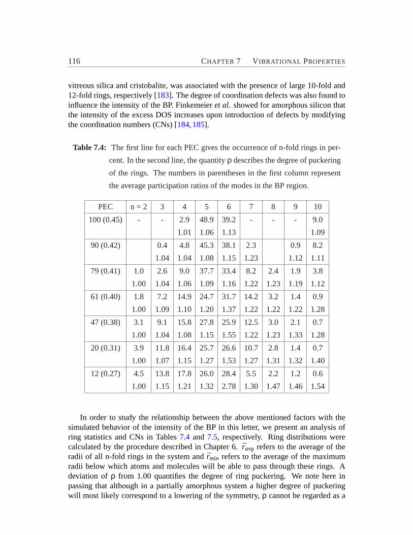
116 CHAPTER 7 VIBRATIONAL PROPERTIES
vitreous silica and cristobalite, was associated with the presence of large 10-fold and12-fold rings, respectively [183]. The degree of coordination defects was also found toinfluence the intensity of the BP. Finkemeieret al. showed for amorphous silicon thatthe intensity of the excess DOS increases upon introduction of defects by modifyingthe coordination numbers (CNs) [184,185].
Table 7.4: The first line for each PEC gives the occurrence of n-fold rings in per-
cent. In the second line, the quantityρ describes the degree of puckering
of the rings. The numbers in parentheses in the first column represent
the average participation ratios of the modes in the BP region.
PEC n = 2 3 4 5 6 7 8 9 10
100 (0.45) - - 2.9 48.9 39.2 - - - 9.0
1.01 1.06 1.13 1.09
90 (0.42) 0.4 4.8 45.3 38.1 2.3 0.9 8.2
1.04 1.04 1.08 1.15 1.23 1.12 1.11
79 (0.41) 1.0 2.6 9.0 37.7 33.4 8.2 2.4 1.9 3.8
1.00 1.04 1.06 1.09 1.16 1.22 1.23 1.19 1.12
61 (0.40) 1.8 7.2 14.9 24.7 31.7 14.2 3.2 1.4 0.9
1.00 1.09 1.10 1.20 1.37 1.22 1.22 1.22 1.28
47 (0.38) 3.1 9.1 15.8 27.8 25.9 12.5 3.0 2.1 0.7
1.00 1.04 1.08 1.15 1.55 1.22 1.23 1.33 1.28
20 (0.31) 3.9 11.8 16.4 25.7 26.6 10.7 2.8 1.4 0.7
1.00 1.07 1.15 1.27 1.53 1.27 1.31 1.32 1.40
12 (0.27) 4.5 13.8 17.8 26.0 28.4 5.5 2.2 1.2 0.6
1.00 1.15 1.21 1.32 2.78 1.30 1.47 1.46 1.54
In order to study the relationship between the above mentioned factors with thesimulated behavior of the intensity of the BP in this letter, we present an analysis ofring statistics and CNs in Tables7.4 and7.5, respectively. Ring distributions werecalculated by the procedure described in Chapter 6.ravg refers to the average of theradii of all n-fold rings in the system andrmin refers to the average of the maximumradii below which atoms and molecules will be able to pass through these rings. Adeviation ofρ from 1.00 quantifies the degree of ring puckering. We note here inpassing that although in a partially amorphous system a higher degree of puckeringwill most likely correspond to a lowering of the symmetry,ρ cannot be regarded as a
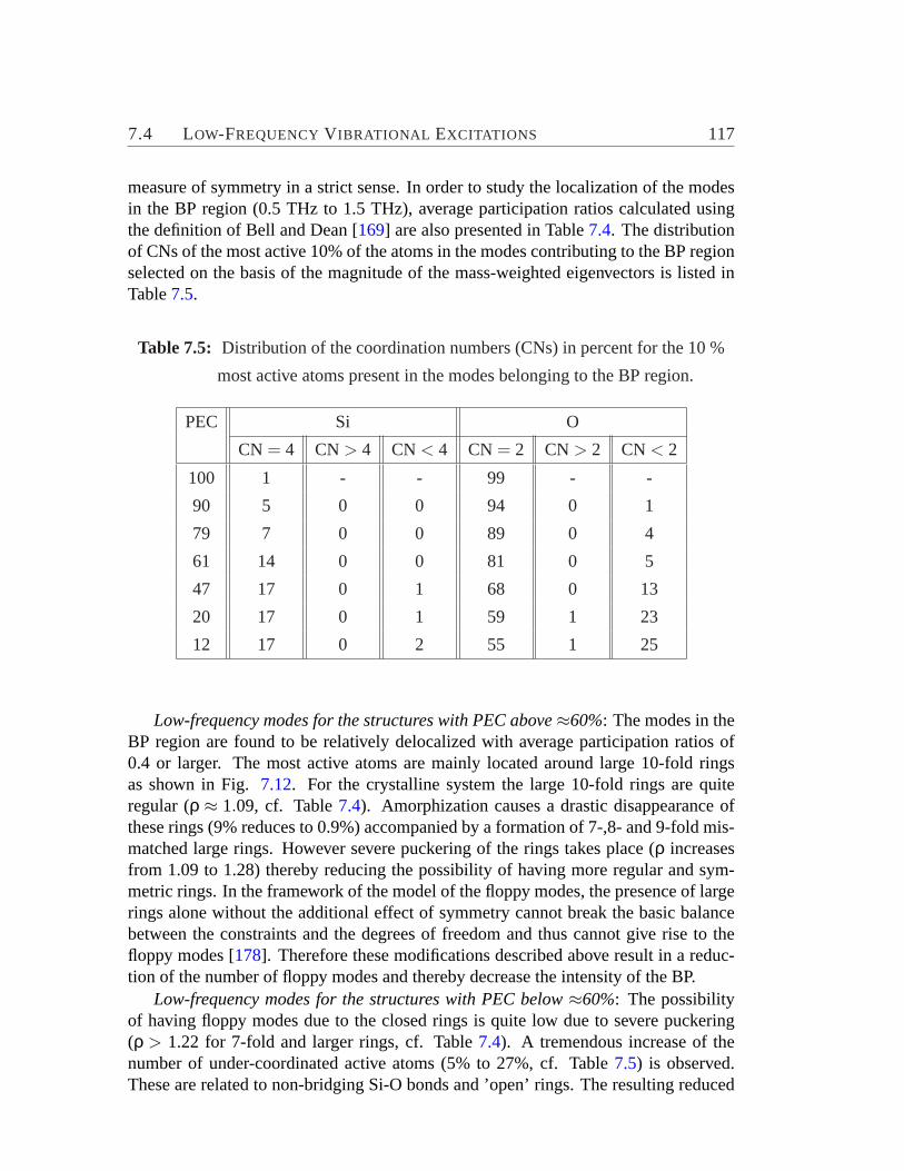
7.4 LOW-FREQUENCYV IBRATIONAL EXCITATIONS 117
measure of symmetry in a strict sense. In order to study the localization of the modesin the BP region (0.5 THz to 1.5 THz), average participation ratios calculated usingthe definition of Bell and Dean [169] are also presented in Table7.4. The distributionof CNs of the most active 10% of the atoms in the modes contributing to the BP regionselected on the basis of the magnitude of the mass-weighted eigenvectors is listed inTable7.5.
Table 7.5: Distribution of the coordination numbers (CNs) in percent for the 10 %
most active atoms present in the modes belonging to the BP region.
PEC Si O
CN = 4 CN > 4 CN < 4 CN = 2 CN > 2 CN < 2
100 1 - - 99 - -
90 5 0 0 94 0 1
79 7 0 0 89 0 4
61 14 0 0 81 0 5
47 17 0 1 68 0 13
20 17 0 1 59 1 23
12 17 0 2 55 1 25
Low-frequency modes for the structures with PEC above≈60%: The modes in theBP region are found to be relatively delocalized with average participation ratios of0.4 or larger. The most active atoms are mainly located around large 10-fold ringsas shown in Fig.7.12. For the crystalline system the large 10-fold rings are quiteregular (ρ ≈ 1.09, cf. Table7.4). Amorphization causes a drastic disappearance ofthese rings (9% reduces to 0.9%) accompanied by a formation of 7-,8- and 9-fold mis-matched large rings. However severe puckering of the rings takes place (ρ increasesfrom 1.09 to 1.28) thereby reducing the possibility of having more regular and sym-metric rings. In the framework of the model of the floppy modes, the presence of largerings alone without the additional effect of symmetry cannot break the basic balancebetween the constraints and the degrees of freedom and thus cannot give rise to thefloppy modes [178]. Therefore these modifications described above result in a reduc-tion of the number of floppy modes and thereby decrease the intensity of the BP.
Low-frequency modes for the structures with PEC below≈60%: The possibilityof having floppy modes due to the closed rings is quite low due to severe puckering(ρ > 1.22 for 7-fold and larger rings, cf. Table7.4). A tremendous increase of thenumber of under-coordinated active atoms (5% to 27%, cf. Table7.5) is observed.These are related to non-bridging Si-O bonds and ’open’ rings. The resulting reduced
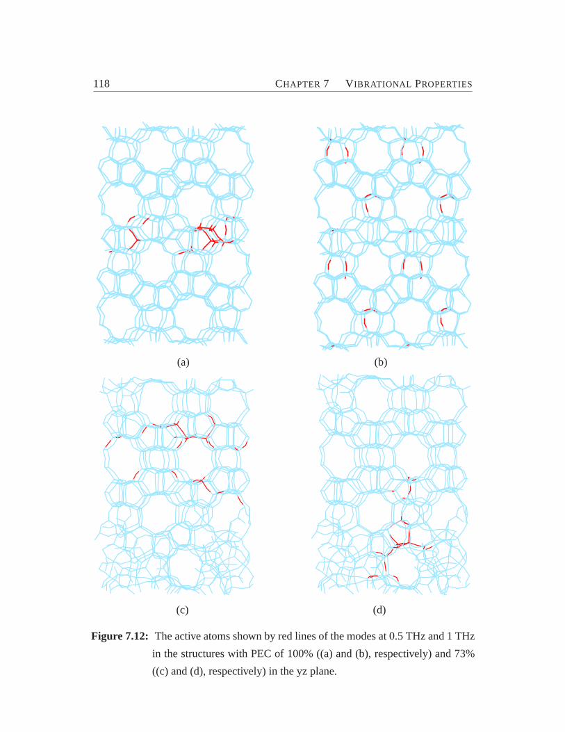
118 CHAPTER 7 VIBRATIONAL PROPERTIES
(a) (b)
(c) (d)
Figure 7.12: The active atoms shown by red lines of the modes at 0.5 THz and 1 THz
in the structures with PEC of 100% ((a) and (b), respectively) and 73%
((c) and (d), respectively) in the yz plane.
7.4 LOW-FREQUENCYV IBRATIONAL EXCITATIONS 119
number of constraints leads to an increase of the number of floppy modes. Note thatfor the structures with PEC larger than≈60% this effect is largely suppressed due tothe much lower number of active under-coordinated centers. The average participationratio decreases drastically on amorphization (from 0.40 to 0.27 for structures withPEC of 61% to 12%), with the formation of highly localized modes as shown in Fig.7.13. The increased number of these localized floppy modes associated with under-coordinated centers causes most likely the increased intensity of the BP for this rangeof PEC.
0.5 1 1.5ν [THz]
0
0.2
0.4
0.6
0.8
part
icip
atio
n ra
tio p
j
100 %47 %20 %12 %
Figure 7.13: Participation ratios of the low-frequency modes of the partially crys-
talline structures corresponding to different PEC.
Nature of the vibrational motions in low-frequency modes: We performed an anal-ysis similar to the one used by Taraskin and Elliot [166]. We projected the eigenvectorsof the SiO4 and Si-O-Si structural subunits (active subunits) containing active Si and Oatoms onto the vibrational vectors of the ideal SiO4 and Si-O-Si units with Td and C2v
symmetry, respectively. The calculated contributions of the vibrational motions exhib-ited by the active subunits are shown in Table7.6. Obviously the stretching motionsof both kinds of active subunits contribute negligibly. For the active SiO4 subunits themain contributions result from the rotational motions. However, for intermediate andlow values of PEC the bending character contributes noticeably, indicating that dis-tortions of the SiO4 subunits are associated with these low-frequency modes. Hencethe floppy modes are not in strict sense rigid unit modes in these systems. The mo-tions of the active Si-O-Si structural units involve a strong mixing of both bending androtational motions for the crystalline case (43% and 56%, respectively). Upon amor-phization the bending character decreases and the vibrational motions become mainlyrotational in nature. Since the BP occurring in the partially crystalline forms are in the

120 CHAPTER 7 VIBRATIONAL PROPERTIES
same frequency region as for the crystalline one, although with a reduced intensity asshown in Fig.7.10, we predict that the modes are mainly optic in nature.
Table 7.6: Contributions (in percent) of the vibrational motions exhibited by the
active subunits (SiO4 and Si-O-Si) as described in the text. ’S’, ’B’
and ’Rot.’ represent the stretching, bending and rotational contributions,
respectively and the superscripts denote the symmetry of the motions.
PEC SiO4 Si-O-Si
S(A1) S(F2) B(F2) B(E) Rot. S(A1) S(B1) B(A1) Rot.
100 1 1 4 1 93 0 0 43 56
90 1 1 4 2 93 1 0 40 59
79 0 0 6 3 90 1 0 37 62
61 0 0 8 4 88 0 0 29 71
47 0 0 9 6 84 0 0 27 72
20 0 0 6 5 89 0 0 20 79
12 0 0 6 4 90 0 0 16 84
Hence, we conclude that in relatively high crystalline porous structures, the de-crease in the intensity of the BP can be associated with the reduction in the numberof the floppy modes due to the decrease in the concentration of the large memberedrings and the lowering of their symmetry upon amorphization. The opposite behaviorfor relatively low crystalline structures is explained by the increased number of floppymodes due to the formation of non-bridging bonds and ’open’ rings. Although theremay exist other mechanisms which are not investigated in this thesis, floppy modes as-sociated with ’open’ rings and coordination defects have most likely a strong influenceof the intensity of the BP in partially crystalline zeolitic systems.
This part of work is published in Refs. [187,188]
Chapter 8
Relaxation Properties
Amorphous phases exhibit over an extremely broad range of time particular motionalprocesses known as relaxations [189,190,191,192,193]. Classical relaxation in glasses,sometimes also calledsecondary relaxationto distinguish it from the primary relax-ation at the glass transition, is generally believed to be well described in terms of theArrhenius-Kramers picture [194], with a relaxation timeτ given by the Arrhenius re-lation
τ = τ0exp( E
kBT
), (8.1)
whereτ0 is a macroscopic time of the order of 10−13 s, E is the energy of the barrier be-tween two energy minima of the system. The secondary orβ relaxations are envisagedas thermally activated transitions over the barriers separating the local minima in thepotential energy landscape [195,196,197], thus an insight into the topography of theinherent structures can be obtained by investigating these relaxations [167,198,199].
In contrast, the primary relaxation process orα-process, the onset of the flow pro-cess at the glass transition temperatureTg and above, seems to follow a much steeperlaw [200,201]
τ = τ0exp( A
(T−T0)
), (8.2)
whereA and T0 are constants with the dimension of temperature. This is the wellknown empirical Vogel-Fulcher-Tamman equation.
In the following sections we present a MD investigation of secondary relaxationsoccurring in our chosen model system, i.e., (partially) amorphous-forms derived fromzeolite ZSM-5. The occurrence of these relaxations might change the level of crys-tallinity and hence, it can effect the selectivity of the reactions which are dependent onthe percentage of crystallinity [28]. The dynamics show some interesting phenomenalike aging and dynamical heterogeneities at the intermediate time scales studied (1 ps
121
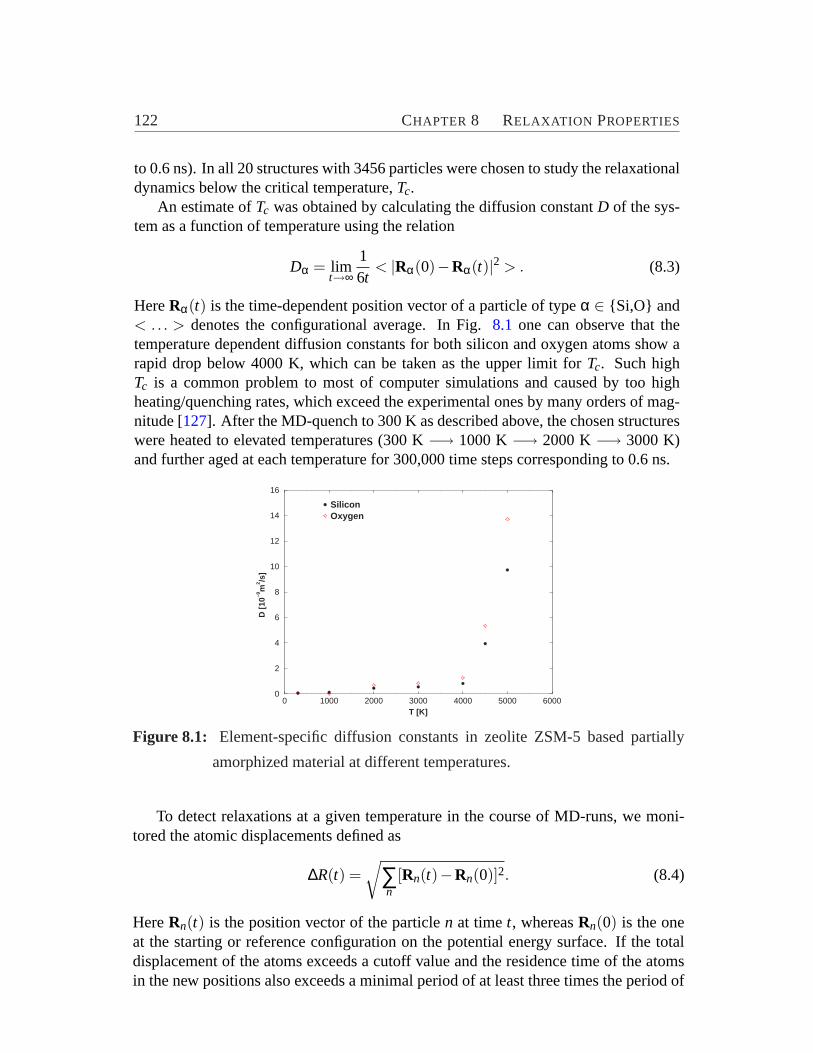
122 CHAPTER 8 RELAXATION PROPERTIES
to 0.6 ns). In all 20 structures with 3456 particles were chosen to study the relaxationaldynamics below the critical temperature,Tc.
An estimate ofTc was obtained by calculating the diffusion constantD of the sys-tem as a function of temperature using the relation
Dα = limt→∞
16t
< |Rα(0)−Rα(t)|2 > . (8.3)
HereRα(t) is the time-dependent position vector of a particle of typeα ∈ {Si,O} and< .. . > denotes the configurational average. In Fig.8.1 one can observe that thetemperature dependent diffusion constants for both silicon and oxygen atoms show arapid drop below 4000 K, which can be taken as the upper limit forTc. Such highTc is a common problem to most of computer simulations and caused by too highheating/quenching rates, which exceed the experimental ones by many orders of mag-nitude [127]. After the MD-quench to 300 K as described above, the chosen structureswere heated to elevated temperatures (300 K−→ 1000 K−→ 2000 K−→ 3000 K)and further aged at each temperature for 300,000 time steps corresponding to 0.6 ns.
0 1000 2000 3000 4000 5000 6000T [K]
0
2
4
6
8
10
12
14
16
D [
10−9
m2 /s
]
SiliconOxygen
Figure 8.1: Element-specific diffusion constants in zeolite ZSM-5 based partially
amorphized material at different temperatures.
To detect relaxations at a given temperature in the course of MD-runs, we moni-tored the atomic displacements defined as
∆R(t) =√
∑n
[Rn(t)−Rn(0)]2. (8.4)
HereRn(t) is the position vector of the particlen at timet, whereasRn(0) is the oneat the starting or reference configuration on the potential energy surface. If the totaldisplacement of the atoms exceeds a cutoff value and the residence time of the atomsin the new positions also exceeds a minimal period of at least three times the period of

8.1 TIME EVOLUTION ON THE ENERGY LANDSCAPE 123
a typical soft vibrational mode, the new positions of the particles were accepted as astarting point for the determination of a possible new minimum configuration. All thestored coordinates were then quenched toT = 0 K using a combined SDCG algorithm[132] to locate the nearest minimum configuration in the potential energy surface.In the following section we discuss on the relaxation properties of these minimumstructures during aging at the temperatures mentioned above.
8.1 Time Evolution on the Energy Landscape
Figs.8.2(a) and (b) show the time evolution of the ensemble averaged potential ener-gies and displacements per atom obtained during the aging of the systems at differenttemperatures. These averages were taken over ten configurations with a starting aver-age PEC of 60%. In general the potential energy drops during aging. After heatingthere is a subsequent leveling off of the potential energy at lower temperatures (300Kand 1000K). The largest part of the atomic-displacement immediately follows afterheating. The average displacements of the atoms is very small, i.e., less than 2% of theSi-O bond distance at 3000 K. The decrease in the average potential energy and dis-placement per atom increases with temperature as the possibility to cross large energybarriers and to visit farther away minima in potential energy landscape increases.
8.2 Structure and Mode of Relaxations
To study the localization behavior of the relaxations we calculated analogous to ourstudy of the vibrations (chapter 7), the relaxational effective mass and participationratio. The effective mass of a relaxation is defined as
Me f f = mmax(∆R0)2
|(∆R0max)2| , (8.5)
where∆R0 represents the distance between two successive minimum configurations asobtained using Eq. (8.4). |∆(R0
max)2| andmmax denote the maximal distance and mass
of the farthest jumping atom. The participation ratio is defined as,
P∆R0 =(∆R0)4
N∑n(Ri,0n −R f ,0
n )4, (8.6)
whereRi,0n andR f ,0
n denote the initial and the final position of the atomn andN repre-sents the total number of atoms. The participation ratio has the valuen/N if n atomsare equally involved in the relaxation process. If all atoms contribute equally in thejump, the resulting participation ratio will be 1.
The influence of the temperature on the jump lengths and the participation ratiosare shown in Fig.8.3. The participation ratios roughly grow linearly with the jump
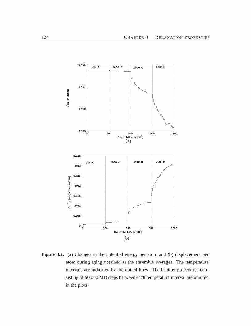
124 CHAPTER 8 RELAXATION PROPERTIES
0 300 600 900 1200No. of MD step [103
]
−17.09
−17.08
−17.07
−17.06E
0 /N [
eV/a
tom
]300 K 1000 K 2000 K 3000 K
(a)
0 300 600 900 1200No. of MD step [103]
0
0.005
0.01
0.015
0.02
0.025
0.03
0.035
∆R0 /N
[Ang
stro
em/a
tom
]
300 K 1000 K 2000 K 3000 K
(b)
Figure 8.2: (a) Changes in the potential energy per atom and (b) displacement per
atom during aging obtained as the ensemble averages. The temperature
intervals are indicated by the dotted lines. The heating procedures con-
sisting of 50,000 MD steps between each temperature interval are omitted
in the plots.
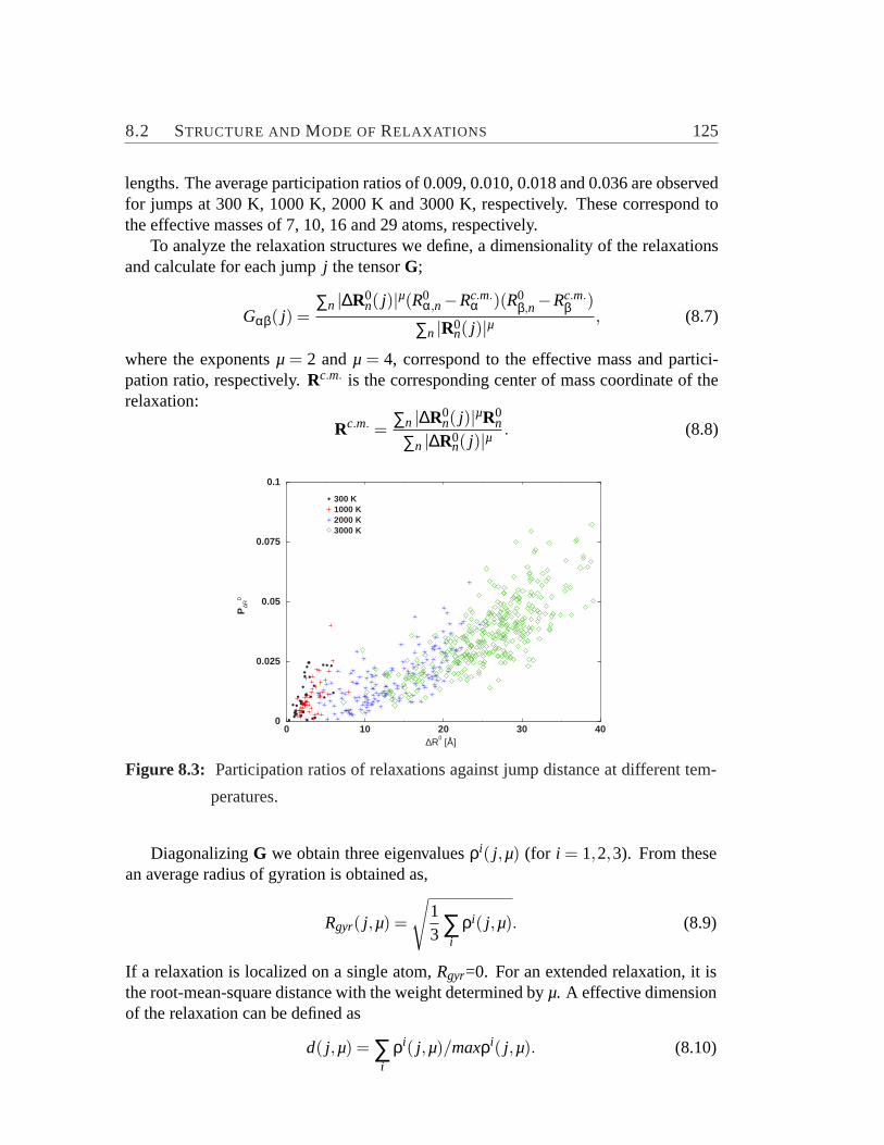
8.2 STRUCTURE AND MODE OFRELAXATIONS 125
lengths. The average participation ratios of 0.009, 0.010, 0.018 and 0.036 are observedfor jumps at 300 K, 1000 K, 2000 K and 3000 K, respectively. These correspond tothe effective masses of 7, 10, 16 and 29 atoms, respectively.
To analyze the relaxation structures we define, a dimensionality of the relaxationsand calculate for each jumpj the tensorG;
Gαβ( j) =∑n |∆R0
n( j)|µ(R0α,n−Rc.m.
α )(R0β,n−Rc.m.
β )
∑n |R0n( j)|µ , (8.7)
where the exponentsµ = 2 andµ = 4, correspond to the effective mass and partici-pation ratio, respectively.Rc.m. is the corresponding center of mass coordinate of therelaxation:
Rc.m. = ∑n |∆R0n( j)|µR0
n
∑n |∆R0n( j)|µ . (8.8)
0 10 20 30 40∆R
0 [Å]
0
0.025
0.05
0.075
0.1
P∆R
0
300 K1000 K2000 K3000 K
Figure 8.3: Participation ratios of relaxations against jump distance at different tem-
peratures.
DiagonalizingG we obtain three eigenvaluesρi( j,µ) (for i = 1,2,3). From thesean average radius of gyration is obtained as,
Rgyr( j,µ) =
√13∑
iρi( j,µ). (8.9)
If a relaxation is localized on a single atom,Rgyr=0. For an extended relaxation, it isthe root-mean-square distance with the weight determined byµ. A effective dimensionof the relaxation can be defined as
d( j,µ) = ∑i
ρi( j,µ)/maxρi( j,µ). (8.10)
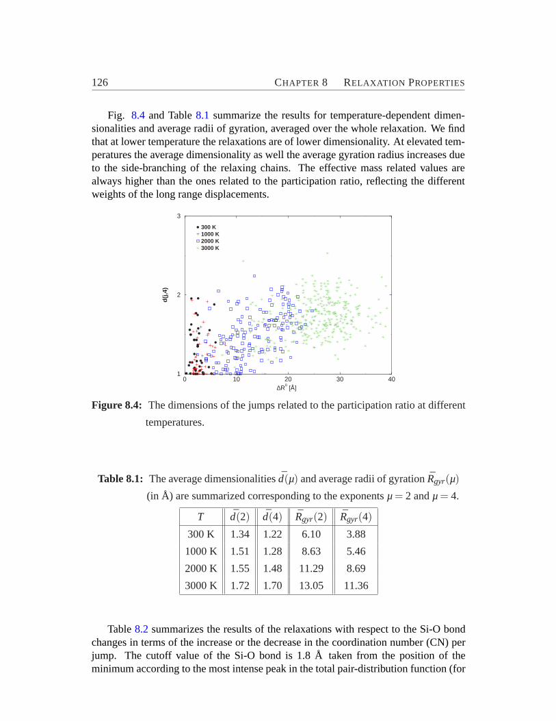
126 CHAPTER 8 RELAXATION PROPERTIES
Fig. 8.4 and Table8.1 summarize the results for temperature-dependent dimen-sionalities and average radii of gyration, averaged over the whole relaxation. We findthat at lower temperature the relaxations are of lower dimensionality. At elevated tem-peratures the average dimensionality as well the average gyration radius increases dueto the side-branching of the relaxing chains. The effective mass related values arealways higher than the ones related to the participation ratio, reflecting the differentweights of the long range displacements.
0 10 20 30 40∆R
0 [Å]
1
2
3
d(j
,4)
300 K1000 K2000 K3000 K
Figure 8.4: The dimensions of the jumps related to the participation ratio at different
temperatures.
Table 8.1: The average dimensionalitiesd(µ) and average radii of gyrationRgyr(µ)
(in Å) are summarized corresponding to the exponentsµ= 2 andµ= 4.
T d(2) d(4) Rgyr(2) Rgyr(4)
300 K 1.34 1.22 6.10 3.88
1000 K 1.51 1.28 8.63 5.46
2000 K 1.55 1.48 11.29 8.69
3000 K 1.72 1.70 13.05 11.36
Table8.2 summarizes the results of the relaxations with respect to the Si-O bondchanges in terms of the increase or the decrease in the coordination number (CN) perjump. The cutoff value of the Si-O bond is 1.8 Å taken from the position of theminimum according to the most intense peak in the total pair-distribution function (for

8.2 STRUCTURE AND MODE OFRELAXATIONS 127
details refer Fig.6.2(a)). Another possibility may be that the CN is conserved but theatoms can switch bonds during the relaxation. We denote such changes as bond switchin Table8.2. At lower temperature (1000 K and below) the relaxations are mainlydue to the small changes in the atomic positions and bond breaking occurs only in fewcases. At elevated temperatures, bond formations and dissociations occur for 3.38 % ofthe atoms. The percentage of bond switching processes seems to increase significantlyfrom 0.65% to 2.56% on elevating the temperature from 2000 K to 3000 K.
Table 8.2: Relaxation with respect to bond changes. The numbers represent the
percentage of atoms undergoing the mentioned changes per jump.
T increase in CN decrease in CN bond switch
300 K 0.04 0.04 -
1000 K 0.04 0.04 0.01
2000 K 0.24 0.23 0.65
3000 K 0.41 0.41 2.56
Table 8.3: Contributions (in percent) of the relaxations exhibited by Si-O-Si and
SiO4 subunits by the projectional analysis. ’S’, ’B’ and ’Rot.’ represent
the stretching, bending and rotational contributions, respectively and the
superscripts denote the symmetry of the motions.
T SiO4 Si-O-Si
S(A1) S(F2) B(F2) B(E) Rot. S(A1) S(B1) B(A1) Rot.
300K 1 1 11 10 77 1 0 18 81
1000K 0 0 9 14 77 0 0 17 83
2000K 1 2 11 10 76 1 1 20 78
3000K 1 3 11 9 76 2 1 21 76
In order to study the type of motions involved during the relaxations, we performedthe projections of the relaxation vectors onto the symmetry modes of the ideal Si-O-Si (C2v symmetry) and SiO4 (Td symmetry) subunits, analogous to the mode analysisfor studying the vibrational properties (cf. chapter 7). The calculated contributions ofthe motion involved in the relaxations exhibited by the subunits are shown in Table8.3. The respective motions of the oxygen and silicon atoms in the SiO4 and Si-O-Sisubunits mostly stem from rotation followed by bending. The rotational contribution of
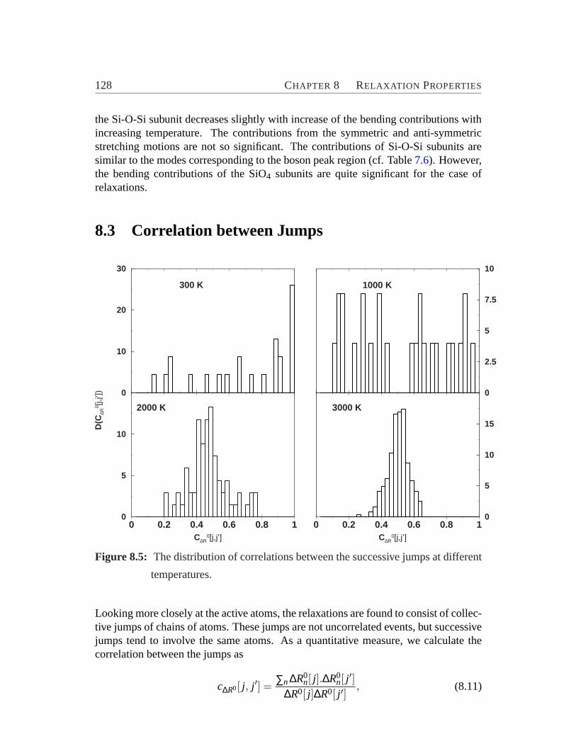
128 CHAPTER 8 RELAXATION PROPERTIES
the Si-O-Si subunit decreases slightly with increase of the bending contributions withincreasing temperature. The contributions from the symmetric and anti-symmetricstretching motions are not so significant. The contributions of Si-O-Si subunits aresimilar to the modes corresponding to the boson peak region (cf. Table7.6). However,the bending contributions of the SiO4 subunits are quite significant for the case ofrelaxations.
8.3 Correlation between Jumps
0 0.2 0.4 0.6 0.8 1C∆R
0[j,j’]
0
5
10
D(C
∆R0 [
j,j’])
2000 K
0
10
20
30
300 K
0 0.2 0.4 0.6 0.8 1C∆R
0[j,j’]
0
5
10
15
3000 K
0
2.5
5
7.5
10
1000 K
Figure 8.5: The distribution of correlations between the successive jumps at different
temperatures.
Looking more closely at the active atoms, the relaxations are found to consist of collec-tive jumps of chains of atoms. These jumps are not uncorrelated events, but successivejumps tend to involve the same atoms. As a quantitative measure, we calculate thecorrelation between the jumps as
c∆R0[ j, j ′] = ∑n∆R0n[ j].∆R0
n[ j′]
∆R0[ j]∆R0[ j ′], (8.11)

8.4 HETEROGENEITY 129
where j and j ′ denotes successive relaxations. For reversible jumps,c∆R0[ j, j ′]=1 andfor completely uncorrelated jumps one would get values of the order of 1/N.
Fig. 8.5 shows the observed distributions of all the correlation values averagedover all the relaxations. At low temperatures (300 K and 1000 K) there exists a widedistribution of the correlations. Extremely high-correlated jumps are mainly due to re-versible jumps, whereas very low-correlated ones imply that the different parts of theactive regions of the system contribute to the relaxations at different times. In contraryat high temperatures (2000 K and 3000 K), the jumps with very high and very low cor-relations become rare. The former case is due to a strong drop in the potential energyand hence, the possibility of having reversible jumps or highly correlated successivejumps are removed. The latter case is due to the aggregation of different active regionsto form large complexes and thus decreasing the possibility of jumps with very lowcorrelations.
8.4 Heterogeneity
In recent years one particular aim of intensive experimental and theoretical studies ofrelaxations in amorphous solids and liquids was to determine whether the relaxationsinvolve only groups of atoms or they are spread over the whole system [202,203,204,205]. While the first case is related to the heterogeneous scenario, the latter featuresare homogeneous ones. Various investigations showed that the system becomes ho-mogeneous at high temperatures for sufficiently long times, corresponding to theαrelaxation regime [206, 207]. In the intermediate time domain, corresponding to theβ relaxation, the heterogeneity becomes more pronounced when the system is cooleddown [150].
A detailed picture about the atomic-motions in the relaxations can be obtained byinvestigating the self part of the van Hove correlation functionGs(R, t), defined as,
Gαs (R, t) =
⟨ 1Nα
Nα
∑i=1
δ(R−|Ri(t)−Ri(0)|)⟩. (8.12)
Ri(t) is the time-dependent position vector of atomi and Ri(0) corresponds to theinitial configuration. If all the atoms have the same mobility the van Hove correlationfunction is a Gaussian one. However if atoms are trapped in cages or some are moremobile than the rest, the resulting function will be a non-Gaussian one.
In Fig. 8.6 we show the time-dependent element-specific van Hove correlationfunctions at 1000 K, 2000 K and 3000 K and at times 0.02 ns, 0.2 ns and 0.6 ns.We observe that with increasing temperature, the atoms move over larger distancesas the particles have higher diffusion constants. A striking feature occurs at 2000 K,especially for oxygen, where a formation of distinct peaks in the correlation functionhas been observed. At still higher temperature (3000 K), these peaks develop into
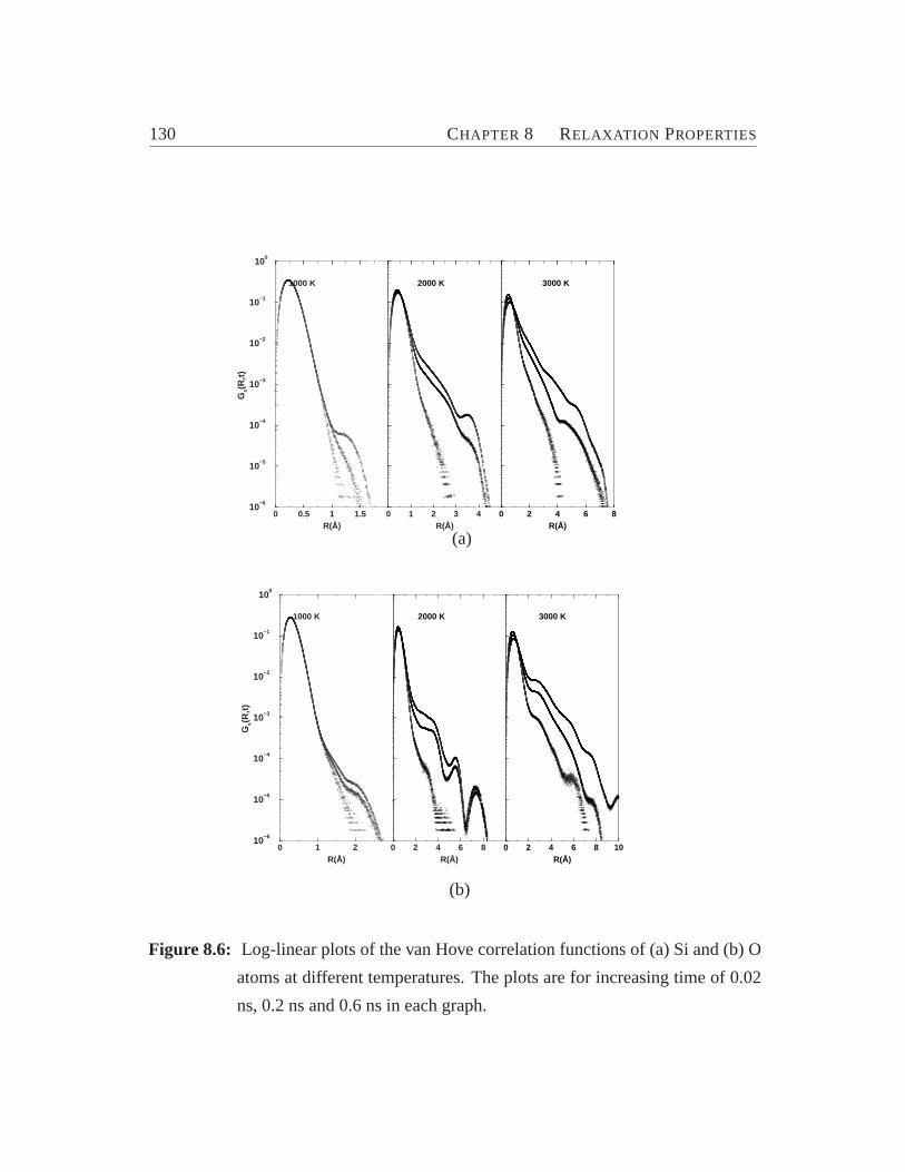
130 CHAPTER 8 RELAXATION PROPERTIES
0 0.5 1 1.5R(Å)
10−6
10−5
10−4
10−3
10−2
10−1
100
Gs(
R,t
)
1000 K
0 1 2 3 4R(Å)
10−6
10−5
10−4
10−3
10−2
10−1
100
2000 K
0 2 4 6 8R(Å)
10−6
10−5
10−4
10−3
10−2
10−1
100
3000 K
(a)
0 1 2R(Å)
10−6
10−5
10−4
10−3
10−2
10−1
100
Gs(
R,t
)
1000 K
0 2 4 6 8R(Å)
10−6
10−5
10−4
10−3
10−2
10−1
100
2000 K
0 2 4 6 8 10R(Å)
10−6
10−5
10−4
10−3
10−2
10−1
100
3000 K
(b)
Figure 8.6: Log-linear plots of the van Hove correlation functions of (a) Si and (b) O
atoms at different temperatures. The plots are for increasing time of 0.02
ns, 0.2 ns and 0.6 ns in each graph.
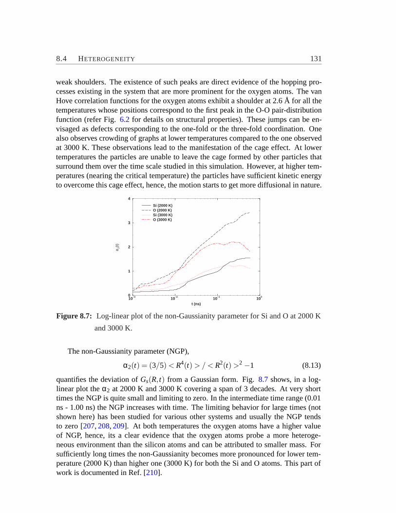
8.4 HETEROGENEITY 131
weak shoulders. The existence of such peaks are direct evidence of the hopping pro-cesses existing in the system that are more prominent for the oxygen atoms. The vanHove correlation functions for the oxygen atoms exhibit a shoulder at 2.6 Å for all thetemperatures whose positions correspond to the first peak in the O-O pair-distributionfunction (refer Fig.6.2 for details on structural properties). These jumps can be en-visaged as defects corresponding to the one-fold or the three-fold coordination. Onealso observes crowding of graphs at lower temperatures compared to the one observedat 3000 K. These observations lead to the manifestation of the cage effect. At lowertemperatures the particles are unable to leave the cage formed by other particles thatsurround them over the time scale studied in this simulation. However, at higher tem-peratures (nearing the critical temperature) the particles have sufficient kinetic energyto overcome this cage effect, hence, the motion starts to get more diffusional in nature.
10−3 10−2 10−1 100
t (ns)
0
1
2
3
4
α 2(t)
Si (2000 K)O (2000 K)Si (3000 K)O (3000 K)
Figure 8.7: Log-linear plot of the non-Gaussianity parameter for Si and O at 2000 K
and 3000 K.
The non-Gaussianity parameter (NGP),
α2(t) = (3/5) < R4(t) > / < R2(t) >2−1 (8.13)
quantifies the deviation ofGs(R, t) from a Gaussian form. Fig.8.7 shows, in a log-linear plot theα2 at 2000 K and 3000 K covering a span of 3 decades. At very shorttimes the NGP is quite small and limiting to zero. In the intermediate time range (0.01ns - 1.00 ns) the NGP increases with time. The limiting behavior for large times (notshown here) has been studied for various other systems and usually the NGP tendsto zero [207, 208, 209]. At both temperatures the oxygen atoms have a higher valueof NGP, hence, its a clear evidence that the oxygen atoms probe a more heteroge-neous environment than the silicon atoms and can be attributed to smaller mass. Forsufficiently long times the non-Gaussianity becomes more pronounced for lower tem-perature (2000 K) than higher one (3000 K) for both the Si and O atoms. This part ofwork is documented in Ref. [210].


Chapter 9
Two-Fold Rings in Silicates
Most polymorphs of silicates are formed by corner-sharing of the SiO4 tetrahedrawith differing topology of the networks. However, there also exist structures likestishovite [211] and W-silica [133] containing SiO6 octahedra and edge-sharing tetra-hedra, respectively. The edge-sharing tetrahedral structures in pure silicates are quiterare in nature. Recently, Car-Parrinello MD simulations of a dehydroxylated silicasurface showed the presence of edge-sharing tetrahedra [135]. We have also obtaineda small percentage of edge-sharing tetrahedra in (partially) amorphous structures ob-tained by MD (cf. chapter 6).
Considerable interest has been focused on the study of edge-sharing SiO4 tetrahe-dra as defective centers in vitreous silica, which act as sites of high chemical reactiv-ity [212,213,214,215]. The occurrence of these edge-sharing units makes structuresgeometrically constrained and results in an energy penalty. The lack of experimentalinsight into the stability of these unusual features makes theoretical methods impor-tant tools to investigate these strained systems. The knowledge of the energy penaltypresently rests on theoretical studies of mainly small clusters using the techniques ofquantum chemistry [216,217,218] and classical force field models based on quantumchemical reference data [157]. Such calculations neglect the effect of the condensedenvironment in which the strained part of the system actually resides. Calculationson other solids showed the importance of electron correlation to allow a meaning-ful comparison of calculated quantities like cohesive energy etc. with experimentaldata [219,220]. The most widely used approach is DFT [221,222,223]. The attrac-tiveness of this method for practical calculations results mainly from the speed withwhich the computations can be carried out. Recently, Hamann used DFT based onthe generalized gradient approximation (GGA) to extract the strained energies of two-and three- membered rings in models of a SiO2 network [221]. The calculations gavemuch smaller strain energies than previously estimated from HF calculations appliedto small hydrogen-terminated molecular models [216,217,218]. However despite thelarge success in electronic structure theory DFT has the drawback that the results arehighly dependent on the chosen functional and cannot be improved in a systematic
133

134 CHAPTER 9 TWO-FOLD RINGS IN SILICATES
way. As an alternative one can use wave-function based quantum chemicalab initiotechniques (cf. chapter 5), which are free from these flaws and provide a large arrayof methods of different accuracy and computational cost. In this approach one can im-prove the calculation systematically by enlarging the basis set and by including moreterms in the expansion of the wavefunction, however at the price of a considerablyhigher computational cost.
In the following we present HF SCF calculations and subsequent correlation calcu-lations of the energy of edge-sharing tetrahedra and provide a comparison to the usualcorner-sharing tetrahedral system. We choose W-silica andα-quartz as the model sys-tems for edge-sharing and corner-sharing silicate systems, respectively. The total andcorrelation energy per unit cell of W-silica andα-quartz were obtained using a finitecluster and an incremental approach. Various non-metallic polymeric systems havebeen studied previously using the finite-cluster approach, which yielded accurate re-sults for geometries and energies [219,224]. The incremental scheme has been usedto explore cohesive and geometrical properties of covalent solids [225, 226], semi-conductors [227, 220] and ionic solids [228, 229]. Within the incremental approach,starting from HF data obtained with a standard solid state program package as CRYS-TAL [ 118], the necessary correlation corrections to the total energy per unit cell of aperiodic system can be obtained as a sum over increments defined in terms of localizedorbitals. The correlation energy increments of well localized orbitals may be derivedfrom quantum chemical calculations on finite model systems.
Figure 9.1: Model of W-silica which is characterized by weakly interacting chains of
edge-sharing SiO4 tetrahedral units. Red and green spheres represent O
and Si atoms, respectively.

9.1 APPLIED METHODS AND TECHNICAL DETAILS 135
-4-2
02
4variation of a-b plane area in percent4.2
4.4
4.6
4.8
5
5.2
c
-879.97
-879.96
-879.95
-879.94
-879.93
-879.92
E per unit cell in a.u.
Figure 9.2: Potential energy surface plotted with respect to the variations of the area
of a-b plane, where the ratioa/b is constant and the lattice parameterc in
Å.
9.1 Applied Methods and Technical Details
W-silica as shown in Fig.9.1has a body-centered orthorhombic crystal structure withIbam space-group, characterized by chains of edge-sharing SiO4 tetrahedra. Since,these chains are interacting only by weak van der Waals forces, the geometry is mainlydetermined by the lattice parameterc in the chain direction, i.e., the Si-Si distances.We have carried out series of all-electron calculations using DFT based on the GGAof Perdew and Wang (PW91) [144,230] varyingc over a range 4.2 Å to 5.2 Å.a andbwere varied with fixeda/b ratio to change thea-b plane area by±5%. These calcula-tions were performed using a new version of the CRYSTAL code, i.e., CRYSTAL2003,which can optimize the fractional coordinates implicitly [119]. These calculations areanalogous to the ones by Hamann [221] where the Si and O ion cores were repre-sented by pseudopotentials. One can see in Fig.9.2 that the potential energy surfaceis considerably flatter with respect toa,b variations compared toc variation. This isconsistent with the fact that no significant change of energy and ring geometry couldbe obtained by optimizing thea andb parameter as shown by Hamann [221]. Cal-
136 CHAPTER 9 TWO-FOLD RINGS IN SILICATES
culations with and without chain interaction at the minima show only a small energydifference of≈ 0.005a.u. Hence one can neglect the weak inter-chain interactions andconsider only a single chain for the calculation of geometries and energies.
9.1.1 Finite-Cluster approach/A simple approach
In principle, the total energyE per [Si2O4] unit cell of a single chain of W-silica maybe obtained as the limit
E = limn→∞
E(Si2nO4n+2H4)n
, (9.1)
i.e., by performing calculations for increasingly long oligomers (OH)2(Si2O4)nH2. Inorder to reduce the finite-size effects due to the termination of the oligomers by two OHand H groups saturating the dangling bonds of .(Si2O4)n., one may consider instead
E = limn→∞
∆En
= limn→∞
[E(Si2n+2O4n+6H4)−E(Si2nO4n+2H4)], (9.2)
i.e., the energy change between the subsequent oligomers differing by a single unitcell. Therefore, identical unit cells were used as building blocks for both oligomers,i.e., the geometrical optimization was restricted only to the parameters relevant for thepolymer. Eq. (9.2) was used for computing the energy per unit cell employing HF,MP2 and CC levels of theory.
9.1.2 Incremental approach
The simple approach outlined in the previous section relies on the correlated calcu-lations for the whole finite model system, i.e., all the valence electrons have to becorrelated at a time. For larger basis sets or more complex systems (as in the caseof α-quartz) this approach may become computationally too expensive. Therefore weused an incremental approach based on localized orbitals. One of the prerequisitesfor the electron correlation treatment within the incremental approach is a reliable HFground state calculation. We performed such a calculation using the periodic HF codeCRYSTAL 98 [118]. Starting from the occupied canonical orbitals of a standard SCFcalculation localized bond orbitals are generated using a suitable criterion, e.g., theFoster-Boys localization. The correlation energy per unit cell is expanded as givenin Eq. (5.50) in Chapter 5. In order to get reliable results a size-extensive correla-tion method should be used, although non-size-extensive schemes also may provide areasonable estimate. We used MP2 and CCSD for this approach for both the systems.

9.2 STRUCTURE AND STABILITY OF TWO-FOLD RING 137
9.2 Structure and Stability of Two-Fold Ring
Calculations on both the systems, i.e., W-silica andα-quartz were performed with 6-31G** basis sets [231,232]. Usually for polar polymeric systems, calculations usingthe finite-cluster approach at the HF level may not be applicable due to the long-rangeof Coulomb interactions. Nevertheless in case of W-silica the finite-cluster approachseems to be accurate enough. Forn = 4, the HF energy per Si2O4 unit is found to be-877.6282 a.u. at the optimized geometry (cf. below). The Bloch-type function basedperiodic HF code CRYSTAL 98 uses five parameters(ITOL1 to ITOL5) to determinethe accuracy of the integral evaluation with respect to the Coulomb and exchange se-ries. For the default combination (6, 6, 6, 6, 12) the HF energy per Si2O4 unit is foundto be -877.6268 a.u. and for an even tighter threshold (10, 10, 10, 12, 26) a value of-877.6278 a.u. in excellent agreement with the finite-cluster value is obtained. For theHF calculations on the infinite system, using CRYSTAL, the most diffusesp Gaus-sian exponents of the original basis sets had to be increased due to linear dependencyproblems. This led to exponents of 0.28 for oxygen (original 0.27) and 0.21 for sili-con (original0.0778). We want to mention that the energy obtained using CRYSTAL,shows a drastic dependence on thed Gaussian exponents. For the optimized geom-etry and the tighter threshold the HF energy per Si2O4 unit is found to be -877.6513a.u. with optimizedd exponents of 0.48 for oxygen and 0.72 for silicon. However forthe correlated calculations and for the comparison withα-quartz, we used the originalbasis set as a lower value of the total energy per unit cell is obtained.
The correlation energy was calculated by subtracting from the MP2, CCSD andCCSD(T) values the corresponding HF energy/ cell. In this manner we ensured thatno spurious contributions to the correlation energy arose due to the use of two differ-ent basis sets. The cohesive energies were obtained by subtracting the correspondingenergies of the free ground state atoms from the energy per unit cell. These calcula-tions were performed using the MOLPRO molecular orbitalab initio program pack-age [139,140,233]. The energy per unit cell and the cohesive energy converge rapidlywith respect to the cluster size (cf. Fig.9.3). One finds∆E4−∆E3 ≈ 10−5 a.u. (seeEq. (9.2) for definition of∆En). An all-electron CCSD(T) (CCSD with a perturbativecontribution of triples) approach could not be used to compute∆E4 due to the largesystem size. The optimized geometry reported in Fig.9.4(a) and (b) and in Table9.1was obtained by performing in turn several total energy calculations for various val-ues of each geometric parameter and fitting the results by a least-squares procedureto polynomials of suitable degrees. The computed lattice parameterc of 4.75 Å isin good agreement with the experimental value e of 4.72 Å. However, the Si-O bondlength of 1.844 Å determined in Ref. [133] appears to be un-physically large. Thisbond length is even larger that those of three-fold coordinated O in stishovite [234] aswas pointed out also in other theoretical studies [216,221]. Generally, our MP2, CCSDand CCSD(T) structural values agree with those of a previous gradient-corrected DFTstudy within 0.02 Å and 1◦.
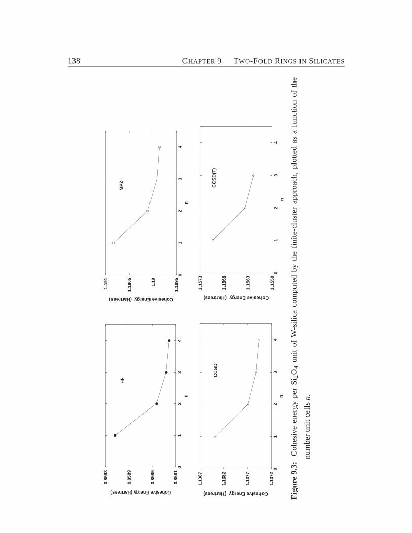
138 CHAPTER 9 TWO-FOLD RINGS IN SILICATES
01
23
4n
0.85
81
0.85
85
0.85
89
0.85
93
Cohesive Energy (Hartrees)
HF
01
23
4n
1.18
95
1.19
1.19
05
1.19
1
Cohesive Energy (Hartrees)
MP
2
01
23
4n
1.13
72
1.13
77
1.13
82
1.13
87
Cohesive Energy (Hartrees)
CC
SD
01
23
4n
1.15
58
1.15
63
1.15
68
1.15
73
Cohesive Energy (Hartrees)
CC
SD
(T)
Fig
ure
9.3:
Coh
esiv
een
ergy
per
Si
2O4
unit
ofW
-sili
caco
mpu
ted
byth
efin
ite-c
lust
erap
proa
ch,
plot
ted
asa
func
tion
ofth
e
num
ber
unit
cells
n.

9.2 STRUCTURE AND STABILITY OF TWO-FOLD RING 139
Table 9.1: Geometries of two-membered rings in W-silica.
Method c Si-O Si-O-Si O-Si-O
(Å) (Å) (◦) (◦)
CRYSTAL SCF 4.680 1.643 90.86 89.13
Finite cluster SCF 4.717 1.650 91.28 88.72
MP2 4.744 1.683 89.62 90.38
CCSD 4.744 1.676 90.09 89.91
CCSD(T) 4.745 1.680 89.81 90.19
GGAa 4.757 1.678 90.3 89.7
Expt.b 4.720 1.844 79.6 100.4a Reference [221].b Reference [133].
In order to perform a comparison of the stability of W-silica with respect toα-quartz, we performed correlated calculations for both systems on the same footing,i.e., by using the incremental approach truncated at the same level of correlation incre-ments. The experimental geometry [235] was used forα-quartz, whereas the optimizedgeometry at the CCSD level was used for W-silica (cf. above).
The HF ground state calculations were done using the CRYSTAL code. In orderto overcome the convergence problems due to too diffuse exponents and the resultingnear-linear dependencies we optimized the exponents of the most diffusespGaussiansof a 6-31G** basis set also forα-quartz as performed in Ref. [236]. For O and Sivalues of 0.28 and 0.21, respectively, were obtained. The exponents of the singledshell of O and Si were optimized to be 0.45 and 0.72 respectively. These d exponentsled to a lower total HF energy compared the to the original basis sets.
The exact equation for the infinite system, i.e., Eq. (5.50) in chapter 5 is of littleuse in practice. However, since electron correlation is a local phenomenon one mayderiveEcorr from a finite model system. Thereby changing the infinite sums in Eq.(5.50) to finite sums up to a maximum order of increments given by the number ofbondsn in the finite system. It has been shown by previous calculations that usuallythere is a rapid convergence of the many-body expansion with respect to the numberof atoms included and the integration error decreases withr−3 [220,237]. Therefore,we restricted the expansion of the correlation energy per unit cell to one- and two-body increments, and included the interaction between up to second-nearest neighborunit cells. The resulting finite clusters as shown in Fig.9.5 (a) and (b ), contain30 and 57 atoms with dangling bonds saturated by hydrogens for W-silica andα-

140 CHAPTER 9 TWO-FOLD RINGS IN SILICATES
quartz, respectively. We performed standard SCF calculations on the clusters in C1
symmetry and localized the bonds according to the Foster-Boys criterion [115] withinthe occupied valence space. Following the procedure described above we calculatedthe correlation energy increments at the MP2 and CCSD level using the MOLPROmolecular orbitalab initio program package [139,140,233]. Computed increments tothe correlation energy are summarized in Table9.2. It is interesting to note that forα-quartz the two-body increments amount to 69% and 65 % of the correlation energycomputed by the MP2 and CCSD methods, respectively.
0 1 2 3 4n
4.71
4.72
4.73
4.74
4.75
Lat
tice
par
amte
r c
(Å)
0 1 2 3 4n
1.64
1.65
1.66
1.67
1.68
1.69
Si−
O (
Å)
(a) (b)
Figure 9.4: (a) Lattice parameterc and (b) Si-O distance of W-silica computed using
the finite-cluster approach, plotted as a function of the number unit cellsn
(filled circles, squares, crosses and diamonds represent HF, MP2, CCSD
and CCSD(T) results, respectively).
The correlation contributions to the cohesive energies forα-quartz were obtainedas Ecorr
coh = Ecorrsolid−∑i E
corratom,i per SiO2 unit. The results are shown in Table9.3 for
different theoretical methods. For the best method, i.e., CCSD, we obtain 88% of theexperimental cohesive energy, which amounts to≈57% of the ”experimental” cor-relation contribution to the cohesive energies (defined as the difference between theexperimental cohesive energy and the SCF value). DFT using the local density ap-proximation (LDA) overestimates the cohesive energy by 18%.

9.2 STRUCTURE AND STABILITY OF TWO-FOLD RING 141
(a)
(b)
Figure 9.5: Finite clusters of 30 and 57 atoms of (a) a chain of W-silica and (b)α-
quartz, respectively, which are used for the incremental approach. The
reference cell is represented by red-colored spheres and the environment
by light ones. Here the small-, medium- and large-sized spheres represent
H, O and Si atoms, respectively.
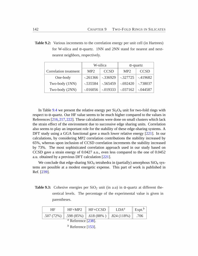
142 CHAPTER 9 TWO-FOLD RINGS IN SILICATES
Table 9.2: Various increments to the correlation energy per unit cell (in Hartrees)
for W-silica andα-quartz. 1NN and 2NN stand for nearest and next-
nearest neighbors, respectively.
W-silica α-quartz
Correlation treatment MP2 CCSD MP2 CCSD
One-body -.261366 -.336929 -.327725 -.419682
Two-body (1NN) -.535584 -.565459 -.692420 -.738037
Two-body (2NN) -.016056 -.019333 -.037162 -.044587
In Table9.4 we present the relative energy per Si2O4 unit for two-fold rings withrespect toα-quartz. Our HF value seems to be much higher compared to the values inReferences [216,217,222]. These calculations were done on small clusters which lackthe strain effect of the environment due to successive edge sharing units. Correlationalso seems to play an important role for the stability of these edge-sharing systems. ADFT study using a GGA functional gave a much lower relative energy [221]. In ourcalculations, by considering MP2 correlation contributions the stability increased by65%, whereas upon inclusion of CCSD correlation increments the stability increasedby 73%. The most sophisticated correlation approach used in our study based onCCSD gave a strain energy of 0.0427 a.u., even less compared to the one of 0.0452a.u. obtained by a previous DFT calculation [221].
We conclude that edge-sharing SiO4 tetrahedra in (partially) amorphous SiO4 sys-tems are possible at a modest energetic expense. This part of work is published inRef. [239].
Table 9.3: Cohesive energies per SiO2 unit (in a.u) inα-quartz at different the-
oretical levels. The percentage of the experimental value is given in
parentheses.
HF HF+MP2 HF+CCSD LDAa Expt.b
.507 (72%) .598 (85%) .618 (88% ) .824 (118%) .706a Reference [238].b Reference [153].
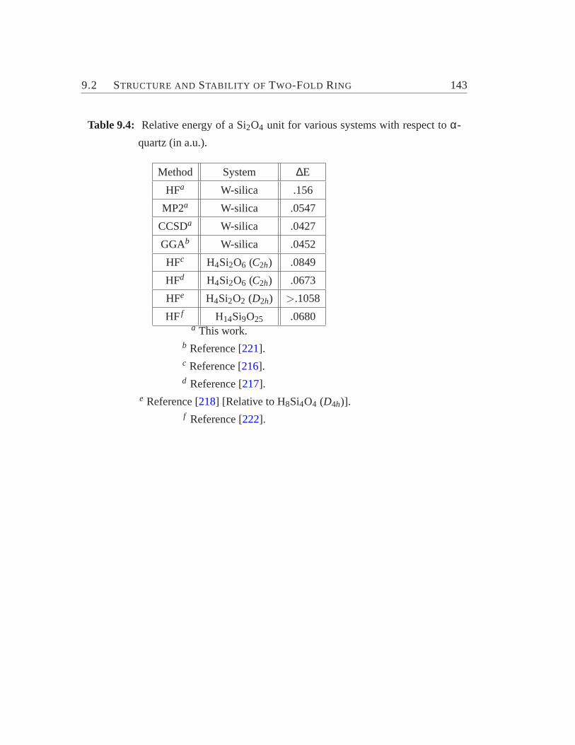
9.2 STRUCTURE AND STABILITY OF TWO-FOLD RING 143
Table 9.4: Relative energy of a Si2O4 unit for various systems with respect toα-
quartz (in a.u.).
Method System ∆E
HFa W-silica .156
MP2a W-silica .0547
CCSDa W-silica .0427
GGAb W-silica .0452
HFc H4Si2O6 (C2h) .0849
HFd H4Si2O6 (C2h) .0673
HFe H4Si2O2 (D2h) >.1058
HFf H14Si9O25 .0680a This work.
b Reference [221].c Reference [216].d Reference [217].
e Reference [218] [Relative to H8Si4O4 (D4h)].f Reference [222].

Chapter 10
Summary and Outlook
In this thesis we present an investigation of static and dynamic properties of zeoliteZSM-5-based (partially) amorphous materials. The partially amorphized structureswere obtained by quenching configurations, which were generated by heating theZSM-5 crystalline structure using MD. Our simulations gave a detailed account ofmany significant structural properties at the microscopic level which explain the modi-fied properties and applications of these low crystalline and amorphous materials. Thesimulations showed that the elementary building blocks are distorted SiO4 tetrahedrawhich are mainly connected by corner sharing. A small percentage of edge-sharedtetrahedra are also present in the simulated structures. Two-body structural correlationwas analyzed by pair-distribution functions and showed the average bond distance be-tween Si and O atoms to be about 1.62 Å. Si-Si and O-O distances correspond to 3.19Å and 2.61 Å, respectively. Three-body structural correlation was analyzed by bondangle distributions and supports the presence of mainly corner sharing tetrahedra inthe network along with a small percentage of edge-sharing ones. The extent of amor-phization was quantified by the parameter "percentage of energy crystallinity". Crucialproperties like coordination number distribution, effective internal surface area, ringsize distribution and effective pore size are found to be a functional of the extent ofamorphization. Amorphization leads to a collapse of the framework which reducesfor large species the porosity of the system and brings about a closure of large-sizedrings and channels. Whereas for larger species the effective internal surface is reducedby this process, it is increased for smaller species, probably due to the increase of theamount of under-coordinated atoms and the generation of smaller rings from largerones. Hence, it can effect properties like ion exchange and steric effects on reactions.In the amorphous phase 5-fold and 6-folds rings contribute most to the ring distribu-tion followed by 4-fold, 3-fold and 7-fold rings, however, due to irregular ring shapethe pores provided by 5-fold and especially 6-fold rings appear to be relatively small.
Vibrational densities of states were calculated by Fourier transformation of thevelocity-autocorrelation function and by the diagonalization of the dynamic matrix.The element-specific contributions show that the oxygen atoms participate more signif-
145
146 CHAPTER 10 SUMMARY AND OUTLOOK
icantly than the silicon atoms, however the contributions of the silicon atoms becomequite remarkable for the peak obtained near 24 THz. By means of the eigenmode anal-ysis it was shown that in general both silicon and oxygen atoms exhibit motions whichare perpendicular to the Si-O bonds. However oxygen atoms have also significant con-tributions for their motions parallel to the bonds. The contribution of the individualmodes to the specific heat has been analyzed and the plot ofCV/T3 with respect toTshows a maximum around 15 K.
The vibrational analysis was done in order to get an insight into the nature of vibra-tional modes, the degree of mode localization and the phase relation. We found that thelocalized modes are centered in the high-frequency region whereas the quasi-localizedstates are in the low-frequency region. The phonons in the low-frequency region aremainly acoustic in character whereas those of the high-frequency region are optic-like. Projection of the eigenmodes onto the vibrational symmetric vectors of Si-O-Siand SiO4 structural subunits suggests that for both structural subunits the asymmetricstretching motions dominantly contribute to the high-frequency region. The symmet-ric stretching motions of Si-O-Si subunits contribute mostly for the peak at 24 THz inthe mid-frequency region and for the peaks between 30 THz and 40 THz in the high-frequency region for the SiO4 subunits. The rotational and bending motions mainlycontribute for the low- and mid-frequency region. Analysis of the dependence of thevibrational DOS with respect to the degree of amorphization reveals that besides anoverall smoothening of DOS the high-frequency modes are more drastically affectedcompared to the low-frequency ones.
Analysis of the low-frequency excitations show that for higher crystallinity the in-tensity of the boson peak decreases upon amorphization, whereas the opposite behavioris observed for forms with lower crystallinity. The former effect is associated with adecrease of the concentration of 10-fold rings and a general lowering of symmetry bypuckering of large rings. The latter behavior is related to an increasing participation ofunder-coordinated centers in the relevant low-frequency motions. Both observationscan be explained in the framework of Maxwell counting of floppy modes. The modesassociated with the boson peak for these materials are found to be mainly optic innature.
The investigation of relaxational properties were restricted to the secondary pro-cesses occurring at the temperatures corresponding to 300 K, 1000 K, 2000 K and3000 K. At higher temperatures (2000 K and 3000 K), the configurations show a sharpdrop in the potential energies during aging and reflecting the possibility to visit far-ther away minima increases. At low temperatures (300 K and 1000 K), the relaxationsare mainly due to the small changes in the positions of the atoms. Bond creationsand annihilations become significant at higher temperatures (2000 K and 3000 K).The localization of the relaxations was studied using participation ratios and effec-tive masses. We found that participation ratios and jump lengths increase with theincreasing temperatures. The structure of the relaxation was quantified by the dimen-sionality of the jumps. At low temperatures the relaxations consist of chains of atomsthat are mainly one dimensional. The dimensionality of the jumps increases with the
147
temperature due to side-branching of the chains. There exists a wide distribution ofcorrelations between successive jumps at low temperatures. On increasing the temper-ature we found very high and very low correlated jumps becoming rare. The formerfact is due the sharp drop in the potential energy occurring during relaxations makingreversible jumps to become rare events. The latter is due to the aggregations of variousactive regions to form large complexes. Analysis of the heterogeneity in the relaxationsoccurring in these systems was performed by the van Hove correlation function andthe non-Gaussian parameter. The van-Hove correlation function specially for the Oatoms exhibits peaks, which are characteristic for the hopping processes. The analysisof non-Gaussianity parameters shows that the oxygen atoms probe a more heteroge-neous environment than the silicon atoms and probably attributed to the smaller massof oxygen atoms. For a longer time scale at low temperature (2000 K) the dynamicsbecomes more heterogeneous than at the higher one (3000 K). Caging effects are alsofound to be more prominent at lower temperatures.
We have performed a comparative study on periodic W-silica andα-quartz basedon correlatedab initio electronic structure calculations. The former compound is con-sidered as a model system for edge-sharing SiO4 tetrahedra silicates and the latter forcorner-sharing ones. Periodic HF theory was used to obtain the mean-field results. Thefinite-cluster and the incremental approach were used to determine correlation effectsin W-silica andα-quartz. For the finite-cluster approach, the geometry as well as theenergy per unit cell seem to converge rapidly. Our optimized geometry supports theclaim of a previous DFT study that the experimentally available Si-O distance is ab-normally large and might be incorrect. Forα-quartz we have obtained at the CCSDlevel around 88% of the experimental cohesive energy using a 6-31G** basis set. Theremaining error may be partly due to the lack of higher polarization functions in ourone-particle basis set as well as the absence of triple excitations.
Our results and those available from literature predict the strain energy associatedwith the two-fold rings to depend highly on the chosen model system as well as onthe method. Correlation contributions seem to play an important role for the relativestability of the edge-sharing units with respect to corner-sharing ones. HF calculationsdone solely on the infinite W-silica system gave a strain energy of 0.156 a.u. muchhigher than the relaxed finite-cluster calculations. Correlation contributions reduce thisresult by about a factor of three. The most sophisticated method, i.e., CCSD, gave astrain energy of 0.0427 a.u, even slightly lower than the value of 0.0452 a.u. obtainedby a previous DFT calculation. We conclude that edge-sharing SiO4 tetrahedra in(partially) amorphous SiO4 systems are possible at a modest energetic expense.
Since the success of MD depend on applied potential it will be worth to re-investigatethese properties using other potentials. The available potentials for pure silicate sys-tems are that of Vashishtaet al [165], Oumi et al [240], etc. An even deeper insightinto catalytic properties of real system can be obtained by using H-ZSM-5 for the sim-ulation. Recently, ZSM-5 based materials with XRD crystallinity levels as low as 2%exhibited superior catalytic performance in skeletal isomerization of linear butenes toiso-butenes [28]. This was ascribed to the decrease in the extend of the alkene inter-
148 CHAPTER 10 SUMMARY AND OUTLOOK
conversion and H-transfer reactions (reduced acidity) occurring as a consequence ofdecreased zeolitic pore-length. Zeolite ZSM-5 has 12 distinct site for substitution ofSi by Al. There exist numerous theoretical studies in order to determine the most fa-vorable position of Al in crystalline ZSM-5 [241,242,243]. The model of crystallineH-ZSM-5 can be build from these information. In order to model H-ZSM-5 and itsderived system the pair-potential of Krameret al [125] can be used. The method usedin this thesis can be used to generate the (partially) amorphous structures correspond-ing to different extent of amorphization. Further the active site containing Al centerscan be cut out with a few layers of environment and the geometry can be allowed torelax within the combined quantum mechanics and molecular mechanics (QM/MM)approach [244,245]. Brønsted acidities of the active sites can be studied which signif-icantly influence the occurrence of the above mentioned reaction.
Finally, the results presented in this thesis are mainly predictions using theoreticalmodel, it will be dream-coming true to see that these are confirmed by experiments infuture.

Bibliography
[1] S. R. Elliott,Physics of amorphous materials, Longman, London (1983).
[2] A. Feltz,Amorphous Inorganic Materials and Glasses, VCH Weinheim (1993).
[3] H. Salmang,Die Glasfabrikation, Springer-Verlag, Berlin (1957).
[4] J. J. Kitaigorodsky,Technologie des Glases, Verlag Technik, Berlin (1959).
[5] P. T. Sarjeant, R. Roy,J. Amer. Ceram. Soc., 52, 344 (1969).
[6] H. Dislich, J. Non-Cryst. Solids, 57, 371 (1983).
[7] R. C. Haushalter, C. M. O’Connor, J. P. Haushalter, A. M. Umarji, G. K. Shenoy,Angew. Chem., 96, 147 (1984).
[8] J. Tauc, A. Abraham, R. Zallen, M. Slade,J. Non-Cryst. Solids, 4, 279 (1970).
[9] A. Feltz, C. Kaps,Thin Solid Films, 70, 117 (1980).
[10] P. R. Stuart,Vacuum, 19, 507 (1969).
[11] F. K. McTaggart,Plasma Chemistry in Electrical Discharges, Elsevier, New York(1967).
[12] R. H. Doremus,Proc. 11th Int. Congr. GlassPrague,1, 263 (1977).
[13] R. Schrader, W. Dusdorf,Kristall und Technik, 1, 59 (1966).
[14] P. S. De Carli, J. C. Jamieson,J. Chem. Phys., 31, 1657 (1959).
[15] W. Primak,Phys. Rev., 110, 1240 (1958).
[16] A. F. Cronstedt,Akad. Handl. Stockholm, 18, 120 (1756).
[17] R. M. Barrer,Proc. Roy. Soc.(1938).
[18] R. M. Barrer, P. J. Denny,J. Chem. Soc., 971 (1961).
149
150 BIBLIOGRAPHY
[19] C. Kosanovic, A. Cizmek, B. Subotic, I. Smit, M. Stubicar, A. Tonejc,Zeolites,15, 51 (1995).
[20] C. Kosanovic, B. Subotic,Microporous Mater., 12, 261 (1997).
[21] R. A. Secco, Y. Huang,J. Phys. Chem. Solids, 60, 999 (1999)
[22] C. Kosanovic, B. Subotic, I. Smit,Thermochim. Acta, 317, 25 (1998).
[23] S. X. Wang, L. M. Wang, R. C. Ewing,J. Nucl. Mater., 278, 233 (2000).
[24] B. X. Gu, L. M. Wang, R. C. Ewing,J. Nucl. Mater., 278, 64 (2000).
[25] C. P. Nicolaides, N. P. Sincadu, M. S. Scurrell,Catal. Today, 17, 429 (2002).
[26] P. B. Venuto,Microporous Mater., 2, 297 (1994).
[27] G. H. Hutchings, C. P. Nicolaides, M. S. Scurrell,Catal. Today, 15, 23 (1992).
[28] C. P. Nicolaides,Appl. Catal. A, 185, 211 (1999).
[29] M. S. Scurrell,Appl. Catal., 4189 (1988).
[30] D. Seddon,Catal. Today, 6, 351 (1990).
[31] J. A. Biscardi, E. Iglesia,J. Catal., 182, 117 (1999).
[32] J. C. Tully,Classical and Quantum Dynamics in Condensed Phase Simulations,edited by B. J. Berne, G. Cicotti and D. F. Coker, World Scientific, Singapore(1998).
[33] J. C. Tully,Faraday Discuss., 110, 407 (1998).
[34] J. C. Burant, J. C. Tully,J. Chem. Phys., 112, 6097 (2000).
[35] A. Messiah,Quantum Mechanics, North-Holland Publishing Company, Amster-dam (1964).
[36] H. Goldstein,Classical Mechanics, Aula-Verlag, Wiesbaden (1987).
[37] G. C. Schatz,Rev. Mod. Phys., 61, 669 (1989).
[38] J. C. Greer, R. Ahlrichs and I. V. Hertel,Z. Phys. D, 18, 413 (1991).
[39] M. P. Allen, D. J. Tildesly,Computer Simulation of Liquids, Clarendon Press,Oxford (1990).
[40] C. G. Gray, K. E. Gubbins,Theory of Molecular Fluids Vol. 1, Clarendon Press,Oxford (1984).
BIBLIOGRAPHY 151
[41] D. Marx, J. Hutter,Modern Methods and Algorithms of Quantum Chemistry, NICSeries, Vol. 1 (2000).
[42] M. E. Tuckerman,Quantum Simulations of Complex Many-Body Systems: FromTheory to Algorithms, NIC Series, Vol. 10 (2002).
[43] M. Griebel, S. Knapek, G. Zumbusch, A. Caglar,Numerische Simulation in derMoleküldynamik, Springer-Verlag Berlin, Heidelberg (2004).
[44] D. C. Rapaport,The Art of Molecular Dynamics Simulation, Cambridge Univer-sity Press, Cambridge (1995).
[45] J. M. Haile,Molecular Dynamics Simulation, Wiley (1992).
[46] A. R. Leach,Molecular Modelling: Principles and Application, Pearson Educa-tion Limited, (2001).
[47] D. Frenkel, B. Smit,Understanding Molecular Simulation: From Algorithms toApplications, Academic Press, California (2002).
[48] W. Cui, F. Li, N. L. Allinger,J. Amer. Chem. Soc., 115, 2943 (1993).
[49] N. Nevins, J. H. Lii, N. L. Allinger,J. Comp. Chem., 17, 695 (1996).
[50] S. L. Mayo, B. D. Olafson, W. A. Goddard,J. Phys. Chem., 94, 8897 (1990).
[51] M. J. Bearpark, M. A. Robb, F. Bernardi, M. Olivucci,Chem. Phys. Lett., 217,513 (1994).
[52] T. Cleveland, C. R. Landis,J. Amer. Chem. Soc., 118, 6020 (1996).
[53] A. K. Rappé, C. J. Casewit, K. S. Colwell, W. A. Goddard, W. M. Skiff,J. Amer.Chem. Soc., 114, 10024 (1992).
[54] Z. W. Peng, C. S. Ewig, M. -J. Hwang, M. Waldmann, A. T. Hagler,J. Phys.Chem., 101, 7243 (1997).
[55] W. D. Cornell, P. Cieplak, C. I. Bayly, I. R. Gould, K. M. Merz, D. M. Ferguson,D. C. Spellmeyer, T. Fox, J. W. Caldwell, P. A. Kollman,J. Amer. Chem. Soc.,117, 5179 (1995).
[56] A. D. Mackerell, J. Wiorkiewiczkuczera, M. Karplus,J. Amer. Chem. Soc., 117,11946 (1995).
[57] W. L. Jorgensen, D. S. Maxwell, J. Tiradorives,J. Amer. Chem. Soc., 118, 11225(1996).
[58] T. A. Halgren,J. Comp. Chem., 17, 490 (1996).

152 BIBLIOGRAPHY
[59] J. J. Nicolas, K. E. Gubbins, W. B. Streett, D. J. Tildesly,Mol. Phys., 37, 1429(1979).
[60] P. Ewald,Ann. Phys., 64, 253 (1921).
[61] S. W. de Leeuw, J. W. Perram, E. R. Smith,Proc. R. Soc. London, A373,27(1980).
[62] S. W. de Leeuw, J. W. Perram, E. R. Smith,Proc. R. Soc. London, A373,57(1980).
[63] P. Gibbon, G. Sutmann,Quantum Simulations of Complex Many-Body Systems:From Theory to Algorithms, NIC Series, Vol. 10 (2002).
[64] D. M. Heyes,J. Chem. Phys., 74, 1924 (1981).
[65] J. W. Perram, H. G. Petersen, S. W. de Leeuw,Mol. Phys., 65, 875 (1988).
[66] D. J. Evans, W. G. Hoover, B. H. Failor, B. Moran and A. J. C. Ladd,Phys. Rev.A, 28, 1016 (1983).
[67] H. C. Andersen,J. Chem. Phys., 72, 2384, (1980).
[68] S. Nosé,J. Chem. Phys., 81, 511, (1984).
[69] M. Parrinello, A. Rahman,Phys. Rev. Lett.,45, 1196, (1980).
[70] M. Parrinello, A. Rahman,J. Appl. Phys., 52, 7182, (1981).
[71] M. Parrinello, A. Rahman,J. Chem. Phys., 76, 2662, (1982).
[72] C. A. Floudas, P. M. Pardalos,Recent Advances in Global Optimization, Prince-ton University Press, Princeton, NJ (1991).
[73] A. R. Leach,Reviews in Computational ChemistryVol-2, VCH publishers, NewYork (1991).
[74] L. Piela, J. Kostrowicki, H. A. Scheraga,J. Phys. Chem., 93, 3339, (1989).
[75] E. O. Purisima, H. A. Scheraga,Proc. Natl. Acad. Sci., USA, 83, 2782, (1986).
[76] E. Aarts, J. KorstSimulated Annealing and Boltzmann Machines, Wiley-Interscience Series in Discrete Mathematics and Optimization, John Wiley &Sons, Tiptree, Essex (1990).
[77] S. Kirkpatrick, C. D. Gelatt, M. P. Vecchi,Science, 220, 671 (1983).
[78] N. Metropolis, A. W. Rosenbluth, A. H. Teller, E. Teller,J. Chem. Phys., 21,1087, (1953).

BIBLIOGRAPHY 153
[79] I. O. Bohachevsky, M. E. Johnson, M. L. Stein,Technometrics, 28, 209, (1986).
[80] M. Hao, W. K. Olson,Macromolecules, 22, 3292 (1989).
[81] T. Schlick, Reviews in Computational ChemistryVol-3, VCH publishers, NewYork (1992).
[82] J. R. Shewchuck,An introduction to the conjugate gradient method without ago-nizing pain, Tech. Rep. CMU-CS-94-125, Carnegie Mellon University (1994).
[83] T. Hjorteland, The action variational principle in cosmology, PhD thesis, Uni-versity of Oslo, Oslo (1999).
[84] F. Jensen,Introduction to computational chemistry, John Wiley & Sons, Chich-ester, England (1999).
[85] M. J. D. Powell,The Computer Journal, 7, 155 (1964).
[86] Y. Waseda,The Structure of Non-Crystalline Materials, McGraw-Hill Inc., NewYork (1980).
[87] C. Kittle, Introduction to Solid State Physics, Seventh Edition, John Wiley &Sons, New York (1996).
[88] N. W. Ashcroft, N. D. Mermin,Solid State Physics, Saunders College, Philadel-phia (1976).
[89] H. R. Schober, W. Petry,Material Science and Technology, edited by R. W.Cahn, P. Haasen, E. J. Kramer, Vol-1, VCH, Weinheim (1991).
[90] W. A. Phillips, Amorphous Solids, Low-Temperatture Properties, Topics in Cur-rent Physics Vol-3, Springer-Verlag, Berlin (1981).
[91] P. W. Anderson, B. I. Halperin, A. M. Varma,Philos. Mag., 25, 1 (1972).
[92] W. A. Phillips,Low Temp. Phys., 7, 351 (1972).
[93] U. Buchenau, M. Prager, N. Nucker, A. J. Dianoux, N. Ahmed, W. A. Phillips,Phys. Rev. B, 34, 5665 (1986).
[94] V. G. Karpov, M. I. Klinger, F. N. Ignat’ev,Sov. Phys.-JETP, 57, 439 (1983).
[95] U. Buchenau, Y. M. Galperin, V. L. Gurevich, D. A. Parshin, M. A. Ramos, H.R. Schober,Phys. Rev. B, 46, 2798 (1992).
[96] H. R. Schober, C. Oligschleger,Nukleonika, 39, No. 1-2, 185 (1994).
[97] U. Buchenau, Y. M. Galperin, V. L. Gurevich, H. R. Schober,Phys. Rev. B, 43,5039 (1991).
154 BIBLIOGRAPHY
[98] H. R. Schober, B. B. Laird,Phys. Rev. B, 44, 6746 (1991).
[99] A. Szabo, N. S. Ostlund,Modern Quantum Chemistry, Dover Publications, NewYork (1996).
[100] I. N. Levine,Quantum Chemistry, Prentice hall, NJ (2000).
[101] P. Knowles, M. Sch"utz, H.-J. Werner,Modern Methods and Algorithms ofQuantum Chemistry, NIC Series, Vol. 1 (2000).
[102] C. Møller, M. S. Plesset,Phys. Rev., 46, 618 (1934).
[103] T. D. Crawford, H. F. Schaefer III,Reviews in Computational ChemistryVol-14,VCH publishers, New York (2000).
[104] G. D. Purvis III, R. J. Bartlett,J. Chem. Phys., 76, 1910 (1982).
[105] G. E. Scuseria, C. L. Janssen, H. F. Schaefer III,J. Chem. Phys., 89, 7382(1988).
[106] K. Raghavachari, G. W. Trucks, J. A. Pople, M. Head-Gordon,Chem. Phys.Lett., 157, 479 (1989).
[107] R. G. Parr, W. Yang,Density-Functional Theory of Atoms and Molecules, Ox-ford University Press, NY (1989).
[108] P. Hohenberg, W. Kohn,Phys. Rev., 136, B864 (1964).
[109] W. Kohn, L. J. Sham,Phys. Rev., 140, A1133 (1965).
[110] P. Fulde,Electron Correlations in Molecules and Solids, Springer Series in SolidState Science, Springer-Verlag, Berlin (1995).
[111] C. Pisani,Quantum-Mechanical Ab-initio Calculation of the Properties of Crys-talline Materials, Lecture Notes in Chemistry Vol. 67, Springer-Verlag, Berlin(1996).
[112] C. Edmiston, K. Ruedenberg,Rev. Mod. Phys., 35, 457 (1963).
[113] C. Edmiston, K. Ruedenberg,J. Chem. Phys., 43, S97 (1965).
[114] S. F. Boys,Rev. Mod. Phys., 32, 296 (1960).
[115] J. M. Foster, S. F. Boys,Rev. Mod. Phys., 32, 300 (1960).
[116] W. von Niessen,J. Chem. Phys., 56, 4290 (1972).
[117] J. Pipek, P. G. Mezey,J. Chem. Phys., 90, 4916 (1989).
BIBLIOGRAPHY 155
[118] V. R. Saunders, R. Dovesi, C. Roetti, M. Causá, N. M. Harrison, R. Orlando, C.M. Zicovich-Wilson,CRYSTAL98 User’s Manual, University of Torino, Torino(1998).
[119] V. R. Saunders, R. Dovesi, C. Roetti, R. Orlando, C. M. Zicovich-Wilson, N.M. Harrison, K. Doll, B. Civalleri, I. Bush,CRYSTAL2003 User’s Manual, Uni-versity of Torino, Torino (2003).
[120] R. Dovesi, R. Orlando, C. Roetti, C. Pisani, V. R. Saunders,Phys. Stat. Sol. (b),217, 63 (2000).
[121] A. Shukla, M. Dolg, H. Stoll, P. Fulde,Chem. Phys. Lett., 262, 213 (1996).
[122] A. B. Mukhopadhyay (unpublished).
[123] C. Oligschleger, B. Laird (unpublished).
[124] G. J. Kramer, N. P. Farragher, B. W. H. van Beest, R. A. van Santen,Phys. Rev.B., 43, 5068 (1991).
[125] G. J. Kramer, A. J. M de Man, R. A. van Santen,J. Am. Chem. Soc., 113, 6435(1991).
[126] K. Vollmayr, Ph.D Thesis, University of Mainz (1995).
[127] K. Vollmayr, W. Kob, K. Binder,Phys. Rev. B, 54, 15808 (1996).
[128] D. H. Olson, G. T. Kokotailo, S. L. Lawton, W. M. Meier,J. Phys. Chem., 85,2238 (1981).
[129] S. L. Meisel, J. P. McCullough, C. H. Lechthaler, P. B. Weisz,Chem. Technol.,6, 86 (1976).
[130] C. D. Chang, A. J. Silvestri,J. Catal., 47, 249 (1977).
[131] K. Vollmayr, W. Kob, K. Binder,J. Chem. Phys., 105, 4714 (1996).
[132] R. Fletcher, C. M. Reeves,Comput. J., 7, 149 (1964).
[133] V. A. Weiss, A. Weiss,Z. Anorg. Allg. Chem., 276, 95 (1954).
[134] P. B. Moore,Amer. Mineral., 55, 1146 (1970).
[135] D. Ceresoli, M. Bernasconi, S. Iarlori, M. Parrinello, E. Tosatti,Phys. Rev. Lett.,84, 3887 (2000).
[136] J. A. Tossell, G. V. Gibbs,Amer. Mineral., 61, 287 (1976).
[137] J. A. Tossell, G. V. Gibbs,J. Mol. Struc., 35, 273 (1976).
156 BIBLIOGRAPHY
[138] R. Ahlrichs, M. Bär, M. Häser, H. Horn, C. Kölmel,Chem. Phys. Lett., 162, 165(1989).
[139] H.-J. Werner, P. J. Knowles with contributions from R.D. Amos, A. Berning,D.L. Cooper, M.J.O. Deegan, A.J. Dobbyn, F. Eckert, C. Hampel, G. Hetzer, T.Leininger, R. Lindh, A.W. Lloyd, W. Meyer,M.E. Mura, A. Nicklass, P. Palmieri,K. Peterson, R. Pitzer, P. Pulay, G. Rauhut, M. Sch"utz, H. Stoll, A.J. Stone,and T. Thorsteinsson,MOLPRO ab initio electronic structure package, version2000.1(2000).
[140] C. Hampel, K. Peterson, H.-J. Werner,Chem. Phys. Lett., 190, 1 (1992).
[141] F. L. Galeener, G. Lucovsky,Phys. Rev. Lett., 37, 1474 (1976).
[142] A. Pasquarello, R. Car,Phys. Rev. Lett., 80, 5145 (1998).
[143] A. D. Becke,J. Chem. Phys., 98, 5648 (1993).
[144] A. D. Becke,Phys. Rev. A, 38, 3098 (1988).
[145] J. P. Perdew,Phys. Rev. B, 33, 8822 (1986).
[146] T. H. Dunning,J. Chem. Phys., 90, 1007 (1989).
[147] D. E. Woon and T. H. Dunning,J. Chem. Phys., 98, 1358 (1993).
[148] C. P. Nicolaides, H. H. Kung, N. P. Makgoba, N. P. Sincadu, M. S. Scurrell,Appl. Catal. A, 223, 29 (2002).
[149] C. Oligschleger,Phys. Rev. B, 60, 3182 (1999).
[150] J. Horbach, W. Kob,Phys. Rev. B, 60, 3169 (1999).
[151] B. P. Feuston, S. H. Garofalini,J. Chem. Phys., 89, 5818 (1988).
[152] Cerius2 modeling software, http://www.msi.com/cerius2, Accelrys Inc., SanDiego, CA (2001).
[153] R. C. Weast,CRC Handbook of Chemistry and Physics, CRC Press, Cleveland,OH (2000).
[154] E. C. Moloy, L. P. Davila, J. F. Shackelford, A. Navrotsky,Micro. Meso. Mater.,54, 1 (2002).
[155] J. Xie, S. Kaliaguine,Appl. Catal. A, 148, 415 (1997).
[156] T. F. Soules,J. Chem. Phys., 71, 4570 (1979).
[157] F. L. Galeener,J. Non-Cryst. Sol., 49, 53 (1982).
BIBLIOGRAPHY 157
[158] A. Saito, H. C. Foley,Microporous Mater., 3, 543 (1995).
[159] A. B. Mukhopadhyay, C. Oligschleger, M. Dolg,Phys. Rev. B, 67, 14106 (2003).
[160] P. A. Jacobs, H. K. Bayer, J. Valyon,Zeolites, 1, 161 (1981).
[161] W. Jin, P. Vashishta, R. K. Kalia, J. P. Rino,Phys. Rev. B, 48, 9359 (1993).
[162] C. Oligschleger, J. C. Schön,J. Phy.: Condens. Matter, 9, 1049 (1997).
[163] W. Voigt, Ann. Phys., Lpz.,33, 573 (1889).
[164] D. Beeman, R. Alben.,Adv. Phys., 26, 339 (1977).
[165] P. Vashishta, R. K. Kalia, J. P. Rino,Phys. Rev. B, 41, 12197 (1990).
[166] S. N. Taraskin, S. R. Elliott,Phys. Rev. B, 56, 8605 (1997).
[167] C. Oligschleger, H. R. Schober,Phys. Rev. B, 59, 811 (1999).
[168] B. B. Laird, H. R. Schober,Phys. Rev. Lett., 66, 636 (1991).
[169] R. J. Bell, P. Dean,Philos. Mag., 25, 1381 (1972).
[170] H. R. Schober, C. Oligschleger,Phys. Rev. B, 53, 11469 (1996).
[171] A. A. Maradudin, E. W. Montroll, G. H. Weiss, I. P. Ipatova,Theory of LatticeDynamics in the Harmonic Approximation, Solid State Physics Suppl.3, Aca-demic, New York (1971).
[172] H. Jobic, K. S. Smirnov, D. Bougeard,Chem. Phys. Lett., 344, 147 (2001).
[173] V. A. Ermoshin, K. S. Smirnov, D. Bougeard,Chem. Phys., 202, 53 (1996).
[174] E. Courtens, M. Foret, B. Hehlen, R. Vacher,Solid State Commun., 117, 187(2001).
[175] S. N. Taraskin, S. R. Elliott,Phys. Rev. B, 59, 8572 (1999).
[176] J. C. Maxwell,Phil. Mag., 27, 294 (1864).
[177] M. F. Thorpe,J. Non-Crys. Solids, 57, 355 (1983).
[178] M. T. Dove, M. J. Harris, A. C. Hannon, J. M. Parker, I. P. Swainson, M. Gamb-hir, Phys. Rev. Lett., 78, 1070 (1997).
[179] K. D. Hammonds, V. Heine, M. T. Dove,J. Phys. Chem. B, 102, 1759 (1998).
[180] K. D. Hammonds, H. Deng, V. Heine, M. T. Dove,Phys. Rev. Lett., 78, 3701(1997).
158 BIBLIOGRAPHY
[181] S. N. Taraskin, S. R. Elliot,Europhys. Lett., 39, 37 (1997).
[182] M. Nakamura, M. Arai, Y. Inamura, T. Otomo, S. M. Bennington,Phys. Rev. B,66, 24203 (2002).
[183] J. Boerio-Goates, R. Stevens, B. Lang, B. F. Woodfield,J. Thermal Analysisand Calorimetry, 69, 773 (2002).
[184] F. Finkemeier, W. von Niessen,Phys. Rev. B, 63, 235204 (2001).
[185] F. Finkemeier, W. von Niessen,Phys. Rev. B, 66, 87202 (2002).
[186] G. Carini, G. D’Angelo, G. Tripodo, A. Fontana, A. Leonardi, G. A. Saunders,A. Brodin,Phys. Rev. B, 52, 9342 (1995).
[187] A. B. Mukhopadhyay, C. Oligschleger, M. Dolg,Phys. Rev. B, 68, 24205 (2003)
[188] A. B. Mukhopadhyay, C. Oligschleger, M. Dolg,Phys. Rev. B, 69, 12202 (2004).
[189] B. Frick, D. Richter,Science, 267, (1995)
[190] W. W. Scott, R. K. MacCrone,Phys. Rev. B, 1, 3515 (1970).
[191] U. Buchenau, H. M. Zhou, N. Nucker, K. S. Gilroy, W. A. Phillips,Phys. Rev.Lett., 60, 1318. (1988).
[192] U. Buchenau,J. Phys.: Condens. Matter, 13, 7827 (2001).
[193] K. A. Topp, D. G. Cahill,Z. Phys. B, 101, 235 (1996).
[194] H. A. Kramers,Physica, 7, 284 (1940).
[195] M. Goldstein,J. Chem. Phys., 51, 3728 (1969).
[196] F. H. Stillinger, T. A. Weber,Phys. Rev. A, 28, 2408 (1983).
[197] R. Malek, N. Mousseau,Phys. Rev. E, 62, 7723 (2000).
[198] S. Büchner, A. Heuer,Phys. Rev. E, 60, 6507 (1999).
[199] A. Heuer, R. J. Silbey,Phys. Rev. Lett., 70, 3911 (1993).
[200] R. Böhmer, K. L. Ngai, C. A. Angell, D. J. Plazek,J. Chem. Phys., 99, 4201(1993).
[201] M. D. Ediger, C. A. Angell, S. R. Nagel,J. Phys. Chem., 100, 13200 (1996).
[202] D. Caprion, J. Matsui, H. R. Schober,Phys. Rev. Lett., 85, 4293 (2000).
[203] R. Zorn,J. Phys.: Condens. Matter, 15, R1025 (2003).
BIBLIOGRAPHY 159
[204] R. Richert,J. Phys.: Condens. Matter, 14, R703 (2002).
[205] A. Heuer, H. W. Spiess,Phys. Rev. Lett., 82, 1335 (1999).
[206] A. Arbe, J. Colmenero, M. Monkenbusch, D. Richert,Phys. Rev. Lett., 81, 590(1998).
[207] D. Caprion, H. R. Schober,Phys. Rev. B, 62, 3709 (2000).
[208] W. Kob, H. C. Andersen,Phys. Rev. E, 51, 4626 (1995).
[209] K. L. Ngai, J. Habasaki, Y. Hiwatari, C. León,J. Phys.: Condens. Matter, 15,S1607 (2003).
[210] A. B. Mukhopadhyay, C. Oligschleger, M. Dolg, Manuscript Submitted.
[211] S. M. Stishov, S. V. Popova,Geochem., 10, 923 (1961).
[212] J. C. Mikkelsen, F. L. Galeener,J. Non-Crys. Solids, 37, 71 (1980).
[213] C. M. Chiang, B. R. Zegarski, L. H. Dubois,J. Phys. Chem., 97, 6948 (1993).
[214] P. D. Maniar, A. Navrotsky,J. Non-Crys. Solids, 120, 20 (1990).
[215] B. C. Bunker, D. M. Haaland, K. J. Ward, T. A. Michalske, J. S. Binkley, C. F.Melius, C. A. Balfe,Surf. Sci., 210, 406 (1989).
[216] M. O’Keeffe, G. V. Gibbs,J. Chem. Phys., 81, 876 (1984).
[217] M. O’Keeffe, G. V. Gibbs,J. Phys. Chem., 89, 4574 (1985).
[218] F. Kudo, S. Nagase,J. Am. Chem. Soc., 107, 2589 (1984).
[219] M. Yu, S. Kalvoda, M. Dolg,Chem. Phys., 224, 121 (1997).
[220] B. Paulus, P. Fulde, H. Stoll,Phys. Rev. B, 54, 2556 (1996).
[221] D. R. Hamann,Phys. Rev. B, 55, 14784 (1997).
[222] T. Uchino, Y. Kitagawa, T. Yoko,Phys. Rev. B, 61, 234 (2000).
[223] S. T. Bromley, M. A. Zwijnenburg, Th. Maschmeyer,Phys. Rev. Lett., 90, 35502(2003).
[224] A. Abdurahman, A. Shukla, M. Dolg,Phys. Rev. B, 65, 115106 (2002).
[225] H. Stoll, Phys. Rev. B, 46, 6700 (1991).
[226] H. Stoll, J. Chem. Phys., 97, 8449 (1992).
160 BIBLIOGRAPHY
[227] B. Paulus, P. Fulde, H. Stoll,Phys. Rev. B, 51, 10572 (1995).
[228] K. Doll, M. Dolg, H. Stoll,Phys. Rev. B, 54, 13529 (1996).
[229] K. Doll, M. Dolg, P. Fulde, H. Stoll,Phys. Rev. B, 55, 10282 (1997).
[230] J. P. Perdew, Y. Wang,Phys. Rev. B, 45, 13244 (1992).
[231] W. J. Hehre, R. Ditchfield, J. A. Pople,J. Chem. Phys., 56, 2257 (1972).
[232] M. M. Francl, W. J. Pietro, W. J. Hehre, J. S. Binkley, M. S. Gordon, D. J.DeFrees, J. A. Pople,J. Chem. Phys., 77, 3654 (1982).
[233] M. J. O. Deegan, P. J. Knowles,Chem. Phys. Lett., 227, 321 (1994).
[234] M. J. Fink, K. J. Haller, R. West, J. Michl,J. Am. Chem. Soc., 106, 822 (1984).
[235] L. Levien, C. T. Previtt, D. J. Weidner,Amer. Mineral., 65, 920 (1980).
[236] B. Civalleri, C. M. Zicovich-Wilson, P. Ugliengo, V. R. Saunders, R. Dovesi,Chem. Phys. Lett., 292, 394 (1998).
[237] K. Doll, M. Dolg, P. Fulde, H. Stoll,Phys. Rev. B, 52, 4842 (1995).
[238] D. M. Teter, G. V. Gibbs, M. B. Boisen, D. C. Allan, M. P. Teter,Phys. Rev. B,52, 8064 (1995).
[239] A. B. Mukhopadhyay, M. Dolg, C. Oligschleger,J. Chem. Phys., 120, 8734(2004).
[240] Y. Oumi, H. Yamano, M. Kubo, R. Vetrivel, A. Miyamoto,Catal. Today, 23,417 (1995).
[241] A. Redondo., P. J. Hay,J. Phys. Chem., 93, 11754 (1993).
[242] A. E. Alvarado-Swaisgood, M. K. Barr, P. J. Hay, A. Redondo.,J. Phys. Chem.,95, 10031 (1991).
[243] M. Sierka, J. Sauer,J. Phys. Chem. B, 105, 1603 (2001).
[244] S. Humbel, S. Sieber, K. Morokuma,J. Chem. Phys., 105, 1959 (1996).
[245] M. Sierka, J. Sauer,J. Chem. Phys., 112, 6983 (2000).
Abstract
Results of molecular dynamics simulations on structural, vibrational and relaxationalproperties of zeolite ZSM-5 based amorphous solids are presented. The effects ofextent of amorphization, measured by an energetic criterion, on properties like distri-bution of coordination numbers, internal surface area, ring statistics and effective poresize are studied. Ring statistics indicates that upon amorphization not only rings withlarger size break down to give rings with smaller size, but that for intermediate degreeof amorphization also larger rings are generated.
The vibrational density of states was determined for different extents of amorphiza-tion. The vibrational modes are analyzed by projecting them on those of the SiO4
and Si-O-Si subunits and individual frequency-dependent contributions of stretching,bending and rotation are discussed. Analysis of low-frequency spectrum show thatfor higher crystallinity the intensity of the boson peak decreases upon amorphization,whereas the opposite behavior is observed for forms with lower crystallinity. Theseeffects are explained in the framework of Maxwell counting of floppy modes. Themodes associated with the boson peak for these materials are found to be mainly opticin nature.
Relaxations were studied for temperatures below the critical temperature. At lowtemperatures the relaxations comprise mainly one-dimensional chains of atoms. Thedimensionality of the relaxing centers increases with the temperature due to side branch-ing. The possibility of having reversible jumps decreases with increasing temperaturedue to a strong drop in the potential energy during aging. There exist very prominentpeaks in the van Hove correlation functions as a manifestation of the hopping pro-cesses. The dynamics of the oxygen atoms is found to be more heterogeneous thanthose of the silicon atoms.
Ab initio many-body calculations on the strain energy of W-silica, taken as a modelsystem for edge-sharing tetrahedral SiO2-systems with respect to corner-sharing onesas inα-quartz was performed. Correlation contributions are found to play an impor-tant role to determine the stability of edge-sharing units. Our calculation reveal thatedge-sharing SiO4 tetrahedra in (partially) amorphous silicate systems are possible ata modest energetic expense.
161

Kurzzusammenfassung
In der vorliegenden Arbeit werden Ergebnisse von "Molecular-Dynamics"-Simulationenan Struktur-, Schwingungs- und Relaxationseigenschaften von, auf Zeolith ZSM-5basierenden, amorphen Festkörpern aufgezeigt. Die Effekte des Ausmaßes der Amor-phisierung, welche über ein Energiekriterium festgelegt wird, werden an Eigenschaften,wie der Verteilung der Koordinationszahlen, der internen Oberfläche, der Ringstatistikund der effektiven Porengröße untersucht. Die Ringstatistik deutet darauf hin, dasssich während der Amorphisierung nicht nur große Ringe zu kleineren reduzieren, son-dern dass auch auf der Zwischenstufe der Amorphisierung größere Ringe gebildet wer-den.
Die Zustandsdichten der Schwingungen wurden für verschiedene Ausmaße derAmorphisierung bestimmt. Die Schwingungsmoden wurden analysiert, indem sie aufjene der SiO4 und Si-O-Si Untereinheiten projeziert wurden. Desweiteren werden in-dividuelle, frequenzabhängige Beiträge der Streckung, Beugung und Rotation disku-tiert. Analysen von niedrig-frequenten Spektren zeigen, dass bei höherer Kristallinitätdie Intensität des Boson-Peaks mit der Amorphisierung abnimmt, während das gegen-sätzliche Verhalten bei Formen mit niedrigerer Kristallinität zu beobachten ist. DieseEffekte werden im Rahmen von Maxwells Zählung der schwachen Moden erklärt. Esstellte sich heraus, dass die Moden, die mit dem Boson-Peak assoziiert sind, haupt-sächlich optischer Natur sind.
Relaxationen wurden für Temperaturen unterhalb der kritischen Temperatur unter-sucht. Bei niedrigen Temperaturen umfassen die Relaxationen hauptsächlich eindi-mensionale Atomketten. Die Dimensionalität der Relaxationszentren steigt mit derTemperatur aufgrund von Seitenverkettungen an. Die Möglichkeit des Auftretens vonreversiblen Sprüngen nimmt mit zunehmender Temperatur aufgrund eines starken Ab-falls der potentiellen Energie während des Alterns ab. Es existieren sehr auffallendePeaks in den van Hove Korrelationsfunktionen als Beweis für den Sprungprozeß. Eskonnte gezeigt werden, dass die Dynamik der Sauerstoffatome heterogener ist als dieder Siliciumatome.
Es wurden ab initio "many-body" Berechnungen der Spannungsenergie von W-Silica, welches als Modellsystem für kanten- verknüpfte tetraedrische SiO2-Systemehinsichtlich ecken-verknüpfter (wie imα-Quarz) benutzt wurde, durchgeführt. Esstellte sich heraus, dass die Korrelationsbeiträge eine wichtige Rolle bei der Bestim-mung der Stabilität von kanten-verknüpften Einheiten spielen. Die während dieser
163

Arbeit durchgeführten Berechnungen zeigen, dass kanten-verknüpfte SiO4-Tetraederin (teilweise) amorphen SiO4-Systemen schon mit einem geringen energetischen Aufwanderhalten werden können.
List of Publications
1. A. B. Mukhopadhyay, C. Oligschleger, M. Dolg,Molecular dynamics investigation of structural properties of a zeolite ZSM-5 basedamorphous material,Physical Review B, 67, 014106-1 - 014106-11 (2003).
2. A. B. Mukhopadhyay, C. Oligschleger, M. Dolg,Molecular dynamics investigation of vibrational properties of zeolite ZSM-5 basedamorphous material,Physical Review B, 68, 024205-1 - 024205-10 (2003).
3. A. B. Mukhopadhyay, C. Oligschleger, M. Dolg,Low-frequency vibrational excitations in zeolite ZSM-5 and its partially crystallinederivatives,Physical Review B, 69, 012202-1 - 012202-4 (2004).
4. A. B. Mukhopadhyay, M. Dolg, C. Oligschleger,Ab initio many-body investigation of structure and stability of two-fold rings in sili-cates,The Journal of Chemical Physics, 120, 8734-8739 (2004).
5. A. B. Mukhopadhyay, C. Oligschleger, M. Dolg,Molecular dynamics investigation of relaxations in zeolite ZSM-5 based amorphousmaterial,Manuscript submitted.
6. A. B. Mukhopadhyay, C. Oligschleger, M. Dolg,Static and dynamic properties of amorphous material derived from zeolite ZSM-5,Accepted inJournal of Non-Crystalline Solidsas a proceedings in CONCIM 2003.
165

Lebenslauf
Name: Atashi Basu MukhopadhyayGeburtstag: 31.05.1975Geburtsort: Kanchrapara, IndienFamiliensand: Verheiratet
Ausbildung:Promotion: Von Sommer Semester 2001- Oct. 2004
Institut für Theoretische Chemie,Universität zu Köln, Deutschland
Betreuer: Prof. Dr. M. DolgTitel meiner "Theoretical Investigation of Static and DynamicDissertation: Properties of Zeolite ZSM-5 Based Amorphous Material"
Junior Research Jan. 2000- Mar. 2001Fellow: National Chemical Laboratory,
Pune, India
Post Graduate June 1998- Dec. 1999Teacher: M.C.M. D.A.V. Centenary Public School,
Pathankot, India
M.Sc. (Diplom): 1996 -1998Department of Chemistry,Pondicherry Central University, India
Betreuer: Dr. G. N. SastryTitel meiner "Parameters Controlling the Electron Transfer andDiplom Arbeit: Substitution Reactivities between Anion Radicals
and Alkyl Halides. A Semi-Empirical SCF Study"
B.Sc. Ed: 1992-1996 (4-year integrated course)Bachelor of Science and Education,Regional Institute of Education,Mysore University, India
167


Erklärung
Ich versichere, dass ich die von mir vorgelegte Dissertation selbstständig angefertigt,die benutzten Quellen und Hilfsmittel vollständig angegeben und die Stellen der Arbeit- einschließlich Tabellen, Karten und Abbildungen -, die anderen Werken im Wortlautoder dem Sinn nach entnommen sind, in jedem Einzelfall als Entlehnung kenntlichgemacht habe; dass diese Dissertation noch keiner anderen Fakultät oder Universitätzur Prüfung vorgelegen hat; dass sie - abgesehen von unten angegebenen Teilpub-likationen - noch nicht veröffentlicht worden ist sowie, dass ich eine solche Veröf-fentlichung vor Abschluss des Promotionsverfahrens nicht vornehmen werde. DieBestimmungen dieser Promotionsordnung sind mir bekannt. Die von mir vorgelegteDissertation ist von Prof. Dr. M. Dolg betreut worden.
Köln, den 26.4.2004
169