econstor www.econstor.eu

Der Open-Access-Publikationsserver der ZBW – Leibniz-Informationszentrum WirtschaftThe Open Access Publication Server of the ZBW – Leibniz Information Centre for Economics

Standard-Nutzungsbedingungen:

Die Dokumente auf EconStor dürfen zu eigenen wissenschaftlichenZwecken und zum Privatgebrauch gespeichert und kopiert werden.

Sie dürfen die Dokumente nicht für öffentliche oder kommerzielleZwecke vervielfältigen, öffentlich ausstellen, öffentlich zugänglichmachen, vertreiben oder anderweitig nutzen.

Sofern die Verfasser die Dokumente unter Open-Content-Lizenzen(insbesondere CC-Lizenzen) zur Verfügung gestellt haben sollten,gelten abweichend von diesen Nutzungsbedingungen die in der dortgenannten Lizenz gewährten Nutzungsrechte.

Terms of use:

Documents in EconStor may be saved and copied for yourpersonal and scholarly purposes.

You are not to copy documents for public or commercialpurposes, to exhibit the documents publicly, to make thempublicly available on the internet, or to distribute or otherwiseuse the documents in public.

If the documents have been made available under an OpenContent Licence (especially Creative Commons Licences), youmay exercise further usage rights as specified in the indicatedlicence.

zbw Leibniz-Informationszentrum WirtschaftLeibniz Information Centre for Economics

Buddelmeyer, Hielke; McVicar, Duncan; Wooden, Mark

Working Paper

Non-Standard 'Contingent' Employment and JobSatisfaction: A Panel Data Analysis

IZA Discussion Paper, No. 7590

Provided in Cooperation with:Institute for the Study of Labor (IZA)

Suggested Citation: Buddelmeyer, Hielke; McVicar, Duncan; Wooden, Mark (2013) : Non-Standard 'Contingent' Employment and Job Satisfaction: A Panel Data Analysis, IZA DiscussionPaper, No. 7590

This Version is available at:http://hdl.handle.net/10419/89899

DI

SC

US

SI

ON

P

AP

ER

S

ER

IE

S

Forschungsinstitut zur Zukunft der ArbeitInstitute for the Study of Labor

Non-Standard ‘Contingent’ Employment andJob Satisfaction: A Panel Data Analysis

IZA DP No. 7590

August 2013

Hielke BuddelmeyerDuncan McVicarMark Wooden

Non-Standard ‘Contingent’ Employment

and Job Satisfaction: A Panel Data Analysis

Hielke Buddelmeyer MIAESR, University of Melbourne

and IZA

Duncan McVicar QUMS, Queen’s University Belfast

Mark Wooden

MIAESR, University of Melbourne and IZA

Discussion Paper No. 7590 August 2013

IZA

P.O. Box 7240 53072 Bonn

Germany

Phone: +49-228-3894-0 Fax: +49-228-3894-180

E-mail: iza@iza.org

Any opinions expressed here are those of the author(s) and not those of IZA. Research published in this series may include views on policy, but the institute itself takes no institutional policy positions. The IZA research network is committed to the IZA Guiding Principles of Research Integrity. The Institute for the Study of Labor (IZA) in Bonn is a local and virtual international research center and a place of communication between science, politics and business. IZA is an independent nonprofit organization supported by Deutsche Post Foundation. The center is associated with the University of Bonn and offers a stimulating research environment through its international network, workshops and conferences, data service, project support, research visits and doctoral program. IZA engages in (i) original and internationally competitive research in all fields of labor economics, (ii) development of policy concepts, and (iii) dissemination of research results and concepts to the interested public. IZA Discussion Papers often represent preliminary work and are circulated to encourage discussion. Citation of such a paper should account for its provisional character. A revised version may be available directly from the author.

IZA Discussion Paper No. 7590 August 2013

ABSTRACT

Non-Standard ‘Contingent’ Employment and Job Satisfaction: A Panel Data Analysis*

It is widely assumed that contingent forms of employment, such as fixed-term contracts, labour-hire and casual employment, are associated with low quality jobs. This hypothesis is tested using data from the Household, Income and Labour Dynamics in Australia (HILDA) Survey, a nationally representative household panel survey covering a country with a high incidence of non-standard employment. Ordered logit regression models of job satisfaction are estimated that hold constant all time-invariant individual differences as well as a range of observed time-varying characteristics. The results indicate that, among males, both casual employees and labour-hire workers (but not fixed-term contract workers) report noticeably lower levels of job satisfaction. Restricting the sample to persons aged 20-59 increases the estimated magnitudes of these effects. Negative effects for women are mainly restricted to labour-hire workers. We also show that the relationships between job satisfaction and contract type vary with educational attainment and the length of job tenure. Working hours arrangements also mediate the relationship. JEL Classification: J28, J41, J81 Keywords: contingent employment, job satisfaction, non-standard employment,

HILDA Survey, panel data Corresponding author: Hielke Buddelmeyer Melbourne Institute Level 6, Faculty of Business and Economics Building 111 Barry Street University of Melbourne Victoria 3010 Australia E-mail: hielkeb@unimelb.edu.au

* The paper uses unit record data from Release 11.0 of the Household, Income and Labour Dynamics in Australia (HILDA) Survey, a project initiated and funded by the Australian Government Department of Families, Housing, Community Services and Indigenous Affairs (FaHCSIA) and managed by the Melbourne Institute of Applied Economic and Social Research. The findings and views reported in this paper, however, are those of the authors and should not be attributed to either FaHCSIA or the Melbourne Institute. The data are available for research purposes under license. Details of how to obtain the data can be found at http://melbourneinstitute.com/hilda/. The Stata programs used to generate all results are available from Hielke Buddelmeyer.

1

1. Introduction

Many western nations have witnessed marked growth in recent decades in the incidence of

non-standard forms of employment; that is, employment arrangements that do not involve

full-time permanent wage and salary jobs. Most often mentioned here is part-time

employment, which in 2011 accounted for an estimated 16.5% of total employment in OECD

nations, and as much as 37% in the case of The Netherlands (OECD 2012). Arguably just as

significant is the rise in contingent employment, which, following Polivka and Nardone

(1989: 11), can be defined as: “Any job in which an individual does not have an explicit or

implicit contract for long-term employment or one in which the minimum hours can vary in a

nonsystematic manner”. This is most obviously reflected in various forms of temporary or

fixed-term contract employment, which according to the OECD (2012) accounted for 12% of

total OECD employment in 2011, though the variation across nations is extremely large (as

are the definitions used).

The trend towards greater use of contingent forms of employment, including not only

temporary and fixed-term contracts, but also labour-hire (or agency) work and casual

employment, has been controversial. In particular, it is often claimed that these jobs are on

average low quality jobs, as reflected in, for example, unpredictable working hours, high

levels of job insecurity, low pay, and limited opportunities for career progression. From this

perspective, workers only accept such jobs because their choices are constrained. Such

claims, however, do not align well with evidence from empirical research where the outcome

of interest is self-reported job satisfaction. While a finding of a negative relationship between

contingent employment and job satisfaction is most common, the magnitude of this

relationship is usually small and often restricted to specific sub-groups of contingent

employees.

In this paper, panel data from the Household, Income and Labour Dynamics in Australia

(HILDA) Survey, a nationally representative household panel survey covering a country with

a very high incidence of non-standard forms of employment, are used to tease out further the

conditions under which different forms of employment are associated with relatively low

levels of job satisfaction. A key feature of the analysis is the estimation of fixed effects

ordered logit models of job satisfaction that hold constant all time-invariant characteristics

(both observed and unobserved) of workers and, unlike previous methods that have been

applied in this literature, have been shown to be immune to small sample bias. The approach

2

distinguishes between permanent employment, casual employment, fixed-term contracts and

labour-hire workers.

The analysis is also unique in testing for interactions between employment contract type

and a range of personal and job characteristics, including not just sex, but also marital /

partnership status and whether, within couples, the respondent is the primary income earner,

the presence of dependent children, educational attainment, length of job tenure, and both the

regularity of work schedules and the number of hours worked per week. It also goes further

than previous research by dealing with the selection issues that arise as a result of both exits

from employment and panel attrition.

2. Previous Research

The growth in contingent forms of employment has been accompanied by growth in

research into these relatively new forms of employment and how they differ from more

traditional employment arrangements. One strand of this literature has focussed on testing the

hypothesis that contingent workers will be less satisfied with their jobs than employees in

more traditional jobs offering permanent or ongoing employment. In many explanations this

is a function of at least three features common to most forms of contingent employment (De

Cuyper et al. 2008). First, contingent employment, by definition, is characterized by a lack of

any guarantee of permanency. This is most obvious with respect to temporary and fixed-term

contract jobs, which are of limited duration and often have fixed termination dates, but it is

also true of other forms of contingent employment, such as casual employment and self-

employed contractors, with workers facing the constant possibility that their services can be

terminated at any time. It thus seems inevitable that such jobs will promote relatively high

levels of insecurity and anxiety among individuals filling those jobs. Second, contingent

employment is often associated with inferior working conditions and entitlements. Relatively

short job horizons will reduce the incentive for firms to invest in those workers, meaning

reduced opportunities for skills development and career progression, and relatively low

wages and lack of access to other entitlements such as paid leave (though this will vary across

countries depending on employment regulations). Third, employers may treat contingent

workers differently to their regular workforce, promoting a sense of marginalization among

those workers. This might be especially likely where the employment arrangement is

3

mediated by a third-party (e.g., an employment agency) or where the worker is self-

employed.

On the other hand, it has also been recognized that some workers might prefer the greater

freedom and autonomy that might accompany contingent, but more flexible, employment

arrangements (e.g., Guest 2004; Green and Heywood 2011). Further, while non-standard

forms of employment are usually equated with low wages, Green and Heywood (2011) point

to evidence suggesting that workers in some forms of non-standard employment (notably

seasonal work) are paid more than otherwise comparable workers, thus potentially offsetting

other negative aspects of such employment on job satisfaction. The relationship between pay

and non-standard employment is potentially important in Australia where industry-wide

agreements (or what is known as awards) have long required that persons employed on a

casual basis be paid a wage premium to compensate them for the absence of entitlements to

various benefits (such as paid leave, paid public holidays and severance pay). Such loadings

have varied widely across awards but were generally assumed to average around 20% (see

Watson 2005). In July 2009 new national labour laws came into effect requiring all casual

employees covered by awards (and most employees in Australia are covered by an award) to

receive a premium of at least 25%, but phased in gradually so that it will reach 25% by July

2014 (Creighton and Stewart 2010: 200).

A priori, therefore, the relationship between contingent forms of employment and job

satisfaction is uncertain, and is reflected in the diverse findings reported. De Cupyer et al.

(2008), for example, reviewed studies examining differences in reported job satisfaction

between temporary employees and permanent employees, concluding that some find higher

satisfaction levels among temporary employees, some report lower levels, while yet others

are unable to find any significant relationship. Very differently, Wilkin (2013) used meta-

analysis to summarize evidence from 72 different samples employed in studies where job

satisfaction was the outcome of interest and contingent employment (of some form) a key

explanatory variable. She found that, on average, contingent workers report lower levels of

job satisfaction than permanent employees, but the weighted mean corrected difference (the

difference in means divided by the reliability coefficient on the outcome variable) was quite

small, especially once samples from one outlier study were excluded (d=-.06). The magnitude

of these effects, however, was found to differ by employment type. The negative association

with job satisfaction was much larger among temporary agency workers (d=-.37) than direct

4

hire workers employed on a contingent basis (d=-.07), while self-employed contractors were

actually slightly more satisfied (d=.06) than permanent employees.

A problem with much of this literature is that the evidence used is often drawn from

relatively small non-representative samples (e.g., employees from a single firm). In our view,

more weight should be given to those studies using samples that can credibly claim to

represent the broader population of workers. Early examples here include: (i) Clark (1996),

who used data from the first wave of the British Household Panel Survey (BHPS) and could

find no evidence of a statistically significant relationship between temporary or fixed-term

contract work and job satisfaction (holding other things constant); (ii) Booth, Francesconi and

Frank (2002), who used pooled data from the first seven waves of the BHPS and

distinguished between different types of non-standard employment and reported significantly

lower levels of job satisfaction among seasonal and casual employees, but not among fixed-

term contract workers; (iii) the European Commission (2002), which used pooled data from

the first four waves of the multi-country European Community Household Panel (ECHP) and

found significantly lower levels of job satisfaction among workers on temporary contracts;

(iv) Kalleberg and Reynolds (2003), who used cross-section data for 11 countries from the

1997 International Social Science Survey Program and found no evidence that workers on

fixed-term or temporary contracts were significantly less satisfied than full-time employees

on regular contracts; (v) Kaiser (2005), who also compared employees on temporary

contracts with other employees using data from the ECHP, but estimated results separately

for each European country, finding considerable diversity across nations, but with significant

negative relationships dominating (present in ten out of 14 countries); and (vi) Wooden and

Warren (2004), who used data from the first wave of the HILDA Survey and reported that

among men (but not women) both casual employees and temporary agency workers, but not

fixed-term contract workers, have significantly lower levels of job satisfaction.

A further problem, which is an issue for all research employing subjective measures of job

satisfaction, is that job satisfaction may be a poor measure of job quality (Watson 2005).

According to this argument, self-reports of job satisfaction will depend on the comparators

being used by respondents. Perhaps most importantly, subjective reports of job satisfaction

are likely to be a function of expectations (Clark 1997), which in turn might be expected to be

conditioned by existing employment arrangements. Thus the absence of any large difference

in self-reported job satisfaction between workers in standard and non-standard jobs may

simply reflect lower expectations of their jobs among the latter. Such criticisms, however, are

5

less valid in the presence of panel data, where estimates are identified by persons whose

employment status changes, and hence whose expectations will not have had time to adapt to

the actual employment experience. Further, and more generally, with panel data we can

eliminate the effects of all unobserved time invariant influences which, if correlated with

employment status, will lead to incorrect inferences when using cross-sectional data.

What is needed, therefore, is not only evidence drawn from nationally representative

samples, but evidence from samples that are repeatedly surveyed over time. Interestingly, all

but one of the studies mentioned above used data from a panel, but did not (or were not able

to) employ the panel nature of the data. The first study to estimate relationships between

contingent employment and job satisfaction, while also making use of the panel nature of the

data, was Bardasi and Francesconi (2004). Like Booth et al. (2002) they used data from the

BHPS, but converted the job satisfaction measure into a binary variable. Again like Booth et

al. (2002), they found that seasonal and casual employees, but not fixed-term contract

workers, were more likely to be classified as relatively dissatisfied with their jobs. In contrast

to Booth et al. (2002), however, the magnitude of this relationship was only found to be

sizeable for men. Further, they also found that this negative relationship for men in seasonal

or casual employment became much larger in magnitude in the presence of individual fixed

effects.

Evidence from subsequent research employing panel data methods is mixed, reflecting

diversity in both data sources and estimation procedures. Nevertheless, our assessment is that,

on balance, this relatively small group of studies find that non-standard contingent forms of

employment either exert a small negative influence or no influence on overall job

satisfaction. D’Addio, Eriksson and Frijters (2007), for example, used the Danish sub-sample

from the ECHP and could find no evidence that temporary contract workers were less

satisfied. Indeed, the estimated coefficients were positive (but statistically insignificant).

Green and Heywood (2011), on the other hand, in yet another study that used data from the

BHPS, found lower job satisfaction levels among casual and seasonal employees, but not

fixed-term contract workers, as well as a negative effect among male agency workers.

However, it was only the latter that was deemed to be of any magnitude. Broadly similar

conclusions were reached by both de Graaf-Zijl (2012) and Chadi and Hetschko (2013). De

Graaf-Zijl (2012) used data from eight waves of the Dutch Socio-Economic Panel, finding

evidence of a significant negative relationship for temporary agency workers, but not other

types of contingent working (on-call work and fixed-term contracts), with the estimated gap

6

in satisfaction between regular workers and temporary agency workers being 0.215 (on their

6-point scale). Chadi and Hetschko (2013) analyzed data from the German Socio-Economic

Panel covering the period 2001 to 2010, and found even smaller effects. They found that

temporary contract workers are significantly less satisfied than other workers, but only once

job tenure was conditioned for. The size of the effect, however, was very small, with fixed

effects estimation suggesting that temporary employment reduces life satisfaction by just a

little over 0.1 on their 11-point scale.

All of the studies discussed above utilized data from European countries where the

incidence of temporary and other forms of so-called flexible forms of employment is

relatively low. Very different is Green, Kler and Leeves (2010), who used data for Australia

(from the first five waves of the HILDA Survey) where estimates of the incidence of casual

employment alone range from 18% of total employment to almost 21% (over the period 2001

to 2011), depending on definition and data source (Shomos, Turner and Will 2013: 80).

Green et al. (2010) reported evidence that both casual employees and agency workers (but

not fixed-term contract workers) tend to be less satisfied with their jobs, but such effects vary

with both gender and hours of work. But again the estimated magnitudes of these

relationships seem relatively modest.

Despite the emergence of what would seem to be a broad consensus that the differences in

job satisfaction between workers in non-standard contingent forms of employment and

workers in permanent jobs are modest, more research is still needed. First, there is need for

further analyses of populations from countries outside of Western Europe. Second, as we

shall demonstrate later, almost all of the research undertaken to date has used estimation

techniques that will give rise to biased estimates. Third, relatively little consideration has

been given to the conditions under which non-standard employment might matter for job

satisfaction. It is routine to undertake estimations separately for men and women, but other

potential interaction effects have mostly been ignored. One partial exception is Green et al.

(2010) who, following Wooden and Warren (2004), interacted employment type with hours

of work, finding evidence that the adverse effects of casual employment in Australia on job

satisfaction are only pronounced among those working non-standard hours (that is, either

part-time hours or relatively long hours each week). In the same vein, de Graaf-Zijl (2012)

decomposed differences between workers on regular and contingent employment contracts by

not only sex, but also by broad education group. She reported the rather puzzling result that

7

highly educated temporary agency workers were relatively more satisfied with jobs than

lowly educated workers, while the reverse was true for on-call workers.

3. Hypotheses

The weight of evidence from previous research suggests two key hypotheses:

H1 Non-standard contingent forms of employment will be associated with lower levels of

job satisfaction, but the magnitude of these effects are likely to be relatively small.

H2 The magnitude of these negative effects will differ with the type of contingent

employment being examined.

We also hypothesize that:

H3 The effects of non-standard contingent employment will differ between men and

women.

H4 The negative effects of non-standard contingent employment will be less pronounced

among both relatively young workers and relatively old workers, as well as among

persons combining employment with full-time study.

H3 follows from the expectation that men and women will attach different values to the

amenity provided by different types of employment arrangements. Further, if non-standard

employment arrangements provide greater flexibility to combine work and family, as

suggested by de Graaf-Zijl (2012) and Green and Heywood (2011), then we might expect the

negative effects of non-standard employment to be less pronounced among female workers.1

H4 is based on the assumption that the cost of job loss is relatively low for both the

youngest and oldest members of the workforce. Young workers typically have fewer

financial responsibilities than prime-age respondents and are far less likely to be working in a

job (or even an occupation) which they see as a long-term career option. This will be

especially so if still undertaking study. At the other end of the age spectrum, many of the

oldest members of the workforce will have declining financial burdens (as children leave

1 Whether contingent forms of employment actually provide workers with greater flexibility is contested. Cassirer (2003), for example, reported data from the US Current Population Survey indicating that most women, regardless of their family roles, do not desire to work in temporary, on-call or contract jobs. Somewhat differently, Bonet et al. (2013) reported evidence showing that temporary contracts in Spain are associated with greater difficulties balancing work and family among women workers.

8

home and the mortgage is paid off) and will be preparing for retirement. We thus expect both

the youngest and oldest workers to be relatively less concerned by the greater insecurity

inherent in contingent forms of employment.

We also test for interactions between employment type and four specific covariates (or

groups of covariates). These are: (i) marital / partnership status, the presence of dependent

children, and within couples, whether the individual is the primary or secondary income

earner; (ii) educational attainment; (iii) job tenure; and (iv) both the regularity of work

schedules and the number of hours worked per week.

We expect that how individual workers value different job characteristics will vary with

their role in the household. Primary earners, especially with dependents, might be expected to

attach greater primacy to job security, and thus more value to stable, ongoing employment. In

contrast, secondary earners, and especially those with significant caring responsibilities,

would be expected to exhibit opposite preferences. This gives rise to Hypothesis 5.

H5 The negative effects of non-standard contingent employment will be most pronounced

for primary income earners, especially those with dependents, and least pronounced for

secondary income earners with childcare responsibilities.

It has also been argued that the outcomes from contingent work arrangements might vary

with skill level (de Graaf-Zijl 2012). The argument here is that more skilled and highly

educated persons are more likely to have chosen their current employment arrangement,

whereas workers at the other end of the skills spectrum are more likely to find themselves

working in contingent forms of employment because of a lack of alternative options. This

leads us to formulate Hypothesis 6.

H6 The negative effects of non-standard continent employment will be most pronounced

for the least educated and skilled workers and least pronounced for the most educated

and skilled workers.

Not previously considered is the possibility that the effects of employment contract type

on job satisfaction might vary with the length of tenure with the employer. We find this

surprising given: (i) it is widely assumed that the major driver of low job satisfaction among

workers in non-standard jobs is job insecurity, and certainly there is ample evidence

supporting the claim that temporary forms of employment are associated with lower levels of

perceived job security (e.g., Sverke, Gallagher and Hellgren 2000; Parker et al. 2002; Clark

and Postel-Vinay 2009; Green et al. 2010; Green and Heywood 2011); and (ii) job security

9

can be expected to be positively correlated with length of job tenure. We thus hypothesize

that:

H7 Any negative association between non-standard employment and job satisfaction will

diminish with length of tenure in that job.

Finally, other analyses of the same Australian data source used here have tested for

interactions with weekly hours of work, obtaining quite different results. The cross-sectional

analysis of Wooden and Warren (2004) found the negative effects of casual employment on

job satisfaction to be largely restricted to those working full-time hours (35 hours or more per

week). In contrast, the panel data analysis of Green et al. (2010) found that for men it was

only those casual workers in part-time jobs who reported significantly lower job satisfaction,

while among women job satisfaction was lowest among those casual employees working

either part-time hours or long hours (more than 40 hours). This focus on the number of hours

worked, however, is not well motivated. Indeed, as Green et al. (2010: 610) themselves note,

it is the variability in hours, rather than their number, which should be more critical (also see

Polivka and Nardone 1989: 11; Beard and Edwards 1995). That is, it is often argued that it is

the variability, and more specifically the unpredictability, in working hours that is one of the

key characteristics that makes contingent work undesirable (for supporting evidence, see

Belman and Golden 2000; Bohle et al. 2004; Lewchuk, Clarke and de Wolff 2008). At the

same time, it has also been recognised that many contingent employees, especially in

Australia, have highly regular working arrangements (Watson et al. 2003: 67). This leads us

to Hypothesis 8.

H8 Any negative association between non-standard employment and job satisfaction will

be most pronounced for workers in jobs with irregular schedules.

4. Data

The HILDA Survey

Described in more detail in Watson and Wooden (2012), the HILDA Survey is a

household panel survey with a focus on work, income and family. Of most relevance to this

study is the extensive amount of information it collects about the main job held at the time of

interview, including the nature of the employment contract. As a result, the HILDA Survey

data have already been used to examine not just the relationship between employment type

10

and job satisfaction (Wooden and Warren, 2004; Green et al. 2010), but also the relationships

between non-standard employment and mental health (Richardson, Lester and Zhang 2013),

wages (Watson 2005), and future employment prospects (Buddelmeyer and Wooden 2011;

Watson 2013). The data used in this analysis are drawn from Release 11 of the HILDA

Survey in-confidence unit record file, which covers the first 11 years (or waves) of data

collection, though for reasons that will be made clear later, our analysis is restricted to the

first ten waves.2

The survey commenced in 2001 with a national probability sample of Australian

households. Personal interviews were completed at 7,682 of the 11,693 households identified

as in scope for wave 1, which provided an initial sample of 13,969 individual respondents.

The members of these participating households form the basis of the panel pursued in the

subsequent waves of interviews, which are conducted approximately one year apart (with the

fieldwork concentrated into the period between September and December). Interviews are

conducted with all adults (defined as persons aged 15 years or older on the 30th June

preceding the interview date) who are members of the original sample, as well as any other

adults who, in later waves, are residing with an original sample member. Annual re-interview

rates (the proportion of respondents from one wave who are successfully interviewed the

next) are high, rising from 87% in wave 2 to over 94% by wave 5. Over the next five years

(waves 6 to 10) the annual re-interview rate was relatively stable and averaged 95.5%.

The principal mode of data collection is face-to-face personal interviews. Telephone

interviews are conducted both as a last resort and to reach sample members that move to

locations not covered by the network of face-to-face interviewers. The proportion of

interviews conducted by telephone in wave 1 was negligible. By wave 8, however, this

proportion had reached 10%, before falling back to 8.4% by wave 10.

Our initial working sample is the unbalanced panel of persons in paid employment at the

time of interview, which comprises a total of 82,492 observations on 15,784 unique

individuals. Note that this is different from most previous studies in this area that have used

national household panel samples (Bardasi and Francesconi 2004; Green et al. 2010; Green

and Heywood 2011), which restricted their samples to the population of employees. We can

see no reason for making such a restriction here; self-employment can be treated as analogous

2 The data were extracted using PanelWhiz, an add-on package for Stata (http://www.PanelWhiz.eu). See Haisken-DeNew and Hahn (2010) for details.

11

to any other type of employment. Moreover, by including the self-employed we avoid the

potential selectivity bias that arises when workers change employment status.

Measuring Job Satisfaction

The principal outcome variable used in this analysis is a single-item measure of overall job

satisfaction (with the main job) scored on an 11-point (0-10) bipolar scale, with descriptors

attached only to the extreme values on the scale. The survey question reads: “All things

considered, how satisfied are you with your job.” The wording of the question is very similar

to a question included in each wave of the BHPS, but with the notable difference that the

BHPS question employed a 7-point scale.

Classifying Employment Type

All survey respondents who were employed at any time during the seven days prior to

interview are asked whether, in their main job, they worked for an employer for wages or

salary (employees), in their own business (the self-employed) or without pay in a family

business (and hence excluded from the sample used in this analysis). Employees are then

asked to choose one among four categories that best describes their current contract of

employment in their main job. The options are: (i) employed on a permanent or ongoing

basis; (ii) employed on a fixed-term contract; (iii) employed on a casual basis; or (iv)

employed under some other arrangement (for example, persons remunerated on a commission

basis). The survey further identifies persons employed through a labour-hire firm or

temporary employment agency. We thus created a fifth category of employee – labour-hire

worker – which is mutually exclusive of the other categories. A casual employee who is

employed through a labour-hire firm is therefore classified as a labour-hire worker and not as

a casual employee.

Note that while we are able to separately identify the self-employed, we are not able to

identify within this group (at least not for the entire period covered by the data) those self-

employed workers who other researchers (e.g., Connelly and Gallagher 2004; Wilkin 2012)

have classified as contingent workers – the contractors who sell their services to clients on a

fixed-term basis.

The distribution of the pooled sample by employment type is provided in Table 1. As

should be apparent, there is a very high rate of contingent work arrangements in the HILDA

Survey data. Among employed men, just under 80% are employees (in their main job), and of

12

these almost 30% are employed in some form of non-standard contingent work arrangement.

Among women the proportion is even higher. Just over 88% are employees, with 39% of this

group employed in non-standard jobs. By comparison, studies employing data for other

countries usually have samples where the incidence of non-standard employment is far

smaller. In the BHPS data used by Green and Heywood (2011), for example, just 3.6% of

their male employee sample and 5.4% of their female sample were employed on what they

described as flexible contracts. Similarly, in the Dutch sample used by de Graaf-Zijl (2012),

and despite the presentation of other evidence suggesting a relatively high incidence of non-

standard employment in The Netherlands, just 9% were on temporary or fixed-term contracts.

Further, the relatively large proportions of employees who are reported in the HILDA

Survey as being in non-standard employment is consistent with other Australian (cross-

sectional) data sources. Shomos, Turner and Will (2013, p. 79), for example, report that the

population weighted estimate of the prevalence of non-permanent employees in 2008 (wave

8) was 40% according to the HILDA Survey. This compares with estimates ranging from

38.2% to 39.8% from cross-sectional household surveys conducted in the same year by the

Australian Bureau of Statistics.

Finally, note that the number of sample members who are classified to the ‘other

employee’ category is tiny, and so we do not report results for this category in the remainder

of this paper.

5. Method

Central to the analyses reported in this paper is the estimation of a regression model of the

form:

JSit*= i + Eitʹ + Xitʹ +t + it i = 1, …., N; t = 1, …. T

where JSit* is a latent variable describing job satisfaction of individual i at time t, Eit is a set

of dummy variables identifying the type of employment held by individual i at time t, Xit is a

set of other observable individual- and time-specific variables, i is an individual-specific

effect that captures unobservable time-invariant characteristics, t captures time (or survey

wave) effects, and it is a random error term.

JSit*, however, is not observed. Instead, we observe the variable, JSit, the values for which

are only ordinal (and not cardinal). This variable is tied to the latent variable as follows:

13

JSit = k if k < JSit* < k+1 k = 1, …., K

where the thresholds are assumed to be strictly increasing.

The estimation of such non-linear fixed effects models is complicated by the well-known

incidental parameters problem, which “renders conventional gradient-based maximization of

… [the] log likelihood infeasible” (Greene 2004: 102). For many researchers examining

satisfaction data this problem provides justification for ignoring the ordered nature of the

variable and treating it is as if it is cardinal, thus permitting estimation by least squares. This,

for example, is the approach taken by Chadi and Hetschko (2013). It is also the method that

has been most commonly used by other researchers who have analyzed the job satisfaction

data available in the HILDA Survey (e.g., Wooden, Warren and Drago 2009; Johnston and

Lee 2013). Slightly differently, Green et al. (2010) also used least squares estimation, but on

a rescaled outcome variable that better reflects the frequency distribution of the responses to

that outcome. But the fact remains that the outcome variable is not cardinal and linear models

are inappropriate.

Greene (2004) goes on to show that maximization of the log-likelihood of non-linear

models, such as ordered probit, can be achieved using less conventional means (‘brute

force’), and it is this approach that is employed by Green and Heywood (2011) in their

analysis of BHPS data. Greene (2004), however, also demonstrates that estimates from such

models are biased, and while such bias declines with T (the length of the panel), with small T,

and Green and Heywood (2011) worked with a maximum of six waves of data, the bias is

substantial.3

The usual response to this problem is to dichotomize the ordered outcome variable at some

cut-off point and then use Chamberlain’s (1980) estimator for the conditional fixed effects

binary logit. Bardasi and Francesconi (2004), for example, classify workers as having low

satisfaction with their jobs if they report a score below the scale mid-point, and all other

workers as having high job satisfaction. Following Ferrer-i-Carbonell and Frijters (2004),

others have used a person-specific cut-off point, most frequently the within-person mean

(e.g., D’Addio et al. 2007; de Graaf-Zijl 2012). All such estimators, however, inevitably

3 Greene (2004) reports results from Monte Carlo simulations of unconditional maximum likelihood estimation

of an ordered probit model with three ordered responses, which produce estimates of bias that range from

30% to 42% with T=5 and 5% to 7% when T=20.

14

mean a loss of information since they do not use all the possible k’s available for each

individual. Moreover, as demonstrated by Baetschmann, Staub and Winkelman (2011), the

estimated coefficients from such models are biased in finite samples and the bias does not

disappear as sample size increases.

For this analysis, therefore, we use the BUC (‘Blow-Up and Cluster’) estimator proposed

by Baetschmann et al. (2011) that uses all variation in the ordered outcome variable (i.e., JSit)

and which they have shown produces estimates that are unbiased, even in small samples. This

also involves use of the conditional maximum likelihood binary logit estimator, but in this

case for every possible threshold at each point in time for each individual in the data. In

practice this involves ‘blowing up’ the data so that every person-year observation in the

sample is replaced by K-1 copies of itself, one for each threshold or cut-off point (which in

our case effectively means increasing the sample size tenfold). The resulting binary logits are

then estimated, with the standard errors adjusted to take account of the interdependence (or

within-person clustering) of the person-year observation copies. Despite its recency, this

estimator has already been used in published studies of job satisfaction (Donegani, McKay

and Moro 2012) as well as of other ordinal subjective outcomes, such as self-assessed health,

life satisfaction, fear of job loss and indices of political freedom (e.g., Bell, Otterbach and

Sousa-Poza 2012; Geishecker, Reidl and Frijters 2012; Neumayer 2013).

The composition of Xit is based closely on the specification used in the previous analysis

of these data by Green et al. (2010). We thus include controls for: age (with persons grouped

into 12 discrete categories), marital / partnership status, educational attainment (6 categories),

the presence of a long-term health condition or disability (3 categories), hours usually worked

per week (3 categories), length of tenure with the current employer (7 categories), occupation

(8 categories), supervisory responsibilities, membership of a trade union or employee

association, firm size (3 categories), public sector employment, industry (19 categories), and

survey wave (10 categories). For multiple job holders, job characteristics are measured with

respect to the main job.

Very different to Green et al. (2010), we capture any location effects through the inclusion

of a measure of remoteness (4 categories) based on the Accessibility / Remoteness Index for

Australia (ARIA) used by the Australian Bureau of Statistics (see ABS 2001).

Following other analyses of the HILDA Survey data, we also include controls that

identify: (i) the presence of other adults during the interview, to control for any social

15

desirability bias that might arise in such situations (Shields, Wheatley-Price and Wooden

2009; Wooden et al. 2009; Wooden and Li 2013); and (ii) whether the interview was

administered in person or by telephone (Wooden and Li 2013).

Also unlike previous research, we include variables intended to control for any biases that

might arise because of selectivity in the sample. Like all panel surveys, our estimates could

be affected by endogenous sample attrition. We thus follow the analysis of subjective well-

being measures by Wooden and Li (2013) and include a variable identifying whether the

sample member is a non-respondent at the next survey wave. Further, we extend this

approach to control for more general forms of sample selection bias and also include

variables identifying whether the sample member was observed as not employed but looking

for work (i.e., unemployed) at the next survey wave and not employed and not looking for

work at the next survey wave. The addition of these variables enables the bias that might

arise if the non-appearance of a case in the sample is correlated with the dependent variable,

whether due to panel attrition or a change in employment status, to be identified and

controlled for. Note that since the construction of these three variables requires observations

made at t+1 we effectively lose one wave of data from our sample (and hence the analysis is

based on 10 waves of data rather than the 11 available in Release 11).

Finally, and in yet another departure from Green et al. (2010), our basic specification

excludes any measure of wages. This is justified both by the likely endogeneity of wages and

by the possibility that some of the effect of non-standard employment on job satisfaction may

operate through its impact on wages. We do, however, re-estimate our model after including

the log of the real hourly wage in the main job to explore sensitivity to its inclusion.

A list of all explanatory variables and their definitions, together with summary statistics

are provided in an Appendix.

6. Results

We begin our presentation of results by reporting, in Table 2, population-weighted cross-

sectional estimates of mean job satisfaction for each year of the HILDA Survey by

employment type and sex. The weighting adjusts estimates to take into account survey design

effects (and notably the clustered nature of the original sample), as well as non-random

survey response and attrition (see Watson 2012). While estimates fluctuate from year to year,

Table 2 suggests that, among male workers, both labour-hire workers and casual employees

16

tend to be less satisfied with their jobs than permanent employees. The mean difference

between permanent and casual employees, however, seems relatively small. Also there is

little obvious difference between employees on fixed-term contracts and permanent contracts.

Among female employees systematic differences between different groups of employees are

even less obvious. Indeed, the only notable difference concerns the self-employed, who have

higher mean job satisfaction than females workers in all other groups in every year.

But will these patterns be replicated in panel data regression models that control for both

observed time-varying characteristics and unobserved fixed effects? We thus turn now to the

results of the ordered logit regressions, beginning in Table 3 with our basic specification,

both with and without fixed effects. Focussing first on the simple pooled data estimates,

reported in columns (1) and (2), we can see that among males both casual and labour-hire

workers are significantly less satisfied with their jobs than permanent employees (the

reference group). In contrast, fixed-term contract workers are, other things constant, no more

or less satisfied with their job. Among women, however, it is only labour-hire workers who

are any less satisfied with their jobs. Inclusion of fixed effects appears to make surprisingly

little difference (see columns (3) and (4)). Although the magnitude of the casual employment

coefficient for men becomes slightly larger in absolute terms, and the coefficient on the

labour-hire variable slightly smaller, the key finding – that among men both casual and

labour-hire employment, but not fixed-term contracts, are associated with significantly lower

levels of job satisfaction – remains unaffected.

In short, we have clear evidence in support of hypotheses H1, H2 and H3. Non-standard

contingent forms of employment, when statistically significant, do indeed have negative

effects (H1); the magnitude of these effects vary with the type of contingent employment

(H2), with job satisfaction among fixed-term contract workers being no different from

permanent workers; and for the most part, the negative effects are only of any consequence

for male employees (H3).

Less clear is whether the magnitudes of the statistically significant effects that we do

observe are small or not, as suggested by H1. To assess this we derived the average predicted

probabilities of reporting different job satisfaction scores from the fixed effects models by

employment type and sex. These are reported in Table 4. The top panel in that table reports

probabilities for male workers from the specification using the full sample (column (3) in

Table 3). Thus the likelihood of a male worker in a permanent job reporting a satisfaction

score in the bottom half of the scale (that is, less than 5) is 5.4%, exactly the same as among

17

fixed-term contract workers, but less than among casual employees (6.8%) and among

labour-hire workers (7.1%). At the other end of the scale, the likelihood of a permanent or a

fixed-term contract worker reporting a very high job satisfaction score of 9 or 10 is 30.3%

and 30.1%, respectively. By contrast, the comparable probabilities for casual and labour-hire

workers are only 25.3% and 24.6% respectively. In summary, men employed on a casual

basis or through a labour-hire firm are more likely to be highly dissatisfied with their jobs

than otherwise comparable men employed on a permanent basis, and are less likely (around

five percentage points less likely) to be highly satisfied with their jobs. These differences are

not huge, but neither can they be dismissed as trivial.

Among female workers the average predicted probability of a permanent employee

reporting a score of 9 or 10 is 34.6%, which compares with 34.5% among casual employees,

33.1% among fixed-term contract workers, and 30.7% among labour-hire workers. The

differences here are clearly smaller in magnitude than is the case among men.

We next consider H4, repeating the fixed effects estimation after removing from the

sample all persons under 20 years of age or aged 60 years or older and any remaining full-

time students. The results are reported in columns (5) and (6) of Table 3, and reveal that,

consistent with H4, the negative effects of casual employment are noticeably larger in the

restricted sample, though are still only significantly different from zero for men. The

estimated effects of labour-hire employment are less affected, though we now see that the

modest negative estimate is very similar for both men and women. And as with the other

specifications, we continue to find no evidence of any detrimental effects of fixed-term

contracts. Again, the magnitude of these effects can be more clearly seen from the average

predicted probabilities reported in Table 4. The negative coefficient on male casual

employment in column (5) translates into a marginal effect of the probability of a permanent

employee reporting a score of 9 or 10 relative to a casual employee of 6.9 percentage points.

Relative to labour-hire workers the marginal effect is smaller; just 4.5 percentage points.

We also report, in columns (7) and (8) of Table 3, results after including the log of real

hourly wages as an additional control. Surprisingly, the inclusion of this variable made

relatively little difference. The negative coefficients on the contingent employment variables

all become larger in absolute terms, but in all cases the changes are statistically insignificant

(though the negative coefficient on female casual employment becomes weakly significant).

The implication is that the negative effects of non-standard employment on job satisfaction

18

neither operate primarily through lower wages nor are substantially ameliorated by wage

premia.

We now turn to our tests of Hypotheses 5 through 8. We begin by reporting results from a

specification that includes a set of explanatory variables that identifies all possible

combinations of partnership status (partnered vs single), the presence of any dependent

children under the age of 15, among couples whether the person is the primary or secondary

earner (based on who reports the highest usual weekly gross labor earnings), and employment

type (five categories). The BUC parameter estimates for this set of 30 dummy variables are

presented, again separately for males and females, in Table 5. As should be immediately

apparent, with one exception, there are no coefficients in the female specification that are

significant at the 5% level or better. The only group of female workers whose job satisfaction

levels vary markedly from most others is labor-hire workers who are secondary earners

without dependents. This group attracts a relatively large negative coefficient, which is

inconsistent with expectations – we hypothesized that the negative effects of contingent

forms of employment would be greatest among primary earners. We can thus confidently

reject H5 for women. Among men there is some partial evidence in support of H5 but only

among those in casual employment. Specifically, we find very large negative associations

with job satisfaction among those male casual employees with dependent children, in line

with the hypothesis that caring responsibilities, especially for primary earners, will increase

the desirability of more secure permanent employment. That said, the largest negative

coefficient attaches to partnered men with children in casual employment who are secondary

earners. We suspect, however, that most of the males in this group (and it is a relatively small

group) are not secondary earners by choice, and indeed for many the fact that they are the

secondary earner in the household at the time of interview may be a function of their inability

to secure a more stable job offering greater hours and hence greater labor earnings.

In Table 6 we present evidence intended to test H6. Specifically, we present results which

include interactions between educational attainment and employment type. For ease of

exposition we collapsed our education categories into three broad groups – low education

(not completing high school; that is, Year 12), medium education levels (completing final

year of high school or a trade / vocational qualification4), and high education levels

4 Consistent with the Australian Standard Classification of Education, persons that did not complete high school and only completed a low-level vocational qualification (Certificate level I or II) are classified to the low education category.

19

(completing a university qualification; that is, a diploma or degree course). The results for

men provide some support for H6, but only among labour-hire workers. As hypothesized, all

of the negative associations between labour-hire employment and job satisfaction are

concentrated on workers with relatively low levels of education. No evidence of any

interaction effect with education could be found for casual and fixed-term contract workers.

Among women, on the other hand, the only significant interactions are for casual

employment, with the direction of association opposite to that hypothesized; the most

educated casual workers are found to be the least satisfied. Further the magnitude of the

effect is not small. The average predicted probability of a university-educated female

employee in a permanent job reporting either 9 or 10 on the job satisfaction scale is 37.7%.

For an otherwise similar university-educated casual employee the probability is just 31.9%.

This is the first (and only) piece of evidence that casual employment is an undesirable state

for at least some groups of women; in this case, those with university qualifications.

However, the explanation for this result does not appear, as H6 suggests, to lie in preferences.

Indeed, it seems more likely that when highly educated women find themselves in casual

employment this is mainly because their employment choices are constrained.

We next turn to H7 and the expectation that the negative association between job

satisfaction and non-standard employment will diminish with the length of job tenure. In this

case we capture the effects of job tenure through the inclusion of a single continuous variable

– the number of years employed with the current employer – but specified in log form. More

common is to specify job tenure in quadratic form. However, previous research which has

used such specifications in combination with individual fixed effects (e.g., Theodossiou and

Zangelidis 2009; Chadi and Hetschko 2013) have found the estimated turning point in this

association to occur at very long tenures – in excess of 20 years. We thus argue that in the

absence of any theory for why job satisfaction would rise only in the tail of the distribution

(other than because of selection effects that have not been controlled for), a log-linear

specification will provide a better fit to the data. The key results are presented in Table 7 and

indicate that, in general, H7 is supported; among both casual and labour-hire workers (and

both men and women) the negative job satisfaction effects of non-standard employment

decline as tenure increases. Again there is no association among fixed-term contract workers,

providing yet further evidence that in the Australian workforce there is no substantive

difference between fixed-term contract employment and more permanent forms of

employment in terms of its consequences for worker well-being.

20

Finally, we test for interactions between employment type and measures of work schedule

regularity and the number of working hours. We first test for the impact of irregular work

schedules, which we proxy here with a binary variable constructed from responses to a

question about the nature of the current work schedule and to another question about the days

of the week on which employed respondents usually work. A worker is classified as having

an irregular work schedule if they either describe their work schedule as “irregular” or “on

call” or report that their usual working days vary from week to week or from month to

month.5 The results on the main parameters of interest are reported in Table 8 and reveal that

the direct effect of work schedule regularity on job satisfaction is small, and only significant

for men. More importantly, there is little evidence of any indirect impact via an interaction

with employment type. The one exception to this is male labor-hire workers; for this group

regular work schedules are associated with much higher job satisfaction than irregular work

schedules, consistent with the predictions of H8.

We then extend this analysis to also include interactions with the number of hours usually

worked each week, again classified into three broad groups: less than 35 hours; 35 to 45

hours; and more than 45 hours per week. The results on the parameters of interest, reported in

Table 9, provide stronger evidence that regularity of work schedules might matter. Consistent

with the results reported in Table 8, among male labor-hire workers, in all work hours

categories, irregular work schedules are associated with noticeably lower levels of job

satisfaction. In addition, male casual employees working irregular schedules also report

noticeably lower levels of job satisfaction than comparable employees working regular

schedules, but not when reported usual weekly hours of work exceed 45. These results are

broadly consistent with H8, but suggest that associations also depend on the length of the

work week. For female employees, on the other hand, there are few significant differences,

and those that do exist are mostly inconsistent with expectations. Specifically it is found that

irregular work schedules are associated with lower levels of job satisfaction among the

relatively small group of women that work long hours each week (>45), but only if they work

on a permanent basis or on a fixed-term contract. Casual employees on irregular schedules

that work long hours are no more likely to be dissatisfied with their jobs than workers on

5 We also tested the robustness of these results to alternative definitions of irregular working; specifically we restricted irregular workers to only include those who described their working arrangements as irregular or reported being on-call. There was little qualitative difference in the estimates.

21

regular schedules, while females in labor-hire jobs who work irregular schedules report much

higher job satisfaction levels. These findings for women are inconsistent with H8.

7. Conclusions and Discussion

This paper makes a number of important contributions, many of them unique, to the

literature on the effects of non-standard employment on job satisfaction, and more

specifically to the handful of recent studies in this literature that employ panel methods on

nationally representative data.

First, it is one of only two studies within this literature to exploit data for a country outside

of Western Europe. We demonstrate here that one of the key findings from the European

strand of this literature – that casual/seasonal work is associated with lower levels of job

satisfaction among men – also holds in the rather different labour market context of Australia,

despite the considerably higher prevalence of such employment in Australia than in Western

European countries. Also consistent with the European strand of this literature, there appears

to be no job satisfaction penalty associated with fixed-term employment. Further, we show

that women in contingent employment tend to be no less satisfied with their jobs than women

in ongoing employment. Various explanations for this apparent contrast have been put

forward in the literature, including gender differences in expectations from employment

(Clark 1997) and gender differences in the way different job characteristics are valued (Casey

and Alach 2004; Bender, Donohue and Heywood 2005). The fact that these gender

differences persist in fixed effects models, which to some extent should control for

differences in expectations, suggests at first glance that the latter explanation may be driving

our results.

Second, a common shortcoming of the handful of studies in this strand of the literature

using non-linear methods is the lack of guidance on interpreting the magnitudes of the

reported estimates, should we wish to look beyond the sign and statistical significance of

estimated effects. For example, it is not clear whether Green and Heywood’s (2011, Table 3:

722) key fixed effects ordered probit coefficient for agency work among males of -0.342 is

large, and therefore something policy makers might be concerned about, or small. Here we

use our estimates to generate predicted probabilties for reporting different levels of job

satisfaction for workers employed under different forms of contract. We show that men in

casual employment are between five and seven percentage points less likely to report high

22

levels of job satisfaction, and between one and three percentage points more likely to report

very low levels of job satisfaction. Although these are not huge effects, it seems equally

inappropriate to label them as small. This is an important point of difference with much of the

existing literature. This is also the first study to use the superior BUC estimator.

Third, this is the first study in this literature to examine whether the negative job

satisfaction effects of different types of non-standard employment depend on a range of

worker and job characteristics that are difficult to dismiss a priori, including partnered status,

the presence of dependent children, primary earner status, education level, job tenure and

regularity of hours worked. In many cases our hypotheses in these respects are supported. In

some cases, however, they are intriguingly rejected. For example, the lack of a significant

interaction for women between contingent employment and secondary earner status and/or

childcare responsibilites seems at least partly at odds with the intuition behind the view that

on average women may place greater value on employment arrangements that balance work

and non-work activity. Further, the negative effect of casual employment on job satisfaction

for university-educated women suggests that employment choices may be disproprtionately

constrained for this group of women.

In Australia the issue of non-standard employment and the question of whether greater or

lesser regulation is required remains high on the agenda. Notably, the Australian Council of

Trade Unions regards the proliferation of non-standard forms of employment as an attack on

worker rights and, as recommended in its report of the Independent Inquiry into Insecure

Work in Australia (2012), is lobbying for changes to industrial laws that will provide

increased protections for casual employees and eliminate so-called sham contracting. Such

issues are also high on the agenda elsewhere. Witness, for example, the recent ‘revelations’

regarding the extent to which zero hours contracts – essentially casual contracts by another

name – are being used by employers in the UK.6 Our hope is that any additional policy

interventions that emerge from these agendas are evidence based. Contingent employment

contracts can significantly reduce job satisfaction. Not all forms of contingent employment

contracts are viewed by workers as inferior to ongoing/permanent jobs, however, and where

there are adverse job satisfaction effects on average, they tend to obscure significant

heterogeneity across different groups of workers in different employment contexts.

6 See, for example, the front page of The Guardian, 31 July 2013.

23

References

Australian Bureau of Statistics (ABS) 2001. ABS Views on Remoteness: Information Paper

(ABS cat. no. 1244.0). Canberra: ABS.

Baetschmann, Gregori, Kevin E. Staub, and Rainer Winkelmann. 2011. Consistent estimation

of the fixed effects ordered logit model. IZA Discussion Paper no. 5443. Bonn: Institute

for the Study of Labour (IZA).

Bardasi, Elena, and Marco Francesconi. 2004. The impact of atypical employment on

individual wellbeing: evidence from a panel of British workers. Social Science &

Medicine, 58(9): 1671-88.

Beard, Kathy M., and Jeffrey R. Edwards. 1995. Employees at risk: contingent work and the

psychological experience of contingent workers. In Cary L. Cooper and Denise M.

Rousseau, eds., Trends in Organizational Behavior, Vol. 2, pp. 109–26. New York: John

Wiley & Sons.

Bell, David, Steffen Otterbach, and Alfonso Sousa-Poza. 2012. Work hours constraints and

health. Annales d’Economie et de Statistique, Nos. 105/106: 35-54.

Belman, Dale, and Lonnie Golden. 2000. Non-standard and contingent employment:

contrasts by job type, industry and occupation. In François Carré, Marianne A. Ferber,

Lonnie Golden, and Stephen A. Herzenberg, eds., Nonstandard Work: The Nature and

Challenges of Changing Employment Arrangements, pp. 167-212. Champaign (IL):

Industrial Relations Research Association.

Bender, Keith A., Susan M. Donohue, and John S. Heywood. 2005. Job satisfaction and

gender segregation. Oxford Economic Papers, 57(3): 479-96.

Bohle, Philip, Michael Quinlan, David Kennedy, and Ann Williamson. 2004. Working hours,

work-life conflict and health in precarious and “permanent” employment. Revista de

Saúde Pública, 38(Supp): 19-25.

Bonet, Rocio, Cristina Cruz, Daniel Fernández Kranz, and Rachida Justo. 2013. Temporary

contracts and work-family balance in a dual labor market. Industrial and Labor Relations

Review, 66(1): 55-87.

Booth, Alison L., Marco Francesconi, and Jeff Frank. 2002. Temporary jobs: stepping stones

or dead ends? The Economic Journal, 112(480): F189-F213.

24

Buddelmeyer, Hielke, and Mark Wooden. 2011. Transitions out of casual employment: the

Australian experience. Industrial Relations: A Journal of Economy & Society, 50(1): 109-

30.

Campbell, Iain. Casual work and casualisation: how does Australia compare? Labour &

Industry, 15(2): 85-111.

Casey, Catherine, and Petricia Alach. 2004. ‘Just a temp?’ women, temporary employment,

and lifestyle. Work, Employment and Society, 18(3): 459-80.

Cassirer, Naomi. 2003. Work arrangements among women in the United States. In Susan

Houseman and Machiko Osawa, eds., Nonstandard Work in Developed Economies:

Causes and Consequences, pp. 307-49. Kalamazoo (MI): WE Upjohn Institute for

Employment Research.

Chadi, Adrian, and Clemens Hetschko. 2013. Flexibilisation without hesitation? Temporary

contracts and workers’ satisfaction. IAAEU Discussion Paper Series no. 04/2013. Trier:

Institute for Labour Law and Industrial Relations in the European Union.

Chamberlain, Gary. 1980. Analysis of covariance with qualitative data. Review of Economic

Studies, 47(1): 225-238.

Clark, Andrew E. 1996. Job satisfaction in Britain. British Journal of Industrial Relations,

34(2): 189-217.

Clark, Andrew E. 1997. Job satisfaction and gender: why are women so happy at work?

Labour Economics, 4(4): 341-72.

Clark, Andrew, and Fabien Postel-Vinay. 2009. Job security and job protection. Oxford

Economic Papers, 61(2): 207-39.

Connelly, Catherine E., and Daniel G. Gallagher. 2004. Emerging trends in contingent work

research. Journal of Management, 30(6): 959-83.

Creighton, Breen, and Andrew Stewart. 2010. Labour Law (5th ed.). Leichhardt (Sydney):

The Federation Press.

D’Addio, Anna Cristina, Tor Eriksson, and Paul Frijters. 2007. An analysis of the

determinants of job satisfaction when individuals’ baseline satisfaction levels may differ.

Applied Economics, 39(19): 2413-23.

25

De Cuyper, Nele, Jeroen de Jong, Hans De Witte, Kerstin Isaksson, Thomas Rigotti and René

Schalk. 2008. Literature review of theory and research on the psychological impact of

temporary employment: towards a conceptual model. International Journal of

Management Reviews, 10(1): 25-51.

de Graaf-Zijl, Marloes. 2012. Job satisfaction and contingent employment. De Economist,

160(2): 197-218.

Donegani, Chiara Paola, Stephen McKay, and Domenico Moro. 2012. A dimming of the

‘warm glow’? are non-profit workers in the UK still more satisfied with their jobs than

other workers? In Alex Bryson, ed., Advances in the Economic Analysis of Participatory

& Labor-Managed Firms, Vol. 13, pp. 313-42. Bingley (UK): Emerald.

European Commission. 2002. Employment in Europe 2002: Recent Trends and Prospects.

Luxembourg: Office for Official Publications of the European Communities.

Ferrer-i-Carbonell, Ada, and Paul Frijters. 2004. How important is methodology for the

estimates of the determinants of happiness? The Economic Journal, 114(497): 641-59.

Geishecker, Ingo, Maximilian Reidl, and Paul Frijters. 2012. Offshoring and job loss fears:

An econometric analysis of individual perceptions. Labour Economics, 19(5): 738-47.

Green, Colin P., and John S. Heywood. 2011. Flexible contracts and subjective well-being.

Economic Inquiry, 49(3): 716-29.

Green, Colin, Parvinder Kler, and Gareth Leeves. 2010. Flexible contract workers in inferior

jobs: reappraising the evidence. British Journal of Industrial Relations, 48(3): 605-29.

Greene, William. 2004. The behaviour of the maximum likelihood estimator of limited

dependent variables in the presence of fixed effects. Econometrics Journal, 7(1): 98-119.

Guest, David. 2004. Flexible employment contracts, the psychological contract and employee

outcomes: an analysis and review of the evidence. International Journal of Management

Reviews, 5/6(1): 1-19.

Haisken-DeNew, John P., and Markus H. Hahn. 2010. PanelWhiz: efficient data extraction of

complex panel data sets – an example using the German SOEP. Schmollers Jahrbuch:

Journal of Applied Social Science Studies, 130(4): 643-54.

Independent Inquiry into Insecure Work in Australia. 2012. Lives on Hold: Unlocking the

Potential of Australia’s Workforce. Melbourne: Australian Council of Trade Unions.

26

Johnston, David W., and Wang-Sheng Lee. 2013. Extra status and extra stress: are

promotions good for us? Industrial and Labor Relations Review, 66(1): 32-54.

Kaiser, Lutz. 2005. Gender-job satisfaction differences across Europe – an indicator for labor

market modernization. DIW Discussion Paper No. 537. Berlin: DIW (German Institute for

Economic Research).

Kalleberg, Arne L., and Jeremy Reynolds. 2003. Work attitudes and nonstandard work

arrangements in the United States, Japan, and Europe. In Susan Houseman and Machiko

Osawa, eds., Nonstandard Work in Developed Economies: Causes and Consequences, pp.

423-76. Kalamazoo (MI): WE Upjohn Institute for Employment Research.

Lewchuk, Wayne, Marlea Clarke, and Alice de Wolff. 2008. Working without commitments:

precarious employment and health. Work, Employment & Society, 22(3): 387-406.

Neumayer, Eric. 2013. Do governments mean business when they derogate? Human rights

violations during notified states of emergency. The Review of International Organizations,

8(1): 1-31.

Organisation for Economic Cooperation and Development (OECD). 2012. OECD

Employment Outlook 2012. Paris: OECD.

Parker, Sharon K., Mark A. Griffin, Christine A. Sprigg, and Toby D. Wall. 2002. Effects of

temporary contracts on perceived work characteristics and job strain: a longitudinal study.

Personnel Psychology, 55(3): 689-719.

Polivka, Anne E., and Thomas Nardone. 1989. On the definition of contingent work. Monthly

Labor Review, 112(12): 9-16.

Richardson, Sue, Laurence Lester, and Guangyu Zhang. 2012. Are casual and contract terms

of employment hazardous for mental health in Australia? The Journal of Industrial

Relations, 54(5): 557-78.

Shields, Michael, Stephen Wheatley Price, and Mark Wooden. 2009. Life satisfaction and the

economic and social characteristics of neighbourhoods. Journal of Population Economics,

22(2): 421-43.

Shomos, Anthony, Erin Turner, and Lou Will. 2013. Forms of Work in Australia

(Productivity Commission Staff Working Paper). Melbourne: Productivity Commission.

27

Sverke, Magnus, Daniel G. Gallagher, and Johnny Hellgren. 2000. Alternative work

arrangements: job stress, well-being and work attitudes among employees with different

employment contracts. In Kerstin Isaksson, Christer Hogstedt, Charli Eriksson, and Töres

Theorell, eds., Health Effects of the New Labour Market, pp. 145-67. New York: Kluwer.

Theodossiou, I., and A. Zangelidis. 2009. Career prospects and tenure – job satisfaction

profiles: evidence from panel data. The Journal of Socio-Economics, 38(4): 648-657.

Watson, Ian, John Buchanan, Iain Campbell, and Chris Briggs. 2003. Fragmented Futures:

New Challenges in Working Life. Leichhardt (Sydney): The Federation Press.

Watson Ian. 2005. Contented workers in inferior jobs? re-assessing casual employment in

Australia. The Journal of Industrial Relations, 47(4): 371-92.

Watson, Ian. 2013. Bridges or traps? casualisation and labour market transitions in Australia.

The Journal of Industrial Relations, 55(1): 6-37.

Watson, Nicole. 2012. Longitudinal and cross-sectional weighting methodology for the

HILDA Survey. HILDA Technical Paper Series No. 2/12. Melbourne: Melbourne Institute

of Applied Economic and Social Research, University of Melbourne.

Watson, Nicole, and Mark Wooden. 2012. The HILDA Survey: a case study in the design

and development of a successful household panel study. Longitudinal and Life Course

Studies, 3(3): 369-81.

Wilkin, Christa L. 2013. I can’t get no job satisfaction: meta-analysis comparing permanent

and contingent workers. Journal of Organizational Behavior, 34(1): 46-64.

Wooden, Mark, and Ning Li. 2013. Panel conditioning and subjective well-being. Social

Indicators Research, forthcoming.

Wooden, Mark, and Diana Warren. 2004. Non-standard employment and job satisfaction:

evidence from the HILDA Survey. The Journal of Industrial Relations, 46(3): 275-97.

Wooden, Mark, Diana Warren, and Robert Drago. 2009. Working time mismatch and

subjective well-being. British Journal of Industrial Relations, 47(1): 147-79.

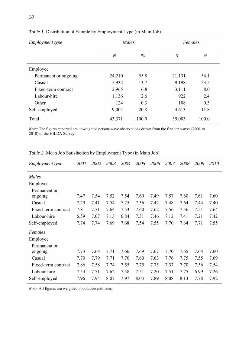
28

Table 1. Distribution of Sample by Employment Type (in Main Job)

Employment type Males Females

N % N %

Employee

Permanent or ongoing 24,210 55.8 21,131 54.1

Casual 5,932 13.7 9,198 23.5

Fixed-term contract 2,965 6.8 3,111 8.0

Labour-hire 1,136 2.6 922 2.4

Other 124 0.3 108 0.3

Self-employed 9,004 20.8 4,613 11.8

Total 43,371 100.0 39,083 100.0

Note: The figures reported are unweighted person-wave observations drawn from the first ten waves (2001 to 2010) of the HILDA Survey.

Table 2. Mean Job Satisfaction by Employment Type (in Main Job)

Employment type 2001 2002 2003 2004 2005 2006 2007 2008 2009 2010

Males

Employee

Permanent or ongoing 7.47 7.54 7.52 7.54 7.60 7.49 7.57 7.60 7.61 7.60

Casual 7.29 7.41 7.54 7.25 7.36 7.42 7.48 7.64 7.44 7.40

Fixed-term contract 7.81 7.71 7.64 7.53 7.60 7.62 7.56 7.56 7.51 7.64

Labour-hire 6.59 7.07 7.13 6.84 7.31 7.46 7.12 7.41 7.21 7.42

Self-employed 7.74 7.74 7.69 7.68 7.54 7.55 7.70 7.64 7.71 7.55

Females

Employee

Permanent or ongoing 7.73 7.64 7.71 7.66 7.69 7.67 7.70 7.65 7.64 7.60

Casual 7.70 7.79 7.71 7.70 7.60 7.63 7.76 7.75 7.55 7.69

Fixed-term contract 7.86 7.58 7.74 7.55 7.75 7.75 7.37 7.70 7.56 7.54

Labour-hire 7.54 7.71 7.62 7.58 7.51 7.20 7.51 7.75 6.99 7.26

Self-employed 7.96 7.94 8.07 7.97 8.03 7.89 8.08 8.13 7.78 7.92

Note: All figures are weighted population estimates.

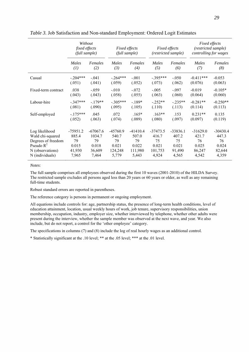
29

Table 3. Job Satisfaction and Non-standard Employment: Ordered Logit Estimates

Without fixed effects (full sample)

Fixed effects (full sample)

Fixed effects

(restricted sample)

Fixed effects (restricted sample)

controlling for wages

Males (1)

Females(2)

Males (3)

Females(4)

Males (5)

Females (6)

Males (7)

Females(8)

Casual -.204*** (.051)

-.041 (.041)

-.264***(.059)

-.001 (.052)

-.395***(.073)

-.050 (.062)

-0.411***(0.076)

-0.053 (0.063)

Fixed-term contract .038 (.043)

-.059 (.043)

-.010 (.058)

-.072 (.055)

-.005 (.063)

-.097 (.060)

-0.019 (0.064)

-0.105* (0.060)

Labour-hire -.347*** (.081)

-.179**(.090)

-.305***(.095)

-.189* (.105)

-.252**(.110)

-.235** (.113)

-0.281** (0.114)

-0.250**(0.113)

Self-employed -.175*** (.052)

.045 (.063)

.072 (.074)

.165* (.089)

.163**(.080)

.153 (.097)

0.231** (0.097)

0.135 (0.119)

Log likelihood -75951.2 -67067.6 -45760.9 -41410.4 -37473.5 -33836.1 -31629.0 -30430.4 Wald chi-squared 885.4 1034.7 540.7 507.0 416.7 407.2 421.7 447.3 Degrees of freedom 79 79 79 79 75 75 76 76 Pseudo R2 0.015 0.018 0.021 0.022 0.021 0.021 0.025 0.024 N (observations) 41,930 36,609 124,248 111,980 101,753 91,490 86,247 82,644 N (individuals) 7,965 7,464 5,779 5,443 4,924 4,565 4,542 4,359

Notes:

The full sample comprises all employees observed during the first 10 waves (2001-2010) of the HILDA Survey. The restricted sample excludes all persons aged less than 20 years or 60 years or older, as well as any remaining full-time students.

Robust standard errors are reported in parentheses.

The reference category is persons in permanent or ongoing employment.

All equations include controls for: age, partnership status, the presence of long-term health conditions, level of education attainment, location, usual weekly hours of work, job tenure, supervisory responsibilities, union membership, occupation, industry, employer size, whether interviewed by telephone, whether other adults were present during the interview, whether the sample member was observed at the next wave, and year. We also include, but do not report, a control for the ‘other employee’ category.

The specifications in columns (7) and (8) include the log of real hourly wages as an additional control.

* Statistically significant at the .10 level; ** at the .05 level; *** at the .01 level.

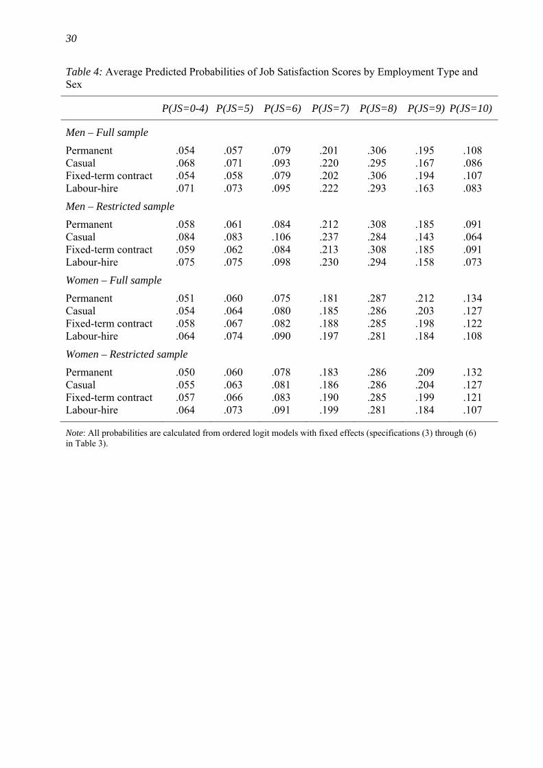
30

Table 4: Average Predicted Probabilities of Job Satisfaction Scores by Employment Type and Sex

P(JS=0-4) P(JS=5) P(JS=6) P(JS=7) P(JS=8) P(JS=9) P(JS=10)

Men – Full sample

Permanent .054 .057 .079 .201 .306 .195 .108 Casual .068 .071 .093 .220 .295 .167 .086 Fixed-term contract .054 .058 .079 .202 .306 .194 .107 Labour-hire .071 .073 .095 .222 .293 .163 .083

Men – Restricted sample

Permanent .058 .061 .084 .212 .308 .185 .091 Casual .084 .083 .106 .237 .284 .143 .064 Fixed-term contract .059 .062 .084 .213 .308 .185 .091 Labour-hire .075 .075 .098 .230 .294 .158 .073

Women – Full sample

Permanent .051 .060 .075 .181 .287 .212 .134 Casual .054 .064 .080 .185 .286 .203 .127 Fixed-term contract .058 .067 .082 .188 .285 .198 .122 Labour-hire .064 .074 .090 .197 .281 .184 .108

Women – Restricted sample

Permanent .050 .060 .078 .183 .286 .209 .132 Casual .055 .063 .081 .186 .286 .204 .127 Fixed-term contract .057 .066 .083 .190 .285 .199 .121 Labour-hire .064 .073 .091 .199 .281 .184 .107

Note: All probabilities are calculated from ordered logit models with fixed effects (specifications (3) through (6) in Table 3).

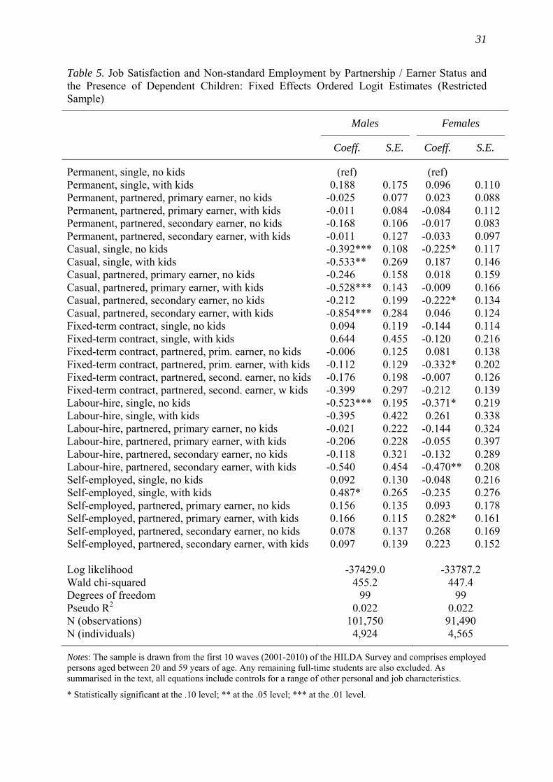
31

Table 5. Job Satisfaction and Non-standard Employment by Partnership / Earner Status and the Presence of Dependent Children: Fixed Effects Ordered Logit Estimates (Restricted Sample)

Males Females

Coeff. S.E. Coeff. S.E.

Permanent, single, no kids (ref) (ref) Permanent, single, with kids 0.188 0.175 0.096 0.110 Permanent, partnered, primary earner, no kids -0.025 0.077 0.023 0.088 Permanent, partnered, primary earner, with kids -0.011 0.084 -0.084 0.112 Permanent, partnered, secondary earner, no kids -0.168 0.106 -0.017 0.083 Permanent, partnered, secondary earner, with kids -0.011 0.127 -0.033 0.097 Casual, single, no kids -0.392*** 0.108 -0.225* 0.117 Casual, single, with kids -0.533** 0.269 0.187 0.146 Casual, partnered, primary earner, no kids -0.246 0.158 0.018 0.159 Casual, partnered, primary earner, with kids -0.528*** 0.143 -0.009 0.166 Casual, partnered, secondary earner, no kids -0.212 0.199 -0.222* 0.134 Casual, partnered, secondary earner, with kids -0.854*** 0.284 0.046 0.124 Fixed-term contract, single, no kids 0.094 0.119 -0.144 0.114 Fixed-term contract, single, with kids 0.644 0.455 -0.120 0.216 Fixed-term contract, partnered, prim. earner, no kids -0.006 0.125 0.081 0.138 Fixed-term contract, partnered, prim. earner, with kids -0.112 0.129 -0.332* 0.202 Fixed-term contract, partnered, second. earner, no kids -0.176 0.198 -0.007 0.126 Fixed-term contract, partnered, second. earner, w kids -0.399 0.297 -0.212 0.139 Labour-hire, single, no kids -0.523*** 0.195 -0.371* 0.219 Labour-hire, single, with kids -0.395 0.422 0.261 0.338 Labour-hire, partnered, primary earner, no kids -0.021 0.222 -0.144 0.324 Labour-hire, partnered, primary earner, with kids -0.206 0.228 -0.055 0.397 Labour-hire, partnered, secondary earner, no kids -0.118 0.321 -0.132 0.289 Labour-hire, partnered, secondary earner, with kids -0.540 0.454 -0.470** 0.208 Self-employed, single, no kids 0.092 0.130 -0.048 0.216 Self-employed, single, with kids 0.487* 0.265 -0.235 0.276 Self-employed, partnered, primary earner, no kids 0.156 0.135 0.093 0.178 Self-employed, partnered, primary earner, with kids 0.166 0.115 0.282* 0.161 Self-employed, partnered, secondary earner, no kids 0.078 0.137 0.268 0.169 Self-employed, partnered, secondary earner, with kids 0.097 0.139 0.223 0.152 Log likelihood -37429.0 -33787.2 Wald chi-squared 455.2 447.4 Degrees of freedom 99 99 Pseudo R2 0.022 0.022 N (observations) 101,750 91,490 N (individuals) 4,924 4,565

Notes: The sample is drawn from the first 10 waves (2001-2010) of the HILDA Survey and comprises employed persons aged between 20 and 59 years of age. Any remaining full-time students are also excluded. As summarised in the text, all equations include controls for a range of other personal and job characteristics.

* Statistically significant at the .10 level; ** at the .05 level; *** at the .01 level.

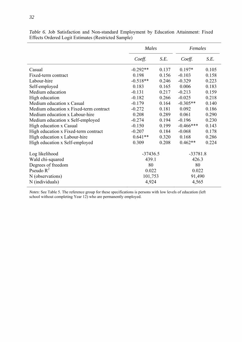
32

Table 6. Job Satisfaction and Non-standard Employment by Education Attainment: Fixed Effects Ordered Logit Estimates (Restricted Sample)

Males Females

Coeff. S.E. Coeff. S.E.

Casual -0.292** 0.137 0.197* 0.105 Fixed-term contract 0.198 0.156 -0.103 0.158 Labour-hire -0.518** 0.246 -0.329 0.223 Self-employed 0.183 0.165 0.006 0.183 Medium education -0.131 0.217 -0.213 0.159 High education -0.182 0.266 -0.025 0.218 Medium education x Casual -0.179 0.164 -0.305** 0.140 Medium education x Fixed-term contract -0.272 0.181 0.092 0.186 Medium education x Labour-hire 0.208 0.289 0.061 0.290 Medium education x Self-employed -0.274 0.194 -0.196 0.230 High education x Casual -0.150 0.199 -0.466*** 0.143 High education x Fixed-term contract -0.207 0.184 -0.068 0.178 High education x Labour-hire 0.641** 0.320 0.168 0.286 High education x Self-employed 0.309 0.208 0.462** 0.224 Log likelihood -37436.5 -33781.8 Wald chi-squared 439.1 426.3 Degrees of freedom 80 80 Pseudo R2 0.022 0.022 N (observations) 101,753 91,490 N (individuals) 4,924 4,565

Notes: See Table 5. The reference group for these specifications is persons with low levels of education (left school without completing Year 12) who are permanently employed.

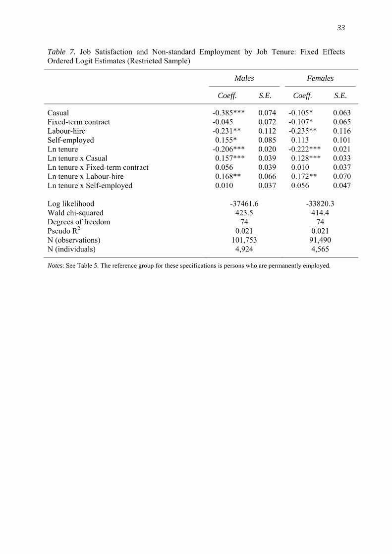
33

Table 7. Job Satisfaction and Non-standard Employment by Job Tenure: Fixed Effects Ordered Logit Estimates (Restricted Sample)

Males Females

Coeff. S.E. Coeff. S.E.

Casual -0.385*** 0.074 -0.105* 0.063 Fixed-term contract -0.045 0.072 -0.107* 0.065 Labour-hire -0.231** 0.112 -0.235** 0.116 Self-employed 0.155* 0.085 0.113 0.101 Ln tenure -0.206*** 0.020 -0.222*** 0.021 Ln tenure x Casual 0.157*** 0.039 0.128*** 0.033 Ln tenure x Fixed-term contract 0.056 0.039 0.010 0.037 Ln tenure x Labour-hire 0.168** 0.066 0.172** 0.070 Ln tenure x Self-employed 0.010 0.037 0.056 0.047 Log likelihood -37461.6 -33820.3 Wald chi-squared 423.5 414.4 Degrees of freedom 74 74 Pseudo R2 0.021 0.021 N (observations) 101,753 91,490 N (individuals) 4,924 4,565

Notes: See Table 5. The reference group for these specifications is persons who are permanently employed.

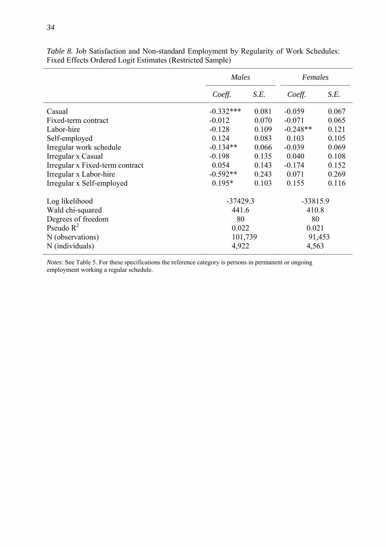
34

Table 8. Job Satisfaction and Non-standard Employment by Regularity of Work Schedules: Fixed Effects Ordered Logit Estimates (Restricted Sample)

Males Females

Coeff. S.E. Coeff. S.E.

Casual -0.332*** 0.081 -0.059 0.067 Fixed-term contract -0.012 0.070 -0.071 0.065 Labor-hire -0.128 0.109 -0.248** 0.121 Self-employed 0.124 0.083 0.103 0.105 Irregular work schedule -0.134** 0.066 -0.039 0.069 Irregular x Casual -0.198 0.135 0.040 0.108 Irregular x Fixed-term contract 0.054 0.143 -0.174 0.152 Irregular x Labor-hire -0.592** 0.243 0.071 0.269 Irregular x Self-employed 0.195* 0.103 0.155 0.116 Log likelihood -37429.3 -33815.9 Wald chi-squared 441.6 410.8 Degrees of freedom 80 80 Pseudo R2 0.022 0.021 N (observations) 101,739 91,453 N (individuals) 4,922 4,563

Notes: See Table 5. For these specifications the reference category is persons in permanent or ongoing employment working a regular schedule.

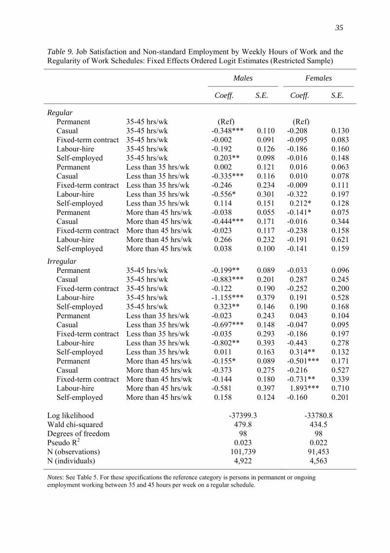
35

Table 9. Job Satisfaction and Non-standard Employment by Weekly Hours of Work and the Regularity of Work Schedules: Fixed Effects Ordered Logit Estimates (Restricted Sample)

Males Females

Coeff. S.E. Coeff. S.E.

Regular Permanent 35-45 hrs/wk (Ref) (Ref) Casual 35-45 hrs/wk -0.348*** 0.110 -0.208 0.130 Fixed-term contract 35-45 hrs/wk -0.002 0.091 -0.095 0.083 Labour-hire 35-45 hrs/wk -0.192 0.126 -0.186 0.160 Self-employed 35-45 hrs/wk 0.203** 0.098 -0.016 0.148 Permanent Less than 35 hrs/wk 0.002 0.121 0.016 0.063 Casual Less than 35 hrs/wk -0.335*** 0.116 0.010 0.078 Fixed-term contract Less than 35 hrs/wk -0.246 0.234 -0.009 0.111 Labour-hire Less than 35 hrs/wk -0.556* 0.301 -0.322 0.197 Self-employed Less than 35 hrs/wk 0.114 0.151 0.212* 0.128 Permanent More than 45 hrs/wk -0.038 0.055 -0.141* 0.075 Casual More than 45 hrs/wk -0.444*** 0.171 -0.016 0.344 Fixed-term contract More than 45 hrs/wk -0.023 0.117 -0.238 0.158 Labour-hire More than 45 hrs/wk 0.266 0.232 -0.191 0.621 Self-employed More than 45 hrs/wk 0.038 0.100 -0.141 0.159

Irregular Permanent 35-45 hrs/wk -0.199** 0.089 -0.033 0.096 Casual 35-45 hrs/wk -0.883*** 0.201 0.287 0.245 Fixed-term contract 35-45 hrs/wk -0.122 0.190 -0.252 0.200 Labour-hire 35-45 hrs/wk -1.155*** 0.379 0.191 0.528 Self-employed 35-45 hrs/wk 0.323** 0.146 0.190 0.168 Permanent Less than 35 hrs/wk -0.023 0.243 0.043 0.104 Casual Less than 35 hrs/wk -0.697*** 0.148 -0.047 0.095 Fixed-term contract Less than 35 hrs/wk -0.035 0.293 -0.186 0.197 Labour-hire Less than 35 hrs/wk -0.802** 0.393 -0.443 0.278 Self-employed Less than 35 hrs/wk 0.011 0.163 0.314** 0.132 Permanent More than 45 hrs/wk -0.155* 0.089 -0.501*** 0.171 Casual More than 45 hrs/wk -0.373 0.275 -0.216 0.527 Fixed-term contract More than 45 hrs/wk -0.144 0.180 -0.731** 0.339 Labour-hire More than 45 hrs/wk -0.581 0.397 1.893*** 0.710 Self-employed More than 45 hrs/wk 0.158 0.124 -0.160 0.201

Log likelihood -37399.3 -33780.8 Wald chi-squared 479.8 434.5 Degrees of freedom 98 98 Pseudo R2 0.023 0.022 N (observations) 101,739 91,453 N (individuals) 4,922 4,563

Notes: See Table 5. For these specifications the reference category is persons in permanent or ongoing employment working between 35 and 45 hours per week on a regular schedule.

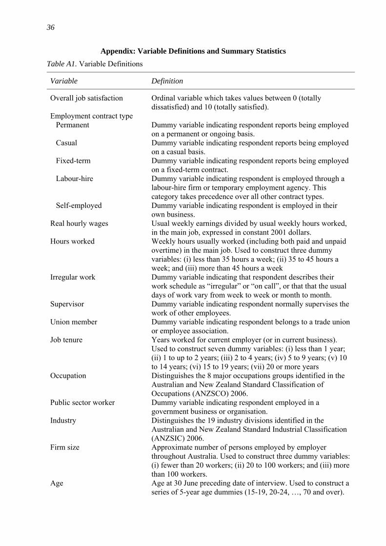
36

Appendix: Variable Definitions and Summary Statistics

Table A1. Variable Definitions

Variable Definition

Overall job satisfaction Ordinal variable which takes values between 0 (totally dissatisfied) and 10 (totally satisfied).

Employment contract type Permanent Dummy variable indicating respondent reports being employed

on a permanent or ongoing basis. Casual Dummy variable indicating respondent reports being employed

on a casual basis. Fixed-term Dummy variable indicating respondent reports being employed

on a fixed-term contract. Labour-hire Dummy variable indicating respondent is employed through a

labour-hire firm or temporary employment agency. This category takes precedence over all other contract types.

Self-employed Dummy variable indicating respondent is employed in their own business.

Real hourly wages Usual weekly earnings divided by usual weekly hours worked, in the main job, expressed in constant 2001 dollars.

Hours worked Weekly hours usually worked (including both paid and unpaid overtime) in the main job. Used to construct three dummy variables: (i) less than 35 hours a week; (ii) 35 to 45 hours a week; and (iii) more than 45 hours a week

Irregular work Dummy variable indicating that respondent describes their work schedule as “irregular” or “on call”, or that that the usual days of work vary from week to week or month to month.

Supervisor Dummy variable indicating respondent normally supervises the work of other employees.

Union member Dummy variable indicating respondent belongs to a trade union or employee association.

Job tenure Years worked for current employer (or in current business). Used to construct seven dummy variables: (i) less than 1 year; (ii) 1 to up to 2 years; (iii) 2 to 4 years; (iv) 5 to 9 years; (v) 10 to 14 years; (vi) 15 to 19 years; (vii) 20 or more years

Occupation Distinguishes the 8 major occupations groups identified in the Australian and New Zealand Standard Classification of Occupations (ANZSCO) 2006.

Public sector worker Dummy variable indicating respondent employed in a government business or organisation.

Industry Distinguishes the 19 industry divisions identified in the Australian and New Zealand Standard Industrial Classification (ANZSIC) 2006.

Firm size Approximate number of persons employed by employer throughout Australia. Used to construct three dummy variables: (i) fewer than 20 workers; (ii) 20 to 100 workers; and (iii) more than 100 workers.

Age Age at 30 June preceding date of interview. Used to construct a series of 5-year age dummies (15-19, 20-24, …, 70 and over).

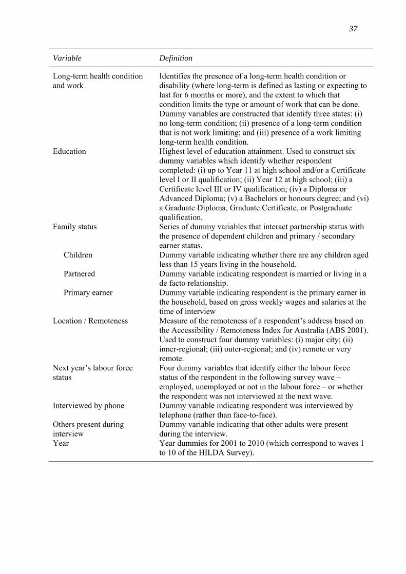
37

Variable Definition

Long-term health condition and work

Identifies the presence of a long-term health condition or disability (where long-term is defined as lasting or expecting to last for 6 months or more), and the extent to which that condition limits the type or amount of work that can be done. Dummy variables are constructed that identify three states: (i) no long-term condition; (ii) presence of a long-term condition that is not work limiting; and (iii) presence of a work limiting long-term health condition.

Education Highest level of education attainment. Used to construct six dummy variables which identify whether respondent completed: (i) up to Year 11 at high school and/or a Certificate level I or II qualification; (ii) Year 12 at high school; (iii) a Certificate level III or IV qualification; (iv) a Diploma or Advanced Diploma; (v) a Bachelors or honours degree; and (vi) a Graduate Diploma, Graduate Certificate, or Postgraduate qualification.

Family status Series of dummy variables that interact partnership status with the presence of dependent children and primary / secondary earner status.

Children Dummy variable indicating whether there are any children aged less than 15 years living in the household.

Partnered Dummy variable indicating respondent is married or living in a de facto relationship.

Primary earner Dummy variable indicating respondent is the primary earner in the household, based on gross weekly wages and salaries at the time of interview

Location / Remoteness Measure of the remoteness of a respondent’s address based on the Accessibility / Remoteness Index for Australia (ABS 2001). Used to construct four dummy variables: (i) major city; (ii) inner-regional; (iii) outer-regional; and (iv) remote or very remote.

Next year’s labour force status

Four dummy variables that identify either the labour force status of the respondent in the following survey wave – employed, unemployed or not in the labour force – or whether the respondent was not interviewed at the next wave.

Interviewed by phone Dummy variable indicating respondent was interviewed by telephone (rather than face-to-face).

Others present during interview

Dummy variable indicating that other adults were present during the interview.

Year Year dummies for 2001 to 2010 (which correspond to waves 1 to 10 of the HILDA Survey).

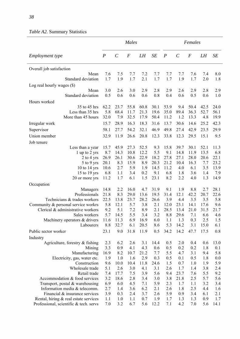
38

Table A2. Summary Statistics

Males Females

Employment type P C F LH SE P C F LH SE

Overall job satisfaction Mean 7.6 7.5 7.7 7.2 7.7 7.7 7.7 7.6 7.4 8.0

Standard deviation 1.7 1.9 1.7 2.1 1.7 1.7 1.9 1.7 2.0 1.8

Log real hourly wages ($) Mean 3.0 2.6 3.0 2.9 2.8 2.9 2.6 2.9 2.8 2.9

Standard deviation 0.5 0.6 0.6 0.6 0.8 0.4 0.6 0.5 0.6 1.0

Hours worked 35 to 45 hrs 62.2 23.7 55.8 60.8 30.1 53.9 9.4 50.4 42.5 24.0

Less than 35 hrs 5.8 68.4 11.7 21.3 19.6 35.0 89.4 36.3 52.7 56.1More than 45 hours 32.0 7.9 32.5 17.9 50.4 11.2 1.2 13.3 4.8 19.9

Irregular work 15.7 28.9 16.3 18.3 31.6 13.7 30.6 14.6 25.2 42.3

Supervisor 58.1 27.7 54.2 32.1 46.9 49.8 27.4 42.9 23.5 29.9

Union member 32.9 11.9 26.6 20.8 12.3 33.8 12.3 29.5 15.1 9.5

Job tenure Less than a year 15.7 45.9 27.3 52.5 9.3 15.8 39.7 30.1 52.1 11.3

1 up to 2 yrs 8.7 14.3 10.8 12.2 5.5 9.1 14.8 11.9 13.5 6.82 to 4 yrs 26.9 26.1 30.6 22.9 18.2 27.8 27.1 28.0 20.6 22.15 to 9 yrs 20.1 8.3 15.9 8.9 20.3 21.2 10.4 16.3 7.7 23.2

10 to 14 yrs 10.6 2.7 5.9 1.9 14.5 11.2 4.0 6.1 3.5 13.915 to 19 yrs 6.8 1.1 3.4 0.2 9.1 6.8 1.8 3.6 1.4 7.9

20 or more yrs 11.2 1.7 6.1 1.5 23.1 8.2 2.2 4.0 1.3 14.9

Occupation Managers 14.8 2.2 16.0 4.7 31.9 9.1 1.9 8.8 2.7 28.1

Professionals 21.8 8.3 29.0 13.6 19.5 31.4 12.1 42.2 20.7 22.6Technicians & trades workers 22.5 13.8 23.7 28.2 26.6 3.9 4.4 3.5 3.5 5.8

Community & personal service workrs 5.8 12.1 5.7 3.8 2.1 12.0 23.1 14.1 17.6 9.6Clerical & administrative workers 9.2 5.1 7.2 8.9 2.1 28.5 13.4 21.0 31.5 21.7

Sales workers 5.7 14.5 5.5 3.4 3.2 8.8 29.6 7.1 6.6 4.6Machinery operators & drivers 11.6 11.3 6.9 16.9 6.0 1.1 1.3 0.3 2.5 1.5

Labourers 8.8 32.7 6.1 20.5 8.6 5.3 14.2 3.1 15.0 6.1

Public sector worker 23.1 9.0 31.8 11.9 0.5 34.2 14.2 47.7 17.5 0.8

Industry Agriculture, forestry & fishing 2.3 6.2 2.6 3.1 14.4 0.5 2.0 0.4 0.6 13.0

Mining 3.3 0.9 4.1 4.3 0.6 0.5 0.2 0.2 1.8 0.1Manufacturing 16.9 8.2 10.7 21.2 7.7 5.5 4.7 3.1 9.4 5.8

Electricity, gas, water etc. 1.9 1.0 1.6 2.9 0.3 0.5 0.1 0.5 1.8 0.0Construction 9.6 10.0 10.4 11.8 24.6 1.5 0.7 1.0 1.9 5.9

Wholesale trade 5.1 2.6 3.0 4.1 3.1 2.6 1.7 1.4 3.8 2.4Retail trade 7.4 17.7 7.5 3.9 5.6 9.4 23.7 7.6 5.5 9.2

Accommodation & food services 3.2 18.6 2.8 3.4 3.0 3.8 21.8 2.5 5.7 5.6Transport, postal & warehousing 6.9 6.0 4.5 7.1 5.9 2.3 1.7 1.1 3.2 3.4Information media & telecomm. 2.7 1.4 3.6 6.2 2.1 2.6 1.8 2.5 4.4 1.6

Financial & insurance services 3.9 0.3 2.4 3.7 2.6 5.9 0.9 3.4 6.1 2.1Rental, hiring & real estate services 1.1 1.0 1.1 0.7 1.9 1.7 1.3 1.3 0.9 1.7

Professional, scientific & tech. servs 7.0 3.2 6.7 5.6 12.2 7.1 4.2 7.0 5.6 14.1

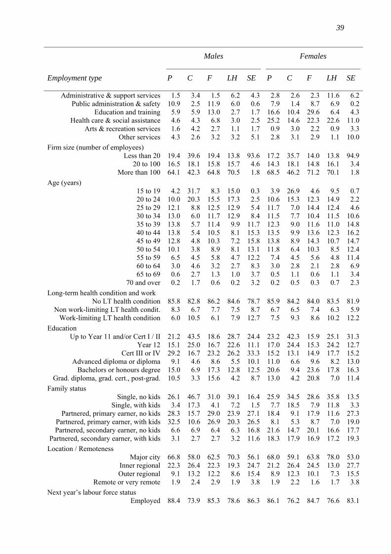
39

Males Females

Employment type P C F LH SE P C F LH SE

Administrative & support services 1.5 3.4 1.5 6.2 4.3 2.8 2.6 2.3 11.6 6.2Public administration & safety 10.9 2.5 11.9 6.0 0.6 7.9 1.4 8.7 6.9 0.2

Education and training 5.9 5.9 13.0 2.7 1.7 16.6 10.4 29.6 6.4 4.3Health care & social assistance 4.6 4.3 6.8 3.0 2.5 25.2 14.6 22.3 22.6 11.0

Arts & recreation services 1.6 4.2 2.7 1.1 1.7 0.9 3.0 2.2 0.9 3.3Other services 4.3 2.6 3.2 3.2 5.1 2.8 3.1 2.9 1.1 10.0

Firm size (number of employees) Less than 20 19.4 39.6 19.4 13.8 93.6 17.2 35.7 14.0 13.8 94.9

20 to 100 16.5 18.1 15.8 15.7 4.6 14.3 18.1 14.8 16.1 3.4More than 100 64.1 42.3 64.8 70.5 1.8 68.5 46.2 71.2 70.1 1.8

Age (years) 15 to 19 4.2 31.7 8.3 15.0 0.3 3.9 26.9 4.6 9.5 0.720 to 24 10.0 20.3 15.5 17.3 2.5 10.6 15.3 12.3 14.9 2.225 to 29 12.1 8.8 12.5 12.9 5.4 11.7 7.0 14.4 12.4 4.630 to 34 13.0 6.0 11.7 12.9 8.4 11.5 7.7 10.4 11.5 10.635 to 39 13.8 5.7 11.4 9.9 11.7 12.3 9.0 11.6 11.0 14.840 to 44 13.8 5.4 10.5 8.1 15.3 13.5 9.9 13.6 12.3 16.245 to 49 12.8 4.8 10.3 7.2 15.8 13.8 8.9 14.3 10.7 14.750 to 54 10.1 3.8 8.9 8.1 13.1 11.8 6.4 10.3 8.5 12.455 to 59 6.5 4.5 5.8 4.7 12.2 7.4 4.5 5.6 4.8 11.460 to 64 3.0 4.6 3.2 2.7 8.3 3.0 2.8 2.1 2.8 6.965 to 69 0.6 2.7 1.3 1.0 3.7 0.5 1.1 0.6 1.1 3.4

70 and over 0.2 1.7 0.6 0.2 3.2 0.2 0.5 0.3 0.7 2.3

Long-term health condition and work No LT health condition 85.8 82.8 86.2 84.6 78.7 85.9 84.2 84.0 83.5 81.9

Non work-limiting LT health condit. 8.3 6.7 7.7 7.5 8.7 6.7 6.5 7.4 6.3 5.9Work-limiting LT health condition 6.0 10.5 6.1 7.9 12.7 7.5 9.3 8.6 10.2 12.2

Education Up to Year 11 and/or Cert I / II 21.2 43.5 18.6 28.7 24.4 23.2 42.3 15.9 25.1 31.3

Year 12 15.1 25.0 16.7 22.6 11.1 17.0 24.4 15.3 24.2 12.7Cert III or IV 29.2 16.7 23.2 26.2 33.3 15.2 13.1 14.9 17.7 15.2

Advanced diploma or diploma 9.1 4.6 8.6 5.5 10.1 11.0 6.6 9.6 8.2 13.0Bachelors or honours degree 15.0 6.9 17.3 12.8 12.5 20.6 9.4 23.6 17.8 16.3

Grad. diploma, grad. cert., post-grad. 10.5 3.3 15.6 4.2 8.7 13.0 4.2 20.8 7.0 11.4

Family status Single, no kids 26.1 46.7 31.0 39.1 16.4 25.9 34.5 28.6 35.8 13.5

Single, with kids 3.4 17.3 4.1 7.2 1.5 7.7 18.5 7.9 11.8 3.3Partnered, primary earner, no kids 28.3 15.7 29.0 23.9 27.1 18.4 9.1 17.9 11.6 27.3

Partnered, primary earner, with kids 32.5 10.6 26.9 20.3 26.5 8.1 5.3 8.7 7.0 19.0Partnered, secondary earner, no kids 6.6 6.9 6.4 6.3 16.8 21.6 14.7 20.1 16.6 17.7

Partnered, secondary earner, with kids 3.1 2.7 2.7 3.2 11.6 18.3 17.9 16.9 17.2 19.3

Location / Remoteness Major city 66.8 58.0 62.5 70.3 56.1 68.0 59.1 63.8 78.0 53.0

Inner regional 22.3 26.4 22.3 19.3 24.7 21.2 26.4 24.5 13.0 27.7Outer regional 9.1 13.2 12.2 8.6 15.4 8.9 12.3 10.1 7.3 15.5

Remote or very remote 1.9 2.4 2.9 1.9 3.8 1.9 2.2 1.6 1.7 3.8

Next year’s labour force status Employed 88.4 73.9 85.3 78.6 86.3 86.1 76.2 84.7 76.6 83.1

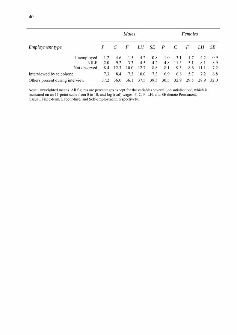
40

Males Females

Employment type P C F LH SE P C F LH SE

Unemployed 1.2 4.6 1.5 4.2 0.8 1.0 3.1 1.7 4.2 0.9NILF 2.0 9.2 3.3 4.5 4.2 4.8 11.3 5.1 8.1 8.9

Not observed 8.4 12.3 10.0 12.7 8.8 8.1 9.5 8.6 11.1 7.2

Interviewed by telephone 7.3 8.4 7.3 10.0 7.3 6.9 6.8 5.7 7.2 6.8

Others present during interview 37.2 36.0 36.1 37.5 39.3 30.5 32.9 29.5 28.9 32.0

Note: Unweighted means. All figures are percentages except for the variables ‘overall job satisfaction’, which is measured on an 11-point scale from 0 to 10, and log (real) wages. P, C, F, LH, and SE denote Permanent, Casual, Fixed-term, Labour-hire, and Self-employment, respectively.