Moritz A. Drupp

Limits to substitution between ecosystem services and manufactured goods and implications for social discounting Article (Accepted version) (Refereed)

Original citation: Drupp, Moritz A. (2016) Limits to substitution between ecosystem services and manufactured goods and implications for social discounting. Environmental and Resource Economics. ISSN 0924-6460 DOI: 10.1007/s10640-016-0068-5 © 2016 Springer Science+Business Media Dordrecht This version available at: http://eprints.lse.ac.uk/68298/ Available in LSE Research Online: November 2016 LSE has developed LSE Research Online so that users may access research output of the School. Copyright © and Moral Rights for the papers on this site are retained by the individual authors and/or other copyright owners. Users may download and/or print one copy of any article(s) in LSE Research Online to facilitate their private study or for non-commercial research. You may not engage in further distribution of the material or use it for any profit-making activities or any commercial gain. You may freely distribute the URL (http://eprints.lse.ac.uk) of the LSE Research Online website. This document is the author’s final accepted version of the journal article. There may be differences between this version and the published version. You are advised to consult the publisher’s version if you wish to cite from it.

forthcoming in: Environmental and Resource Economics

Limits to Substitution

between Ecosystem Services and Manufactured

Goods and Implications for Social Discounting

Moritz A. Druppa ,b ,∗ , ‡

a Department of Economics, University of Kiel, Germanyb Department of Geography and Environment,

London School of Economics and Political Science, UK

Abstract: This paper examines implications of limits to substitution for estimating

substitutability between ecosystem services and manufactured goods and for social dis-

counting. Based on a model that accounts for a subsistence requirement in the consump-

tion of ecosystem services, we provide empirical evidence on substitution elasticities. We

�nd an initial mean elasticity of substitution of two, which declines over time towards

complementarity. We subsequently extend the theory of dual discounting by introduc-

ing a subsistence requirement. The relative price of ecosystem services is non-constant

and grows without bound as the consumption of ecosystem services declines towards the

subsistence level. An application suggests that the initial discount rate for ecosystem

services is more than a percentage-point lower as compared to manufactured goods. This

di�erence increases by a further half percentage-point over a 300-year time horizon. The

results underscore the importance of considering limited substitutability in long-term

public project appraisal.

JEL-Classi�cation: Q01, Q57, H43, D61, D90

Keywords: Limited substitutability; Dual discounting; Ecosystem services; Subsis-

tence; Project evaluation; Sustainability

∗Correspondence: Department of Economics, University of Kiel, Wilhelm-Seelig-Platz 1, 24118 Kiel,

Germany. Email: Drupp@economics.uni-kiel.de; Phone: +49-431-880-4986.

‡I am very grateful to Stefan Baumgärtner, Ben Groom and Martin Quaas for their support. Fur-

thermore I thank Mikolaj Czajkowski, Simon Dietz, Reyer Gerlagh, Christian Gollier, David Löw-Beer,

Frikk Nesje, Eric Neumayer, Martin Persson, Paolo Piacquadio, Till Requate, Felix Schläpfer, Gregor

Schwerho�, Thomas Sterner and participants at the 2014 SURED, the 2014 WCERE and the IfW

Centenary Conference for helpful comments. Financial support from the German National Academic

Foundation, the DAAD and the BMBF under grant 01LA1104C is gratefully acknowledged.

1

1 Introduction

This paper studies limits to substitution between ecosystem services and manufactured

consumption goods. In particular, we examine implications of a subsistence requirement

in the consumption of ecosystem services for the empirical estimation of the elasticity

of substitution and for the theory and practice of social discounting.

Limited substitutability is a core issue in the debate on sustainable development and

of central importance for environmental and resource management (Gerlagh and van

der Zwaan 2002; Neumayer 2010). The issue of substitutability has recently received

prominent attention in the discussion of dual discounting between ecosystem services

and consumption goods and the economic appraisal of climate change. The debate fol-

lowing the Stern Review (2007) has triggered a rethinking of an adequate speci�cation

of the damages function from climate change (Weitzman 2010), relating in particular to

the adverse impact of climate change on ecosystems and their repercussions for human

well-being (Heal 2009a,b; Neumayer 2007). Sterner and Persson (2008) have shown that

the evaluation of climate damages to utility crucially depends on assumptions regard-

ing substitutability. If future comprehensive consumption is � as is the case in most

integrated assessment models � not valued in relative prices that account for changing

relative scarcities between ecosystem services and manufactured goods, a uniform social

discount rate is inappropriate and dual discounting should be adopted (e.g. Baumgärt-

ner et al. 2015a; Gollier 2010; Guesnerie 2004; Hoel and Sterner 2007; Traeger 2011;

Weikard and Zhu 2005). This is the case when the two goods are less than perfect

substitutes and have diverging growth rates. Baumgärtner et al. (2015a) estimate that

the di�erence in good-speci�c discount rates, also termed `relative price e�ect' (Hoel

and Sterner 2007), amounts to almost a full percentage point.

A survey of experts on social discounting by Drupp et al. (2015) revealed that con-

sidering limited substitutability between ecosystem services and manufactured goods is

one of the most mentioned issues lacking in current discounting guidance. Among the

experts' suggestions on how to improve existing criteria for intergenerational decision-

making are approaches that �set limits in physical terms to the future development that

2

must not be exceeded for reasons of intra- and intergenerational justice [and] use a dis-

counted utilitarian approach to optimize development only within these limits� (Drupp

et al. 2015: 24). A recent proposal on considering such an absolute limit within the

literature on substitutability has been to consider a subsistence requirement or survival

threshold in the consumption of ecosystem services (Heal 2009a,b; Baumgärtner et al.

2015b). At the most basic level one may think of such a subsistence requirement in

terms of minimum consumption levels of water, food and life-enabling ecosystem con-

ditions. Speci�cally, Baumgärtner et al. (2015b) extend the usual constant-elasticity-

of-substitution (CES) framework and show that the elasticity of substitution is non-

constant if there is a subsistence requirement in the consumption of ecosystem services.

A key obstacle to advancing the discussion on limited substitutability � in consump-

tion as well as production � has been the scarcity of empirical evidence (Ayres 2007;

Neumayer 2010; Stern 1997). Recently, Yu and Abler (2010) and Baumgärtner et al.

(2015a) have drawn on a direct relationship within the CES utility speci�cation between

the income elasticity of willingness to pay (WTP) for ecosystem services, a fundamental

substitutability parameter and the elasticity of substitution between ecosystem services

and manufactured goods. They provide estimates for the elasticity of substitution of 5

and 2.63 respectively, suggesting a high degree of substitutability.

This paper makes a twofold contribution to the literature: First, it provides the

most comprehensive account of empirical evidence on substitution elasticities between

ecosystem services and manufactured goods to date and analyses what limits to substitu-

tion imply for the estimation of substitutability. Second, it scrutinises implications of an

absolute limit to substitution in form of a subsistence requirement for social discounting.

For our analysis of empirical evidence on substitutability between ecosystem services

and manufactured goods we employ and extend the model framework of Baumgärtner

et al. (2015b). The subsistence requirement in the consumption of ecosystem services

allows for considering absolute limits to substitution. Furthermore, we draw on the direct

relationship within the CES case between the income elasticity of WTP for ecosystem

services, the substitutability parameter and the elasticity of substitution. While the

elasticity of substitution is non-constant when considering a subsistence requirement,

3

the direct relationship between the income elasticity of WTP and the substitutability

parameter remains. We provide empirical evidence on substitution possibilities based

on income elasticities of WTP from 18 valuation studies. The resulting substitutability

parameters range from -0.16 to 0.86. In the CES case, which holds in cases where there

is an abundant provisioning of ecosystem services or ecosystem services are not required

to meet subsistence needs, this would imply elasticities of substitution of 0.86 to 7.14.

Simple aggregation over all studies yields a mean substitutability parameter of 0.57. We

assume that 15 percent of the initial consumption of ecosystem services is required to

satisfy subsistence needs and use an empirically-founded scenario based on Hoel and

Sterner (2007) and Baumgärtner et al. (2015a) to estimate the time development of the

elasticity of substitution for the empirical sample mean. We �nd an initial value for the

elasticity of substitution of 2, which decreases to 1.56 (0.66) over 150 (300) years.

Subsequently, we explore implications for social discounting of considering absolute

limits to substitution in the form of a subsistence requirement. We extend the standard

dual discounting model (Hoel and Sterner 2007; Traeger 2011) through introducing a

subsistence requirement in the consumption of ecosystem services and analyse the dif-

ference between the good-speci�c discount rates (relative price e�ect). We show that the

relative price e�ect crucially depends on the consumption of ecosystem services relative

to the subsistence requirement. It converges to the CES case, which is determined by

the substitutability parameter and the di�erence in growth rates, if the consumption

of ecosystem services grows over time and becomes plentiful. If, in contrast, the con-

sumption of ecosystem services is limited, the relative price e�ect is non-constant and

depends on the consumption of ecosystem services relative to the subsistence require-

ment. Speci�cally, if ecosystem services are in a continuous decline towards the amount

required for subsistence, the relative price e�ect increases without bound.

We estimate the relative price e�ect for all empirical estimates of the substitutability

parameter using the same scenario analysis and �nd that the initial discount rate for

ecosystem services is on average 1.1 percentage-points lower compared to the rate for

manufactured goods. This di�erence increases by more than half a percentage-point on

average in the longer run due to the subsistence requirement. The case for including

4

ecological discount rates in project evaluation is therefore stronger on average than

previously suggested (Baumgärtner et al. 2015a). A sensitivity analysis further reveals

that the longer-term relative price e�ect is very sensitive to assumptions on the level of

ecosystem services required for subsistence.

Overall, we �nd that it is crucial to consider limits to substitution for the estimation

of the elasticity of substitution between ecosystem services and manufactured goods as

well as for social discounting. A subsistence requirement in the consumption of ecosys-

tem services lowers substitution possibilities and, if ecosystem services are declining,

leads to an increasing relative price of ecosystem services over time. This has important

implications for project evaluation and calls for safeguarding critical ecosystem services.

2 Substitutability of ecosystem services

2.1 Ecosystem services and human well-being

Human well-being fundamentally depends on the vitality of ecosystems and the ecosys-

tem services (ES) they provide (Millennium Ecosystem Assessment (MEA) 2005). While

ecosystem services are necessary constituents of human well-being (Dasgupta 2001),

there is substantial uncertainty and disagreement regarding their importance compared

to manufactured goods and how their provisioning will evolve over time. The MEA

(2005) suggests that 15 of 24 ecosystem service categories have deteriorated, while only

four have improved. Baumgärtner et al. (2015a) estimate, under the assumption that

the single ecosystem service components are part of a homogenous good and using un-

weighted arithmetic means, that global ecosystem services had an average annual loss

rate of 0.52 percent for the period 1950 to 2010. There are a few indicative clues for

the relative contribution of ecosystem services to human well-being. A lower bound

estimate might be the value of food production, which was about 3 percent of global

GDP in 2000 (MEA 2005: 6). The economics of ecosystems and biodiversity (TEEB)

initiative (ten Brink 2011) has calculated that ecosystem service related to agriculture,

forestry and �sheries contribute between 15-20 percent to an adjusted GDP in Brazil,

5

India and Indonesia. This is close to evidence cited in Dasgupta (2010: 7), where the

depreciation of forest, soil and �shery resources in Costa Rica amounted to about 10

percent of GDP. Overall this suggests that the current value-share of ecosystem services

in overall global consumption might be in the range of 3-20 percent.

2.2 Conceptualising and modeling limits to substitution

The question of how limited substitution possibilities between ecosystem services/natural

capital and manufactured goods/capital are is of fundamental importance within envi-

ronmental and resource economics, particularly for the debate on strong versus weak

sustainability (Gerlagh and van der Zwaan 2002; Neumayer 2010). This discussion has

been predominantly set within a CES framework and thus focussed on the value of a

single parameter. Yet, the notion of the elasticity of substitution is much more general

and it is well-known that it need not be constant (Revankar 1971). Conceptual discus-

sions of limits to substitution have concluded that, while there may currently still exist

ample substitution possibilities at the margin, �limits to substitutability in the medium

term at least are real and important� (Ayres 2007: 115); They further argue that these

limits will be strictly binding in the long-run due to thermodynamic limits in the pro-

duction process or subsistence requirements (Ayres 2007; Ehrlich 1989; Heal 2009a,b;

Stern 1997).1 Similarly, Fenichel and Zhao (2014) note that �[in] the limit, society will

not be able to substitute away from clean water, clean air and a number of other natural

resources�. Even if speci�c services were substitutable with technologies, human beings

may still object to substitute them. We thus follow Traeger (2011) in assuming that

limited willingness to substitute in consumption is the ultimately relevant constraint.

To allow for an absolute limit to substitution, we consider a subsistence requirement

in the consumption of ecosystem services. In the related literature, Pezzey and Anderies

(2003) conceptualise subsistence in terms of minimum nutrition levels, whereas Heal

1That is: even though many parts of natural capital and ecosystem services may be replaceable by

technology, Fitter (2013) argues that a number of supporting services (soil formation, water cycling

etc.), selected �nal services (e.g. climate regulation) and goods (e.g. water supply, a safe and enjoyable

environment) may be very hard if not impossible to fully substitute (cf. Ayres 2007).

6

(2009a: 279) notes that �[t]here is a minimum level of ecosystem services needed for

survival�think of this as water, air, and basic foodstu�s�. Other discussants refer to

�essential lifeservices� provided by ecosystems (Traeger 2011: 217) or remark that �a

large part of what the natural environment o�ers us is a necessity� (Dasgupta 2001:

125). While there is no generally accepted notion of subsistence (Steger 2000), Sharif

(1986: 555) argues that it must go beyond a mere consideration of basic physical needs

to encompass the �needs [concerning] physical and mental survival�. Along these lines,

such a subsistence requirement would not only include food, water, bodily security and

more broadly life-enabling ecosystem conditions, but also cultural ecosystem services

like the experience of `naturalness' or the existence of sacred natural environments.

Relatedly, Baumgärtner et al. (2015b: 2) de�ne a subsistence requirement more generally

to �encompass a homogeneous composite good to which an individual attaches absolute

priority before considering trade-o�s with other goods�. Here, we predominantly focus

on a narrower de�nition of subsistence that includes essential services related to the

consumption of water, food, air as well as life-enabling ecosystem conditions.

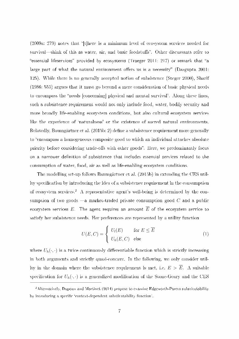
The modelling set-up follows Baumgärtner et al. (2015b) in extending the CES util-

ity speci�cation by introducing the idea of a subsistence requirement in the consumption

of ecosystem services.2 A representative agent's well-being is determined by the con-

sumption of two goods � a market-traded private consumption good C and a public

ecosystem services E. The agent requires an amount E of the ecosystem service to

satisfy her subsistence needs. Her preferences are represented by a utility function

U(E,C) =

Ul(E) for E ≤ E

Uh(E,C) else(1)

where Uh(·, ·) is a twice continuously di�erentiable function which is strictly increasing

in both arguments and strictly quasi-concave. In the following, we only consider util-

ity in the domain where the subsistence requirement is met, i.e. E > E. A suitable

speci�cation for Uh(·, ·) is a generalized modi�cation of the Stone-Geary and the CES

2Alternatively, Dupoux and Martinet (2014) propose to examine Edgeworth-Pareto substitutability

by introducing a speci�c `context-dependent substitutability function'.

7

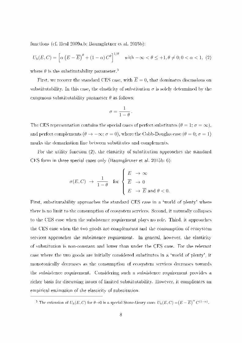
functions (cf. Heal 2009a,b; Baumgärtner et al. 2015b):

Uh(E,C) =[α(E − E

)θ+ (1− α)Cθ

]1/θwith −∞ < θ ≤ +1, θ 6= 0; 0 < α < 1, (2)

where θ is the substitutability parameter.3

First, we recover the standard CES case, with E = 0, that dominates discussions on

substitutability. In this case, the elasticity of substitution σ is solely determined by the

exogenous substitutability parameter θ as follows:

σ =1

1− θ.

The CES representation contains the special cases of perfect substitutes (θ = 1; σ =∞),

and perfect complements (θ → −∞; σ = 0), where the Cobb-Douglas case (θ = 0; σ = 1)

marks the demarkation line between substitutes and complements.

For the utility function (2), the elasticity of substitution approaches the standard

CES form in three special cases only (Baumgärtner et al. 2015b: 6):

σ(E,C) → 1

1− θfor

E → ∞

E → 0

E → E and θ < 0.

First, substitutability approaches the standard CES case in a `world of plenty' where

there is no limit to the consumption of ecosystem services. Second, it naturally collapses

to the CES case when the subsistence requirement plays no role. Third, it approaches

the CES case when the two goods are complements and the consumption of ecosystem

services approaches the subsistence requirement. In general, however, the elasticity

of substitution is non-constant and lower than under the CES case. For the relevant

case where the two goods are initially considered substitutes in a `world of plenty', it

monotonically decreases as the consumption of ecosystem services decreases towards

the subsistence requirement. Considering such a subsistence requirement provides a

richer basis for discussing issues of limited substitutability. However, it complicates an

empirical estimation of the elasticity of substitution.

3 The extension of Uh(E,C) for θ→0 is a special Stone-Geory case: Uh(E,C) =(E − E

)αC(1−α).

8

2.3 Estimating the substitutability of ecosystem services

The substitutability between ecosystem services and manufactured goods, respectively

income, can in principle be elicited using various non-market valuation techniques, such

as choice experiments, contingent valuation or revealed preference approaches.4

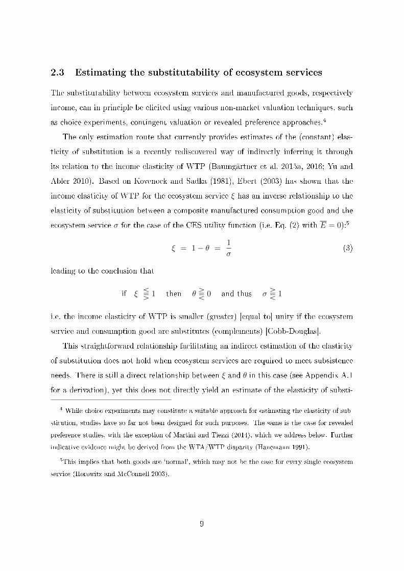
The only estimation route that currently provides estimates of the (constant) elas-

ticity of substitution is a recently rediscovered way of indirectly inferring it through

its relation to the income elasticity of WTP (Baumgärtner et al. 2015a, 2016; Yu and

Abler 2010). Based on Kovenock and Sadka (1981), Ebert (2003) has shown that the

income elasticity of WTP for the ecosystem service ξ has an inverse relationship to the

elasticity of substitution between a composite manufactured consumption good and the

ecosystem service σ for the case of the CES utility function (i.e. Eq. (2) with E = 0):5

ξ = 1− θ =1

σ(3)

leading to the conclusion that

if ξ S 1 then θ T 0 and thus σ T 1

i.e. the income elasticity of WTP is smaller (greater) [equal to] unity if the ecosystem

service and consumption good are substitutes (complements) [Cobb-Douglas].

This straightforward relationship facilitating an indirect estimation of the elasticity

of substitution does not hold when ecosystem services are required to meet subsistence

needs. There is still a direct relationship between ξ and θ in this case (see Appendix A.1

for a derivation), yet this does not directly yield an estimate of the elasticity of substi-

4 While choice experiments may constitute a suitable approach for estimating the elasticity of sub-

stitution, studies have so far not been designed for such purposes. The same is the case for revealed

preference studies, with the exception of Martini and Tiezzi (2014), which we address below. Further

indicative evidence might be derived from the WTA/WTP disparity (Hanemann 1991).

5This implies that both goods are `normal', which may not be the case for every single ecosystem

service (Horowitz and McConnell 2003).

9

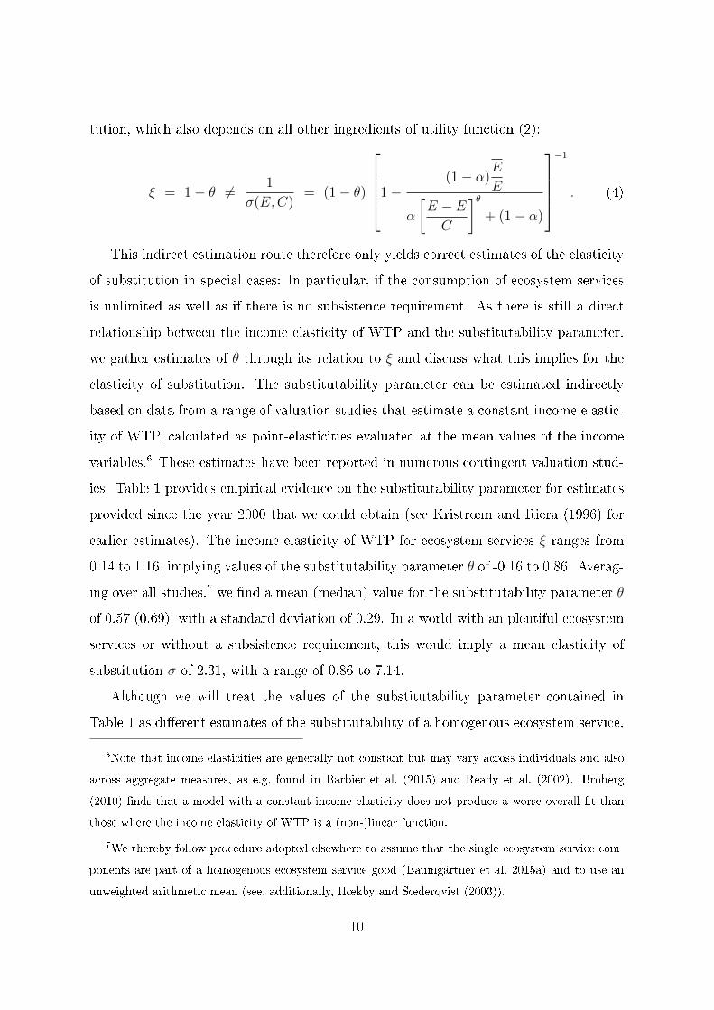
tution, which also depends on all other ingredients of utility function (2):

ξ = 1− θ 6= 1

σ(E,C)= (1− θ)

1−(1− α)

E

E

α

[E − EC

]θ+ (1− α)

−1

. (4)

This indirect estimation route therefore only yields correct estimates of the elasticity

of substitution in special cases: In particular, if the consumption of ecosystem services

is unlimited as well as if there is no subsistence requirement. As there is still a direct

relationship between the income elasticity of WTP and the substitutability parameter,

we gather estimates of θ through its relation to ξ and discuss what this implies for the

elasticity of substitution. The substitutability parameter can be estimated indirectly

based on data from a range of valuation studies that estimate a constant income elastic-

ity of WTP, calculated as point-elasticities evaluated at the mean values of the income

variables.6 These estimates have been reported in numerous contingent valuation stud-

ies. Table 1 provides empirical evidence on the substitutability parameter for estimates

provided since the year 2000 that we could obtain (see Kristr÷m and Riera (1996) for

earlier estimates). The income elasticity of WTP for ecosystem services ξ ranges from

0.14 to 1.16, implying values of the substitutability parameter θ of -0.16 to 0.86. Averag-

ing over all studies,7 we �nd a mean (median) value for the substitutability parameter θ

of 0.57 (0.69), with a standard deviation of 0.29. In a world with an plentiful ecosystem

services or without a subsistence requirement, this would imply a mean elasticity of

substitution σ of 2.31, with a range of 0.86 to 7.14.

Although we will treat the values of the substitutability parameter contained in

Table 1 as di�erent estimates of the substitutability of a homogenous ecosystem service,

6Note that income elasticities are generally not constant but may vary across individuals and also

across aggregate measures, as e.g. found in Barbier et al. (2015) and Ready et al. (2002). Broberg

(2010) �nds that a model with a constant income elasticity does not produce a worse overall �t than

those where the income elasticity of WTP is a (non-)linear function.

7We thereby follow procedure adopted elsewhere to assume that the single ecosystem service com-

ponents are part of a homogenous ecosystem service good (Baumgärtner et al. 2015a) and to use an

unweighted arithmetic mean (see, additionally, H÷kby and S÷derqvist (2003)).

10

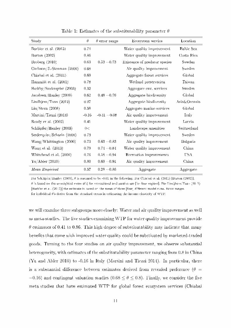
Table 1: Estimates of the substitutability parameter θ

Study θ θ error range Ecosystem service Location

Barbier et al. (2015) 0.74 Water quality improvement Baltic Sea

Barton (2002) 0.86 Water quality improvement Costa Rica

Broberg (2010) 0.63 0.53 � 0.73 Existence of predator species Sweden

Carlsson/J.-Stenman (2000) 0.68 Air quality improvement Sweden

Chiabai et al. (2011) 0.69 Aggregate forest services Global

Hammitt et al. (2001) 0.78 Wetland preservation Taiwan

H÷kby/S÷derqvist (2003) 0.32 Aggregate env. services Sweden

Jacobsen/Hanley (2009) 0.62 0.48 � 0.76 Aggregate biodiversity Global

Lindhjem/Tuan (2012) 0.27 Aggregate biodiversity Asia&Oceania

Liu/Stern (2008) 0.58 Aggregate marine services Global

Martini/Tiezzi (2014) -0.16 -0.41 � 0.08 Air quality improvement Italy

Ready et al. (2002) 0.41 Water quality improvement Latvia

Schläpfer/Hanley (2003) 0< Landscape amenities Switzerland

S÷derqvist/Scharin (2000) 0.73 Water quality improvement Sweden

Wang/Whittington (2000) 0.73 0.63 � 0.83 Air quality improvement Bulgaria

Wang et al. (2013) 0.79 0.74 � 0.84 Water quality improvement China

Whitehead et al. (2000) 0.76 0.58 � 0.94 Recreation improvements USA

Yu/Abler (2010) 0.80 0.69 � 0.91 Air quality improvement China

Mean Empirical 0.57 0.28 � 0.86 Aggregate Aggregate

For Schläpfer/Hanley (2003), θ is assumed to be -0.01 in the following. For Chiabai et al. (2011) [Barton (2002)],

θ is based on the unweighted mean of ξ for recreational and passive use [for four regions]. For Lindjhem/Tuan (2012)

[Barbier et al. (2015)] the estimate is based on the mean of three [four] di�erent model runs. Error ranges

for individual θ's derive from the standard errors in estimating the income elasticity of WTP.

we will examine three subgroups more closely: Water and air quality improvement as well

as meta-studies. The �ve studies examining WTP for water quality improvement provide

θ estimates of 0.41 to 0.86. This high degree of substitutability may indicate that many

bene�ts that come with improved water quality could be substituted by marketed-traded

goods. Turning to the four studies on air quality improvement, we observe substantial

heterogeneity, with estimates of the substitutability parameter ranging from 0.8 in China

(Yu and Abler 2010) to -0.16 in Italy (Martini and Tiezzi 2014). In particular, there

is a substantial di�erence between estimates derived from revealed preference (θ =

−0.16) and contingent valuation studies (0.68 ≤ θ ≤ 0.8). Finally, we consider the �ve

meta-studies that have estimated WTP for global forest ecosystem services (Chiabai

11

et al. 2011), global biodiversity conservation (Jacobsen and Hanley 2009), biodiversity

conservation in Asia and Oceania (Lindhjem and Tuan 2012), global marine ecosystem

services (Liu and Stern 2008) as well as an aggregate environmental service in Sweden

(H÷kby and S÷derqvist 2003). These studies estimate income elasticities ξ in the range

of 0.31 to 0.73, implying values of the substitutability parameter θ of 0.27 to 0.69. The

estimate that comes closest to approximating substitutability of a composite ecosystem

service at the global scale is the meta-study by Jacobsen and Hanley (2009), who gather

145 di�erent WTP estimates from 46 contingent valuation studies across six continents

(Baumgärtner et al. 2015a). They �nd, averaging over the very di�erent biodiversity-

related ecosystem services (i.e. assuming that they are part of a homogeneous good), that

the income elasticity of the WTP for ecosystem services is 0.38 [0.24 to 0.52], implying

a substitutability parameter of 0.62 [0.48 to 0.76]. With an abundant provisioning

of ecosystem services or without a subsistence requirement, this would imply a mean

elasticitiy of substitution of 2.63 [1.92 to 4.17].

We now turn to estimating the elasticity of substitution in a world where ecosystem

services are limited. We simulate the time development of the elasticity of substitution

for an empirically founded, yet hypothetical case study. For this, we draw on estimates

from the existing literature on limited substitutability and dual discounting (Hoel and

Sterner 2007; Baumgärtner et al. 2015a). In line with the 300-year simulation exercise of

Hoel and Sterner (2007), we normalise initial values of the consumption of the ecosystem

service E0 and of the manufactured good C0 to unity, and adopt a value of 0.1 for the

preference parameter concerning the importance of ecosystem services in consumption

α. For the growth rates of ecosystem services and manufactured goods, we use estimates

for both aggregate goods for the past 60 years from Baumgärtner et al. (2015a), with

gC(t) = 1.88 percent and gE(t) = −0.52 percent. We therefore consider the case where

these two growth rates remain constant.8 Additionally to these baseline speci�cations,

we add a subsistence requirement E of 0.15, i.e. we assume that 15 percent of the initial

8While these growth rates do not stem from an optimising behaviour of the representative agent

and thus only facilitate valuation along a non-optimal trajectory, this approach represents standard

practice in the literature (cf. Hoel and Sterner 2007; Traeger 2011).

12

0

1

2

3

4

5

6

0 50 100 150 200 250 300

Ela

stic

ity o

f su

bst

itution

σ(E

,C)

Time horizon

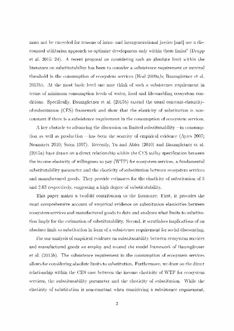
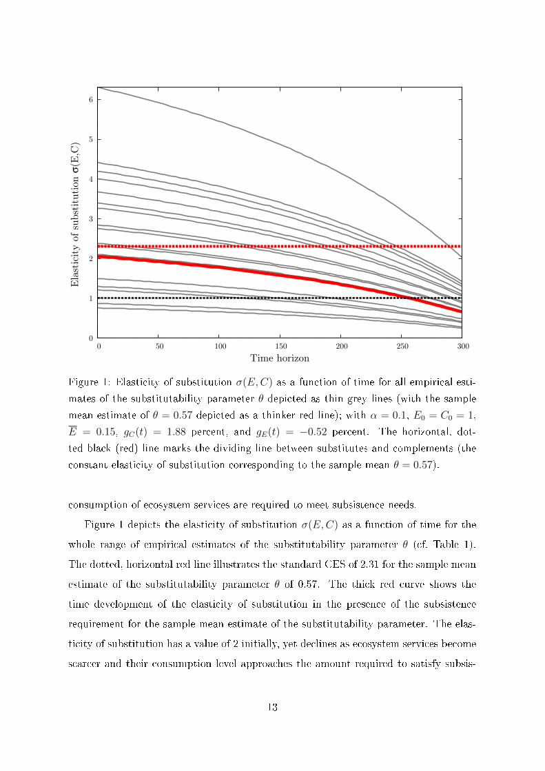
Figure 1: Elasticity of substitution σ(E,C) as a function of time for all empirical esti-

mates of the substitutability parameter θ depicted as thin grey lines (with the sample

mean estimate of θ = 0.57 depicted as a thinker red line); with α = 0.1, E0 = C0 = 1,

E = 0.15, gC(t) = 1.88 percent, and gE(t) = −0.52 percent. The horizontal, dot-

ted black (red) line marks the dividing line between substitutes and complements (the

constant elasticity of substitution corresponding to the sample mean θ = 0.57).

consumption of ecosystem services are required to meet subsistence needs.

Figure 1 depicts the elasticity of substitution σ(E,C) as a function of time for the

whole range of empirical estimates of the substitutability parameter θ (cf. Table 1).

The dotted, horizontal red line illustrates the standard CES of 2.31 for the sample mean

estimate of the substitutability parameter θ of 0.57. The thick red curve shows the

time development of the elasticity of substitution in the presence of the subsistence

requirement for the sample mean estimate of the substitutability parameter. The elas-

ticity of substitution has a value of 2 initially, yet declines as ecosystem services become

scarcer and their consumption level approaches the amount required to satisfy subsis-

13

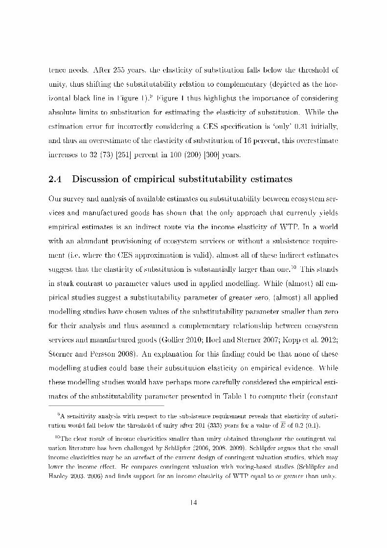
tence needs. After 255 years, the elasticity of substitution falls below the threshold of

unity, thus shifting the substitutability relation to complementary (depicted as the hor-

izontal black line in Figure 1).9 Figure 1 thus highlights the importance of considering

absolute limits to substitution for estimating the elasticity of substitution. While the

estimation error for incorrectly considering a CES speci�cation is `only' 0.31 initially,

and thus an overestimate of the elasticity of substitution of 16 percent, this overestimate

increases to 32 (73) [251] percent in 100 (200) [300] years.

2.4 Discussion of empirical substitutability estimates

Our survey and analysis of available estimates on substitutability between ecosystem ser-

vices and manufactured goods has shown that the only approach that currently yields

empirical estimates is an indirect route via the income elasticity of WTP. In a world

with an abundant provisioning of ecosystem services or without a subsistence require-

ment (i.e. where the CES approximation is valid), almost all of these indirect estimates

suggest that the elasticity of substitution is substantially larger than one.10 This stands

in stark contrast to parameter values used in applied modelling. While (almost) all em-

pirical studies suggest a substitutability parameter of greater zero, (almost) all applied

modelling studies have chosen values of the substitutability parameter smaller than zero

for their analysis and thus assumed a complementary relationship between ecosystem

services and manufactured goods (Gollier 2010; Hoel and Sterner 2007; Kopp et al. 2012;

Sterner and Persson 2008). An explanation for this �nding could be that none of these

modelling studies could base their substitution elasticity on empirical evidence. While

these modelling studies would have perhaps more carefully considered the empirical esti-

mates of the substitutability parameter presented in Table 1 to compute their (constant

9A sensitivity analysis with respect to the subsistence requirement reveals that elasticity of substi-

tution would fall below the threshold of unity after 201 (333) years for a value of E of 0.2 (0.1).

10The clear result of income elasticities smaller than unity obtained throughout the contingent val-

uation literature has been challenged by Schläpfer (2006, 2008, 2009). Schläpfer argues that the small

income elasticities may be an artefact of the current design of contingent valuation studies, which may

lower the income e�ect. He compares contingent valuation with voting-based studies (Schläpfer and

Hanley 2003, 2006) and �nds support for an income elasticity of WTP equal to or greater than unity.

14

approximation of the) elasticity of substitution, we hypothesise that they might not

and should not have simply settled with these estimates due to limiting biases of the

assumption of a normal, homogenous ecosystem service. Indeed, both a consideration

of heterogenous ecosystem services as well as their potential subsistence good nature

become relevant for putting the empirical estimates gathered into perspective.

First, our sample on the substitutability of ecosystem services is non-representative

of the true global distribution of ecosystem services. Valuation studies have been carried

out predominantly in developed countries and do not capture income e�ects on the whole

range of ecosystem services. In particular, valuation studies of climate- and disease

regulation as well as aesthetic and spiritual ecosystem services, which might have a low

degree of substitutability by manufactured goods, are often not accounted for.11

Second, even if information on the income elasticity of WTP were available for the

whole distribution of heterogenous ecosystem services, the non-trivial question of how

to aggregate these into a single ecosystem service good remains. In line with the previ-

ous literature, we assume that ecosystem services are a homogenous good and use the

unweighted arithmetic mean to aggregate substitutability of di�erent ecosystem services

with respect to manufactured goods. This implies that ecosystem services considered

are assumed to have the same weight and the elasticity of substitution with respect to

the manufactured good, or that there is perfect substitutability within the aggregate

ecosystem service. For example, we have given equal weight to the substitutability pa-

rameter derived from the single valuation study on recreation improvements (Whitehead

et al. 2000) as to the meta-studies on biodiversity conservation by Jacobsen and Hanley

(2009) or Lidhjem and Tuan (2012). Firstly, one might argue that meta-studies might

be weighted in relation to the single studies of our sample according to the number of

11While the omission of more di�cult to measure WTPs for ecosystem services might lead to an

overestimate of the overall degree of substitutability, the e�ect of an over-proportionate availability

of studies from developed countries might bias the estimate in the opposite direction. The available

evidence so far suggests that the income elasticity of WTP might be higher in high-income populations

(Barbier et al. 2015; Ready et al. 2002), suggesting that the current sample mean would underestimate

the average degree of substitutability. We cannot [can] con�rm this �nding when comparing developed

and developing countries for estimates derived from all [contingent] valuation studies in Table 1.

15

primary studies they contain. Secondly, one might argue, for example, that biodiver-

sity is more important for the aggregate state of ecosystem services than recreational

bene�ts and that it should be giver a greater weight. Furthermore, ecosystem services

will in general not have the same elasticity of substitution with respect to manufactured

goods, or be perfectly substitutable among each other.12 Regarding the implications

of heterogeneity of ecosystems services for substitutability of an aggregate ecosystem

service, it is worth quoting Sterner and Persson's (2008: 71) consideration of choosing a

low degree of substitutability for their analysis at length:

�[If ] there is a range of [ES] with di�erent elasticities of substitution, then the

relevant aggregate number is very likely not going to be the average of those elas-

ticities. It is the goods [...] with low elasticities that will dominate the calculation,

since these will be the ones with increasing shares in utility. This goes for clean

water, pollination services, and many other subtle aspects of the ecosystem that we

take for granted as long as they are plentiful.�

Finally, we have considered a suggestion by Heal (2009) and further developed in

Baumgärtner et al. (2015b) that the elasticity of substitution between ecosystem services

and manufactured goods is non-constant due to the existence of a subsistence require-

ment in the consumption of ecosystem services. Speci�cally, the elasticity of substitution

varies with the availability of ecosystem services in relation to the services necessary to

meet basic subsistence needs. Humans will not be willing to substitute ecosystem ser-

vices for manufactured goods if these subsistence requirements are not su�ciently met

and will be willing to substitute when ecosystem services are �plentiful�. This implies

that even if the aggregate ecosystem service is initially considered as a substitute, it will

� given a declining availability of ecosystem services � eventually become a complement

(see Figure 1). Even though the scenario analysis shows that the elasticity of substitu-

tion does not reach values of limited substitutability adopted in the applied modelling

literature (Sterner and Persson 2008) even for a time horizon of 300 years, it suggests

12Similar to measuring biodiversity (Bertram and Quaas 2016) one might consider an overall index

of ecosystem service abundance with imperfect substitutability among the single ecosystem services.

16

that the general notion of the concern addressed by the quote provided above may to a

considerable degree be resolved by considering absolute limits to substitution of ecosys-

tem services in the form of a subsistence requirement. More generally, it reconciles the

idea that mankind ultimately cannot, or is not willing to, live without the provisioning

of fundamental ecosystem services and the available empirical evidence suggesting that

the current willingness to substitute ecosystem services for manufactured goods still

seems to be high. This motivates exploring the implications of including an absolute

limit to substitution of ecosystem services in the form of a subsistence requirement for

intertemporal decision-making and social discounting.

3 Dual discounting under a subsistence requirement

3.1 Model and de�nitions

This section develops a dual discounting model that considers a subsistence requirement

in the consumption of ecosystem services. Our modelling set-up extends the approaches

of Hoel and Sterner (2007) and Traeger (2011): A social planner has perfect knowledge

about the future and maximizes an intertemporal, constant intertemporal elasticity

of substitution (CIES) social welfare function based on the CES instantaneous utility

function Uh (from Equation 2). Welfare is given by

W =

∫ T

0

1

1− η[α(Et − E)θ + (1− α)Cθ

t

] 1−ηθ︸ ︷︷ ︸

u(E,C)

e−δt

︸ ︷︷ ︸U(E,C,t)

dt, (5)

where δ is the utility discount rate and η is the inverse of the CIES with respect to

the within-period aggregate consumption bundle C =[α(Et − E)θ + (1− α)Cθ

t

] 1θ . We

assume a �nite time horizon T , due to the possibility of Et < E, implying that intertem-

poral welfare would be unde�ned.

Social discount factors and -rates are de�ned as follows (cf. Traeger 2011: 216): The

good-speci�c discount factors for good xi, with xi, xj ∈ {Et, Ct} and i 6= j, relating the

additional value of good xi between the points in time t and t0 for a given, but not

17

necessarily optimal, consumption path of E and C are

Pi(t, t0) =

∂U(Et,Ct,t)∂xi

∂U(Et,Ct,t0)∂xi

. (6)

The corresponding good-speci�c discount rates for good i are given by:

ρi(t) = −∂2U∂t∂xi

(t) + ∂2U∂2xi

(t)xi(t) + ∂2U∂xj∂xi

(t)xj(t)

∂U∂xi

(t). (7)

Using U(E,C, t) from Equation (5), this can be expressed in simpler terms as:

ρE(t) = δ + ψEEgE(t) + ψECgC(t) (8)

and

ρC(t) = δ + ψCCgC(t) + ψCEgE(t), (9)

where ψEE (resp. ψCC) is the elasticity of marginal utility of consumption of the aggre-

gate ecosystem service (resp. manufactured good) with respect to the ecosystem service

(manufactured good), and ψEC(ψCE) is the elasticity of marginal utility of consumption

of the ecosystem service (manufactured good) with respect to the manufactured good

(ecosystem service); The growth rates gi are de�ned as gi(t) = xi(t)xi(t)

.

3.2 Results

We now derive and analyse the good-speci�c discount rates and in particular their

di�erence � also termed `relative price e�ect' (Hoel and Sterner 2007) � in the presence

of a subsistence requirement in the consumption of ecosystem services (Appendix A.2).

The discount rate for ecosystem services is given by:

ρE(t) = δ+Et

Et − Eαη(Et − E)θ + (1− α)(1− θ)Cθ

t

α(Et − E)θ + (1− α)Cθt

gE(t)+(1− α)Cθ

t (η − (1− θ))α(Et − E)θ + (1− α)Cθ

t

gC(t)

(10)

while the manufactured good discount rates is given by

ρC(t) = δ+α(1− θ)(Et − E)θ + (1− α)ηCθ

t

α(Et − E)θ + (1− α)Cθt

gC(t) +αEt(Et − E)θ−1(η − (1− θ))α(Et − E)θ + (1− α)Cθ

t

gE(t) .

(11)

18

Deriving the di�erence in good-speci�c discount rates yields the `relative price e�ect':

∆ρ(t) = ρC(t)− ρE(t) = (1− θ)[gC(t)− Et

Et − EgE(t)

]. (12)

In the following, we analyse and illustrate the properties of the relative price e�ect only.

For the special case of E = 0, the relative price e�ect ∆ρ collapses to the formula

of the standard CES case ∆ρCES = (1 − θ) × [gC(t)− gE(t)]. If a positive amount of

ecosystem services is necessary for subsistence (E > 0), the relative price e�ect not only

depends on the substitutability parameter and the di�erence in the two good-speci�c

growth rates, but also on the consumption of ecosystem services over and above the sub-

sistence requirement. This ampli�es the e�ect of the growth rate of ecosystem services

on the relative price e�ect. For the relevant case of imperfect substitutes (θ < 1) and a

subsistence requirement (E > 0), we derive the following results from Equation (12):

Proposition 1

For Et > E > 0, bounded growth rates, and θ < 1, the `relative price e�ect' ∆ρ has the

following properties:

∂∆ρ(t)

∂ET 0 for gE(t) S 0 (13)

∂∆ρ(t)

∂θT 0 for gE(t)

Et

Et − ET gC(t) (14)

˙∆ρ(t) > 0 for ˙gC(t) = ˙gE(t) = 0 and gE(t) 6= 0 (15)

∆ρ(t) → ∞ for gE(t) < 0 (16)

∆ρ(t) → ∆ρCES for

gE(t) > 0

E → 0(17)

∆ρ T ∆ρCES for gE(t) S 0. (18)

Proof. See Appendix A.3.

Equation (13) states that the relative price e�ect increases (decreases) with the

stringency of the subsistence requirement if the growth rate of ecosystem services is

19

smaller (larger) than zero for all times. For the empirically relevant case of a decline in

ecosystem services, the relative price e�ect would therefore increase if a larger share of

ecosystem services would be necessary to meet subsistence needs.

Equation (14) shows that the e�ect of an increase of the substitutability parameter

depends on the relative magnitude of the growth rate for manufactured goods and the

growth rate for ecosystem services, weighted by their consumption relative to the amount

consumed over and above the subsistence requirement. As EtEt−E

> 1 for Et > E > 0,

the presence of the subsistence requirement reduces the parameter value space for which

an increase of the substitutability parameter will lead to a lower relative price e�ect.

Equation (15) shows that if the growth rates are constant (see, e.g., Baumgärtner et

al. 2015a; Hoel and Sterner 2007), and the growth rate of ecosystem services is di�erent

from zero, then the relative price e�ect will increase over time.

If ecosystem services are limited, the relative price e�ect is non-constant and de-

pends on the consumption of ecosystem services relative to the subsistence requirement.

Speci�cally, if ecosystem services are in a continuous decline, the relative price e�ect

increases and approaches in�nity in the limit (Equation 16). Equation (17) shows, in

contrast, that if the provisioning of ecosystem services grows over time and becomes

`plentiful', the relative price e�ect becomes equivalent to the standard CES case, as it

does for a vanishing subsistence requirement.

Equation (18) states that the relative price e�ect is larger (smaller) than its CES

version if the growth rate of ecosystem services is negative (positive). Naturally, for the

case of a constant consumption of ecosystem services, the two versions coincide and only

depend on the substitutability parameter and the growth rate of manufactured goods.

3.3 Empirical Analysis

We now illustrate the time development of the relative price e�ect of ecosystem services

under di�erent assumptions on substitutability and limits to substitution. We consider

the same scenario that we adopted in the analysis of the elasticity of substitution (Sec-

tion 2.3). The baseline parameters are taken from the 300-year simulation exercise of

Hoel and Sterner (2007), now including the social rate of pure time preference δ of 1

20

percent and a measure of intertemporal inequality aversion in consumption η of 1.5.

First, we estimate the relative price e�ects of ecosystem services ∆ρ corresponding to

each of the empirical estimates of the substitutability parameter θ. As the relative price

e�ect is non-constant due to the subsistence requirement and a decreasing availability

of ecosystem services, we compute it for three di�erent points in time: t = 0, 150

and 300 years (cf. Table 2, which also reports the relative price e�ect for prominent

assumptions in the dual discounting literature). Where possible, we also compute the

initial error range for the relative price e�ect.13 For the sample mean of empirical

estimates of the substitutability parameter we observe that the initial relative price

e�ect is 1.08 percentage-points and rises up to 1.15 (1.61) percentage-points in 150 (300)

years. For the smallest empirical estimate of the substitutability parameter (derived

from Barton 2002), the relative price e�ect is only 0.35 percentage-points initially and

rises to 0.52 percentage-points in 300 years. However, for the value derived from the

revealed preference study on air quality improvement in Italy (Martini and Tiezzi 2014),

the relative price e�ect is 2.89 percentage-points initially and rises up to 3.08 (4.31)

percentage-points in 150 (300) years.

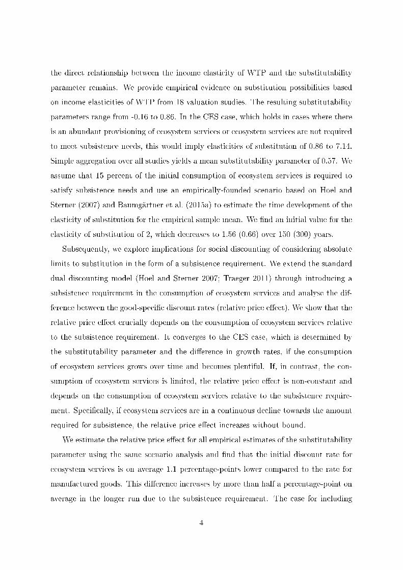
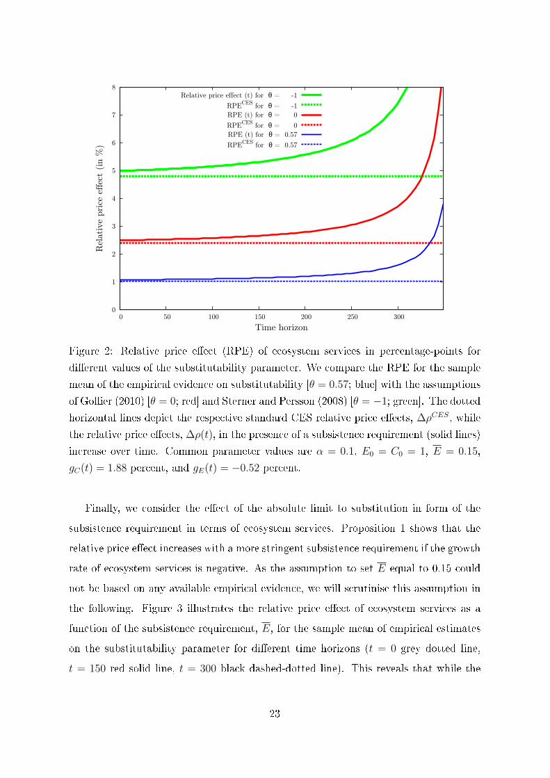
Second, we contrast the sample mean of empirical evidence on the substitutabil-

ity parameter with prominent assumptions from the literature (Gollier 2010; Sterner

and Persson 2010). Figure 2 depicts the relative price e�ect ∆ρ for these three cases

of the substitutability parameter θ and contrasts this with the constant relative price

e�ect ∆ρCES prevalent in the previous literature. The three cases represent initial

high (θ = 0.57), Cobb-Douglas (θ = 0) and limited substitutability (θ = −1). The

relative price e�ect in the presence of the subsistence requirement is always higher

than under the standard CES non-subsistence case for our parameter speci�cations,

i.e. gE(t) < 0 < gC(t), and increases without bound as we approach the subsistence

requirement in terms of ecosystem services.14 Over time, the relative price e�ect with

subsistence consumption rises considerably above its CES counterpart. For the limited

13The error range for the sample mean is computed as the standard deviation of the single initial

relative price e�ect estimates.

14With the given speci�cations, we approach the subsistence requirement after 363 years.

21

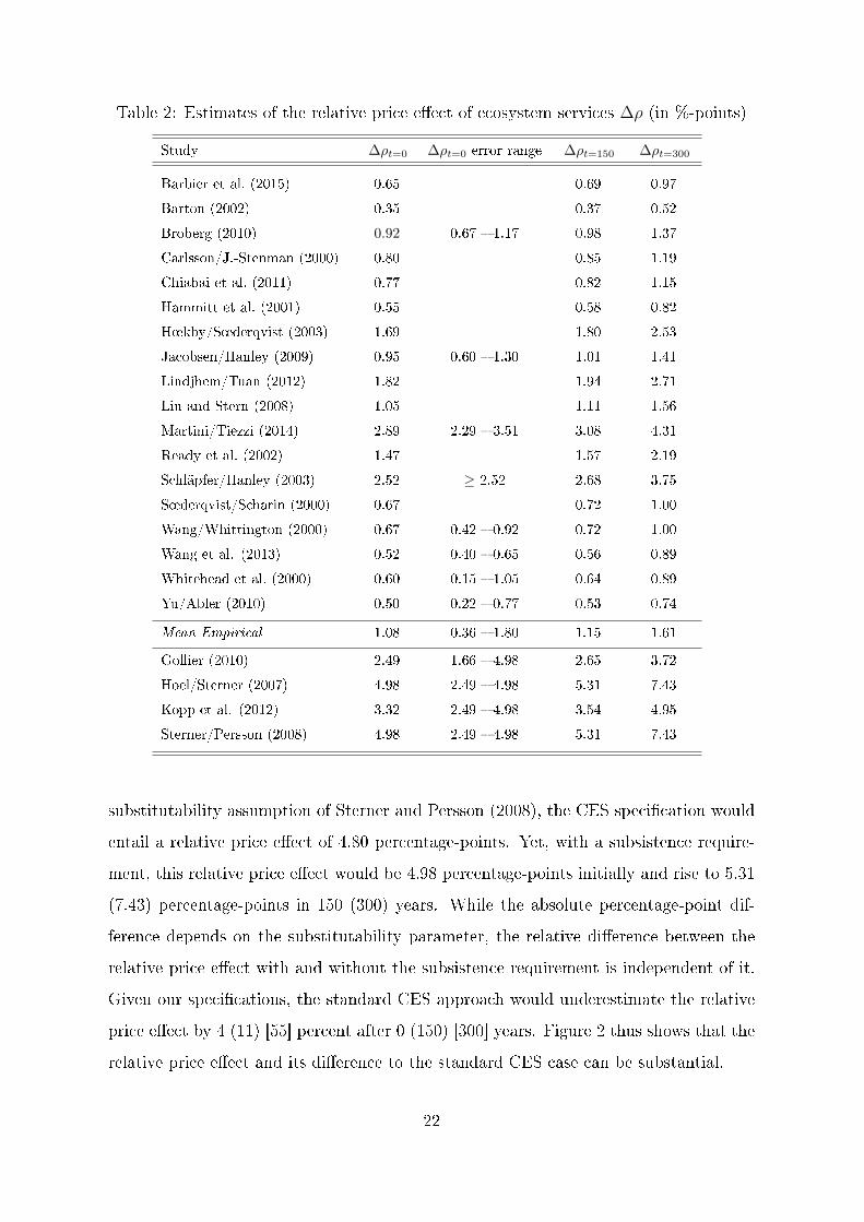
Table 2: Estimates of the relative price e�ect of ecosystem services ∆ρ (in %-points)

Study ∆ρt=0 ∆ρt=0 error range ∆ρt=150 ∆ρt=300

Barbier et al. (2015) 0.65 0.69 0.97

Barton (2002) 0.35 0.37 0.52

Broberg (2010) 0.92 0.67 � 1.17 0.98 1.37

Carlsson/J.-Stenman (2000) 0.80 0.85 1.19

Chiabai et al. (2011) 0.77 0.82 1.15

Hammitt et al. (2001) 0.55 0.58 0.82

H÷kby/S÷derqvist (2003) 1.69 1.80 2.53

Jacobsen/Hanley (2009) 0.95 0.60 � 1.30 1.01 1.41

Lindjhem/Tuan (2012) 1.82 1.94 2.71

Liu and Stern (2008) 1.05 1.11 1.56

Martini/Tiezzi (2014) 2.89 2.29 � 3.51 3.08 4.31

Ready et al. (2002) 1.47 1.57 2.19

Schläpfer/Hanley (2003) 2.52 ≥ 2.52 2.68 3.75

S÷derqvist/Scharin (2000) 0.67 0.72 1.00

Wang/Whittington (2000) 0.67 0.42 � 0.92 0.72 1.00

Wang et al. (2013) 0.52 0.40 � 0.65 0.56 0.89

Whitehead et al. (2000) 0.60 0.15 � 1.05 0.64 0.89

Yu/Abler (2010) 0.50 0.22 � 0.77 0.53 0.74

Mean Empirical 1.08 0.36 � 1.80 1.15 1.61

Gollier (2010) 2.49 1.66 � 4.98 2.65 3.72

Hoel/Sterner (2007) 4.98 2.49 � 4.98 5.31 7.43

Kopp et al. (2012) 3.32 2.49 � 4.98 3.54 4.95

Sterner/Persson (2008) 4.98 2.49 � 4.98 5.31 7.43

substitutability assumption of Sterner and Persson (2008), the CES speci�cation would

entail a relative price e�ect of 4.80 percentage-points. Yet, with a subsistence require-

ment, this relative price e�ect would be 4.98 percentage-points initially and rise to 5.31

(7.43) percentage-points in 150 (300) years. While the absolute percentage-point dif-

ference depends on the substitutability parameter, the relative di�erence between the

relative price e�ect with and without the subsistence requirement is independent of it.

Given our speci�cations, the standard CES approach would underestimate the relative

price e�ect by 4 (11) [55] percent after 0 (150) [300] years. Figure 2 thus shows that the

relative price e�ect and its di�erence to the standard CES case can be substantial.

22

0

1

2

3

4

5

6

7

8

0 50 100 150 200 250 300

Rel

ativ

e pri

ce e

ffec

t (in %

)

Time horizon

Relative price effect (t) for θ = -1

RPECES for θ = -1

RPE (t) for θ = 0

RPECES for θ = 0

RPE (t) for θ = 0.57

RPECES for θ = 0.57

Figure 2: Relative price e�ect (RPE) of ecosystem services in percentage-points for

di�erent values of the substitutability parameter. We compare the RPE for the sample

mean of the empirical evidence on substitutability [θ = 0.57; blue] with the assumptions

of Gollier (2010) [θ = 0; red] and Sterner and Persson (2008) [θ = −1; green]. The dotted

horizontal lines depict the respective standard CES relative price e�ects, ∆ρCES, while

the relative price e�ects, ∆ρ(t), in the presence of a subsistence requirement (solid lines)

increase over time. Common parameter values are α = 0.1, E0 = C0 = 1, E = 0.15,

gC(t) = 1.88 percent, and gE(t) = −0.52 percent.

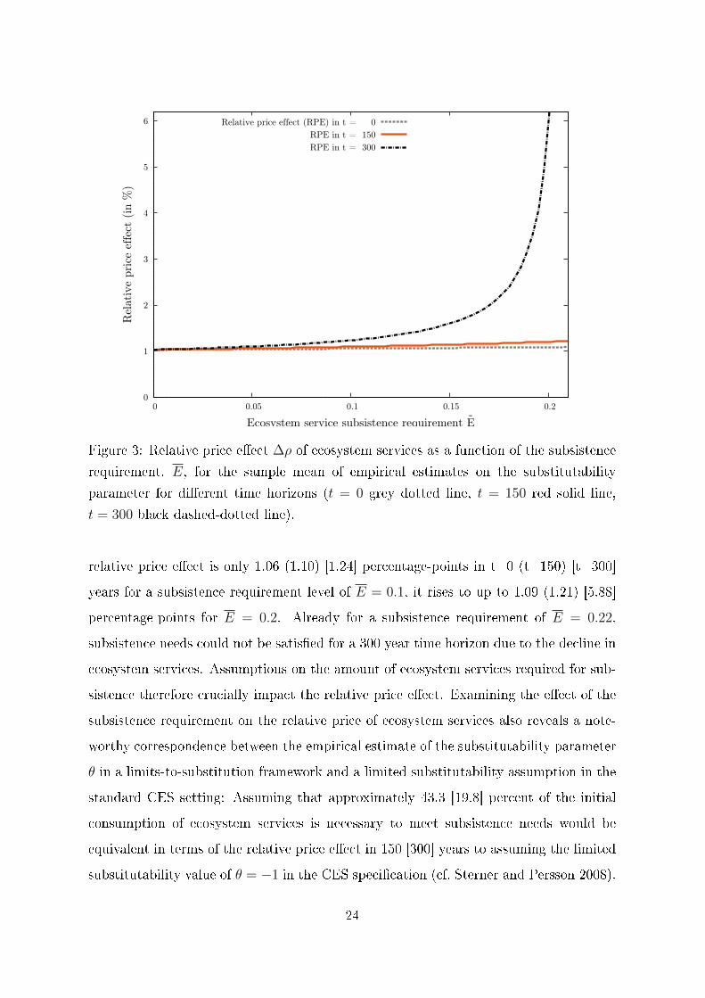
Finally, we consider the e�ect of the absolute limit to substitution in form of the

subsistence requirement in terms of ecosystem services. Proposition 1 shows that the

relative price e�ect increases with a more stringent subsistence requirement if the growth

rate of ecosystem services is negative. As the assumption to set E equal to 0.15 could

not be based on any available empirical evidence, we will scrutinise this assumption in

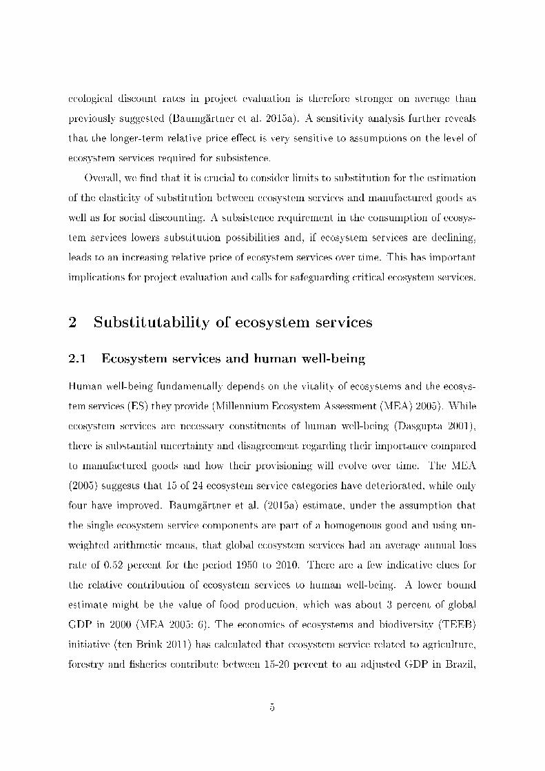
the following. Figure 3 illustrates the relative price e�ect of ecosystem services as a

function of the subsistence requirement, E, for the sample mean of empirical estimates

on the substitutability parameter for di�erent time horizons (t = 0 grey dotted line,

t = 150 red solid line, t = 300 black dashed-dotted line). This reveals that while the

23

0

1

2

3

4

5

6

0 0.05 0.1 0.15 0.2

Rel

ativ

e pri

ce e

ffec

t (in %

)

Ecosystem service subsistence requirement E-

Relative price effect (RPE) in t = 0

RPE in t = 150

RPE in t = 300

Figure 3: Relative price e�ect ∆ρ of ecosystem services as a function of the subsistence

requirement, E, for the sample mean of empirical estimates on the substitutability

parameter for di�erent time horizons (t = 0 grey dotted line, t = 150 red solid line,

t = 300 black dashed-dotted line).

relative price e�ect is only 1.06 (1.10) [1.24] percentage-points in t=0 (t=150) [t=300]

years for a subsistence requirement level of E = 0.1, it rises to up to 1.09 (1.21) [5.88]

percentage-points for E = 0.2. Already for a subsistence requirement of E = 0.22,

subsistence needs could not be satis�ed for a 300 year time horizon due to the decline in

ecosystem services. Assumptions on the amount of ecosystem services required for sub-

sistence therefore crucially impact the relative price e�ect. Examining the e�ect of the

subsistence requirement on the relative price of ecosystem services also reveals a note-

worthy correspondence between the empirical estimate of the substitutability parameter

θ in a limits-to-substitution framework and a limited substitutability assumption in the

standard CES setting: Assuming that approximately 43.3 [19.8] percent of the initial

consumption of ecosystem services is necessary to meet subsistence needs would be

equivalent in terms of the relative price e�ect in 150 [300] years to assuming the limited

substitutability value of θ = −1 in the CES speci�cation (cf. Sterner and Persson 2008).

24

4 Conclusions

This paper has examined implications of an absolute limit to substitution of ecosystem

services on estimating substitutability between ecosystem services and manufactured

consumption goods as well as on the theory and empirics of social discounting of ecosys-

tem services. Speci�cally, we have considered a case where substitution possibilities are

restricted by a subsistence requirement in the consumption of ecosystem services, which

may consist of water, food and life-enabling ecosystem conditions.

Based on a framework that allows for absolute limits to substitution, we provide

empirical estimates of the substitutability of ecosystem services. In the standard con-

stant elasticity of substitution (CES) case discussed in the literature (Baumgärtner et

al. 2015a; Yu and Abler 2010), there is a direct relationship between the income elas-

ticity of WTP for ecosystem services, a fundamental substitutability parameter and the

CES. If there is a subsistence requirement, this direct relationship between the elasticity

of substitution and the other two breaks down. We provide a comprehensive account

of empirical estimates on the substitutability parameter and, by means of a long-term

simulation, analyse what these may imply for estimating the elasticity of substitution.

We �nd that empirical evidence on the substitutability parameter suggests that

most ecosystem services are considered highly substitutable by manufactured goods.

Assuming that individual services are part of a homogenous ecosystem service good,

we aggregate over all studies and �nd a mean substitutability parameter of 0.57. The

scenario analysis reveals that the elasticity of substitution for the sample mean has a

value of 2 initially and decreases to 1.56 (0.66) over 150 (300) years. Compared to this

variable elasticity of substitution, the CES approach would result in an estimation error

of 32 (73) percent after 100 (200) years. Substitution possibilities are thus considerably

lower as previously suggested (Yu and Abler 2010; Baumgärtner et al. 2015a).

Subsequently, we explore implications of considering an absolute limit to substitution

for social discounting, by extending dual discounting models to allow for a subsistence

requirement in the consumption of ecosystem services. We �nd that the relative price

e�ect of ecosystem services not only depends on the substitutability parameter and the

25

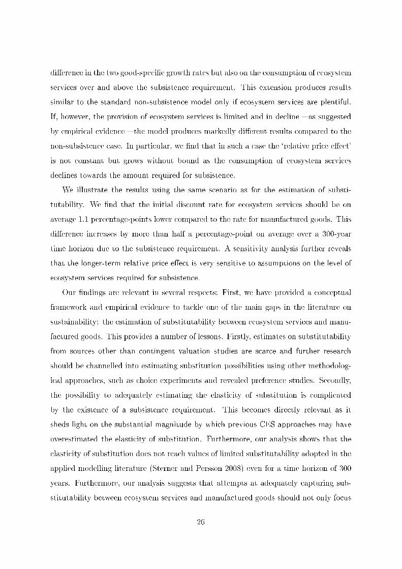
di�erence in the two good-speci�c growth rates but also on the consumption of ecosystem

services over and above the subsistence requirement. This extension produces results

similar to the standard non-subsistence model only if ecosystem services are plentiful.

If, however, the provision of ecosystem services is limited and in decline � as suggested

by empirical evidence � the model produces markedly di�erent results compared to the

non-subsistence case. In particular, we �nd that in such a case the `relative price e�ect'

is not constant but grows without bound as the consumption of ecosystem services

declines towards the amount required for subsistence.

We illustrate the results using the same scenario as for the estimation of substi-

tutability. We �nd that the initial discount rate for ecosystem services should be on

average 1.1 percentage-points lower compared to the rate for manufactured goods. This

di�erence increases by more than half a percentage-point on average over a 300-year

time horizon due to the subsistence requirement. A sensitivity analysis further reveals

that the longer-term relative price e�ect is very sensitive to assumptions on the level of

ecosystem services required for subsistence.

Our �ndings are relevant in several respects: First, we have provided a conceptual

framework and empirical evidence to tackle one of the main gaps in the literature on

sustainability: the estimation of substitutability between ecosystem services and manu-

factured goods. This provides a number of lessons. Firstly, estimates on substitutability

from sources other than contingent valuation studies are scarce and further research

should be channelled into estimating substitution possibilities using other methodolog-

ical approaches, such as choice experiments and revealed preference studies. Secondly,

the possibility to adequately estimating the elasticity of substitution is complicated

by the existence of a subsistence requirement. This becomes directly relevant as it

sheds light on the substantial magnitude by which previous CES approaches may have

overestimated the elasticity of substitution. Furthermore, our analysis shows that the

elasticity of substitution does not reach values of limited substitutability adopted in the

applied modelling literature (Sterner and Persson 2008) even for a time horizon of 300

years. Furthermore, our analysis suggests that attempts at adequately capturing sub-

stitutability between ecosystem services and manufactured goods should not only focus

26

on methodological approaches other than contingent valuation studies, but in particular

that one would need to perform long-term studies that scrutinise how estimates of the

elasticity of substitution develop over time and which factors in�uence it. Lastly, the

substantial heterogeneity of indirect estimates on substitutability of ecosystem services

that we obtained � across as well as within di�erent ecosystem services categories � ques-

tions the often adopted assumptions of a homogenous ecosystem service good. Future

research should therefore explore implications of this heterogeneity.

Second, our results provide stronger support for the case of including ecological

discount rates in project evaluation (Baumgärtner et al. 2015a). We �nd that ecosystem

services should be discounted at a rate that is 1.1 percentage points lower than the rate

for manufactured consumption goods initially and 1.6 percentage points for a 300-year

time horizon. Indeed, none of our estimates suggests that ecosystem services should be

discounted at the same rate as manufactured goods.

Finally, this paper relates to the intensely debated notions of `planetary boundaries'

(Rockström et al. 2009) and `catastrophic' climate change (Millner 2013; Weitzman

2009). By emphasising the importance of basic subsistence needs, our approach re-

connects the study of intertemporal allocation to the original notion of sustainability

(WCED 1987). Furthermore, in our setting, `catastrophic' climate change might be

conceptualised as the loss of ecosystem services required for subsistence, such as an ad-

equate food supply, fresh water, and life-enabling ecosystem conditions. This does not

imply that a focus on fat-tailed probability distributions of climate damages is super-

�uous � indeed these `dismal' results would be even more `dismal' if catastrophe occurs

already at a strictly positive consumption level. But it follows that more e�ort should be

channelled into discussing the substance of the notion of `catastrophe' and that climate

policies should aim �rst and foremost at secures the provisioning of subsistence services.

Our analysis has shown that the relative price e�ect of ecosystem services is very sensi-

tive to the amount of ecosystem services required for subsistence. More research, as well

as societal and political discussions, should therefore be channelled into determining the

magnitude and composition of such a subsistence requirement.

27

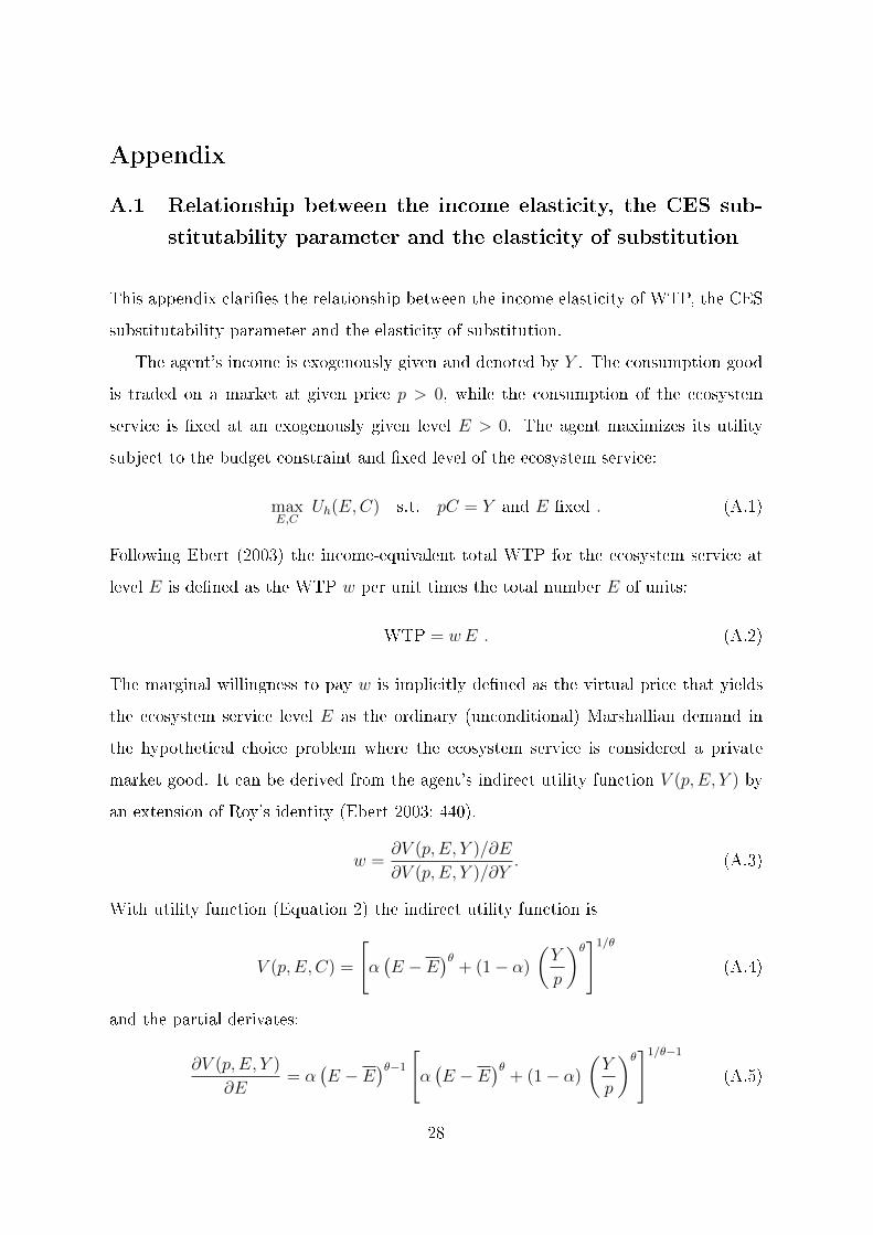
Appendix

A.1 Relationship between the income elasticity, the CES sub-

stitutability parameter and the elasticity of substitution

This appendix clari�es the relationship between the income elasticity of WTP, the CES

substitutability parameter and the elasticity of substitution.

The agent's income is exogenously given and denoted by Y . The consumption good

is traded on a market at given price p > 0, while the consumption of the ecosystem

service is �xed at an exogenously given level E > 0. The agent maximizes its utility

subject to the budget constraint and �xed level of the ecosystem service:

maxE,C

Uh(E,C) s.t. pC = Y and E �xed . (A.1)

Following Ebert (2003) the income-equivalent total WTP for the ecosystem service at

level E is de�ned as the WTP w per unit times the total number E of units:

WTP = wE . (A.2)

The marginal willingness to pay w is implicitly de�ned as the virtual price that yields

the ecosystem service level E as the ordinary (unconditional) Marshallian demand in

the hypothetical choice problem where the ecosystem service is considered a private

market good. It can be derived from the agent's indirect utility function V (p, E, Y ) by

an extension of Roy's identity (Ebert 2003: 440).

w =∂V (p, E, Y )/∂E

∂V (p, E, Y )/∂Y. (A.3)

With utility function (Equation 2) the indirect utility function is

V (p, E, C) =

[α(E − E

)θ+ (1− α)

(Y

p

)θ]1/θ(A.4)

and the partial derivates:

∂V (p, E, Y )

∂E= α

(E − E

)θ−1 [α(E − E

)θ+ (1− α)

(Y

p

)θ]1/θ−1(A.5)

28

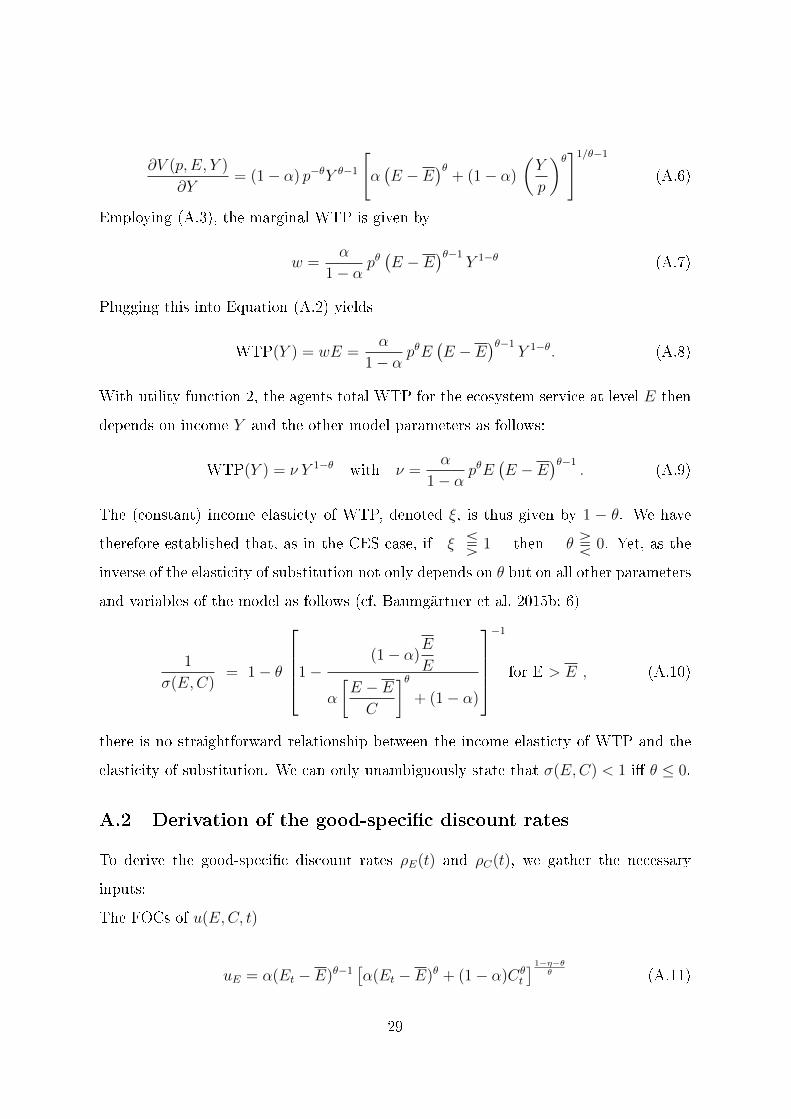
∂V (p, E, Y )

∂Y= (1− α) p−θY θ−1

[α(E − E

)θ+ (1− α)

(Y

p

)θ]1/θ−1(A.6)

Employing (A.3), the marginal WTP is given by

w =α

1− αpθ(E − E

)θ−1Y 1−θ (A.7)

Plugging this into Equation (A.2) yields

WTP(Y ) = wE =α

1− αpθE

(E − E

)θ−1Y 1−θ. (A.8)

With utility function 2, the agents total WTP for the ecosystem service at level E then

depends on income Y and the other model parameters as follows:

WTP(Y ) = ν Y 1−θ with ν =α

1− αpθE

(E − E

)θ−1. (A.9)

The (constant) income elasticty of WTP, denoted ξ, is thus given by 1 − θ. We have

therefore established that, as in the CES case, if ξ S 1 then θ T 0. Yet, as the

inverse of the elasticity of substitution not only depends on θ but on all other parameters

and variables of the model as follows (cf. Baumgärtner et al. 2015b: 6)

1

σ(E,C)= 1− θ

1−(1− α)

E

E

α

[E − EC

]θ+ (1− α)

−1

for E > E , (A.10)

there is no straightforward relationship between the income elasticty of WTP and the

elasticity of substitution. We can only unambiguously state that σ(E,C) < 1 i� θ ≤ 0.

A.2 Derivation of the good-speci�c discount rates

To derive the good-speci�c discount rates ρE(t) and ρC(t), we gather the necessary

inputs:

The FOCs of u(E,C, t)

uE = α(Et − E)θ−1[α(Et − E)θ + (1− α)Cθ

t

] 1−η−θθ (A.11)

29

uC = (1− α)Cθ−1t

[α(Et − E)θ + (1− α)Cθ

t

] 1−η−θθ (A.12)

and SOCs

uEE = −α(Et−E)θ−2 (αη(Et−E)θ +(1−θ)(1−α)Cθt )[α(Et − E)θ + (1− α)Cθ

t

] 1−η−2θθ

(A.13)

uCC = −(1− α)Cθ−2t (α(1− θ)(Et−E)θ + η(1− α)Cθ

t )[α(Et − E)θ + (1− α)Cθ

t

] 1−η−2θθ

(A.14)

uEC = uCE = (1− α)αCθ−1t (Et − E)θ−1(1− η − θ)

[α(Et − E)θ + (1− α)Cθ

t

] 1−η−2θθ

(A.15)

are used to derive the respective elasticities of marginal utility

ψEE := −uEE(·)EtuE(·)

=Et

Et − E

[αη(E − E)θ + (1− α)(1− θ)Cθ

t

α(Et − E)θ + (1− α)Cθt

](A.16)

ψCC := −uCC(·)CtuC(·)

=α(1− θ)(E − E)θ + (1− α)ηCθ

t

α(Et − E)θ + (1− α)Cθt

(A.17)

ψEC := −uEC(·)CtuE(·)

=(1− α)Cθ

t (η + θ − 1)

α(Et − E)θ + (1− α)Cθt

(A.18)

ψCE := −uCE(·)EtuC(·)

=αE(E − E)θ−1(η + θ − 1)

α(Et − E)θ + (1− α)Cθt

. (A.19)

Using these, the good-speci�c discount rates are given by (cf. Equations (8) and (9)):

ρE(t) = δ+Et

Et − Eαη(E − E)θ + (1− α)(1− θ)Cθ

t

α(Et − E)θ + (1− α)Cθt

gE(t)+(1− α)Cθ

t (η − (1− θ))α(Et − E)θ + (1− α)Cθ

t

gC(t)

(A.20)

30

and

ρC(t) = δ +α(1− θ)(E − E)θ + (1− α)ηCθ

t

α(Et − E)θ + (1− α)Cθt

gC(t) +αE(E − E)θ−1(η − (1− θ))α(Et − E)θ + (1− α)Cθ

t

gE(t) .

(A.21)

A.3 Proof of Proposition 1

We now derive the properties of the relative price e�ect, ∆ρ(t) = (1−θ)[gC(t)− Et

Et−EgE(t)

]for Et > E > 0 and θ < 1, as presented in Proposition 1:

Equation (13):

∂∆ρ(t)

∂E= −(1− θ) gE(t)Et

(Et − E)2T 0 for gE(t) S 0 (A.22)

Equation (14):

∂∆ρ(t)

∂θ= gE(t)

Et

Et − E− gC(t) T 0 for gE(t)

Et

Et − ET gC(t) (A.23)

Equations (17) and (16):

˙∆ρ(t) = (1− θ)

[˙gC(t)− ˙gE(t)

Et

Et − E+gE(t)EtE

(Et − E)2

]

= (1− θ)

[˙gC(t)− ˙gE(t)

Et

Et − E+gE(t)2EtE

(Et − E)2

]. (A.24)

For the special case of ˙gC(t) = ˙gE(t) = 0 and gE(t) 6= 0, we obtain for Equation (15):

˙∆ρ(t) =gE(t)EtE

(Et − E)2=

gE(t)2EtE

(Et − E)2> 0 . (A.25)

For gE(t) > 0, Et →∞ as t→∞. Therefore, we obtain for Equation (17):

limEt→∞

˙∆ρ(t) = (1− θ)[

˙gC(t)− ˙gE(t)]

= ∆ρCES(t) . (A.26)

For gE(t) < 0, and bounded (changes in) growth rates, Et → E in �nite t. Therefore,

we obtain for Equation (16):

limEt→E

˙∆ρ(t) =∞ . (A.27)

31

References

Ayres, R.U. (2007), On the practical limits to substitution, Ecological Economics 61(1):

115�128.

Barbier, E.B., M. Czajkowski and N. Hanley (2015), Is the income elasticity of the will-

ingness to pay for pollution control constant? University of St. Andrews, Department

of Geography and Sustainable Development Working Paper No 2015-04.

Barton, D. N. (2002), The transferability of bene�t transfer: contingent valuation of

water quality improvements in Costa Rica, Ecological Economics 42(1): 147�164.

Baumgärtner, S., A.-M. Klein, D. Thiel and K. Winkler (2015a), Ramsey Discounting

of Ecosystem Services, Environmental and Resource Economics 61: 273�296.

Baumgärtner, S., M.A. Drupp and M.F. Quaas (2015b), Subsistence, substitutability

and sustainability in consumer preferences, forthcoming in Environmental and Re-

source Economics, available at: http://link.springer.com/article/10.1007%2Fs10640-

015-9976-z.

Baumgärtner, S., M.A. Drupp, J. Meya, M. Munz and M.F. Quaas (2016), Income

Inequality and Willingness to Pay for Public Environmental Goods, University of

Kiel Economics Working Paper 2016-04.

Bertram C., and M.F. Quaas (2016), Biodiversity and Optimal Multi-species Ecosystem

Management, forthcoming in Environmental and Resource Economics, available at:

http://link.springer.com/article/10.1007/s10640-015-9988-8.

Broberg, T. (2010), Income treatment e�ects in contingent valuation: the case of the

Swedish predator policy, Environmental and Resource Economics 46(1): 1�17.

Carlsson, F. and O. Johansson-Stenman (2000), Willingness to pay for improved air

quality in Sweden, Applied Economics 32: 661�669.

32

Chiabai, A., C. Travisi, A. Markandya, H. Ding and P. Nunes (2011), Economic assess-

ment of forest ecosystem services losses: cost of policy inaction, Environmental and

Resource Economics 50(3): 405�445.

Dasgupta, P. (2001), Human Well-Being and the Natural Environment, Oxford and New

York: Oxford University Press.

Dasgupta, P. (2010), Nature's role in sustaining economic development, Philosophical

Transactions of the Royal Society B: Biological Sciences 365(1537): 5�11.

Drupp, M.A., Freeman, M.C., Groom, B. and F. Nesje (2015), Discounting Disentangled,

Grantham Research Institute on Climate Change and the Environment Working Paper

No. 172.

Dupoux, M. and V. Martinet (2014), Context-dependent substitutability: impacts on

environmental preferences and discounting, paper presented at the 2014 WCERE

conference.

Ebert, U. (2003), Environmental goods and the distribution of income, Environmental

and Resource Economics 25(4): 435�459.

Ehrlich, P.R. (1989), The limits to substitution: Meta-resource depletion and a new

economic-ecological paradigm, Ecological Economics 1(1): 9�16.

Fenichel, E.P. and J. Zhao (2015), Sustainability and substitutability, Bulletin of

Mathematical Biology 77(2): 348�367.

Fitter, A.H. (2013), Are Ecosystem Services Replaceable by Technology?, Environmental

and Resource Economics 55(4): 513�524.

Gerlagh, R. and B. van der Zwaan (2002), Long-term substitutability between environ-

mental and man-made goods, Journal of Environmental Economics and Management

44: 329�345.

Gollier, C. (2010), Ecological discounting, Journal of Economic Theory 145: 812�829.

33

Guesnerie, R. (2004), Calcul economique et d'eveloppement durable, Revue E'conomique

55: 363�382.

Hammitt, J., J.-T. Liu and J.-L. Liu (2001), Contingent valuation of a Taiwanese

wetland, Environment and Development Economics 6: 259�268.

Hanemann, W.M. (1991), Willingness to pay and willingness to accept: how much can

they di�er?, American Economic Review 81(3): 635�647.

Heal, G. (2009a), The economics of climate change: a post-Stern perspective, Climatic

Change 96(3): 275�297.

Heal, G. (2009b), Climate Economics: A Meta-Review and Some Suggestions for Future

Research, Review of Environmental Economics and Policy 3(1): 4�21.

Hoel, M. and T. Sterner (2007), Discounting and relative prices, Climatic Change 84:

265�280.

H÷okby, S. and T. S÷derqvist (2003), Elasticities of demand and willingness to pay

for ecosystem services in Sweden, Environmental and Resource Economics 26(3):

361�383.

Horowitz, J.K. and K.E. McConnell (2003), Willingness to accept, willingness to pay

and the income e�ect, Journal of Economic Behavior & Organization 51(4): 537�545.

Jacobsen, J. and N. Hanley (2009), Are there income e�ects on global willingness to

pay for biodiversity conservation? Environmental and Resource Economics 43(2):

137�160.

Kopp, R.E., A. Golub, N.O. Keohane and C. Onda (2012), The In�uence of the Speci-

�cation of Climate Change Damages on the Social Cost of Carbon, Economics: The

Open-Access, Open- Assessment E-Journal 6.

Kovenock, D. and E. Sadka (1981), Progression under the bene�t approach to the theory

of taxation, Economics Letters 8: 95�99.

34

Kristr÷m, B. and P. Riera (1996), Is the income elasticity of environmental improve-

ments less than one? Environmental and Resource Economics 7: 45�55.

Lindhjem, H., and Tuan, T.H. (2012), Valuation of species and nature conservation

in Asia and Oceania: a meta-analysis, Environmental Economics and Policy Studies

14(1): 1�22.

Liu, S. and D.I. Stern (2008), A meta-analysis of contingent valuation studies in coastal

and bear-shore marine ecosystems, CSIRO Working Paper Series 2008-15.

Martini, C. and S. Tiezzi (2014), Is the environment a luxury? An empirical inves-

tigation using revealed preferences and household production, Resource and Energy

Economics 37: 147�167.

[MEA, 2005] Millennium Ecosystem Assessment (2005), Ecosystems and Human Well-

Being: Synthesis, Washington, DC: Island Press.

Millner, A. (2013), On welfare frameworks and catastrophic climate risks, Journal of

Environmental Economics and Management 65(2): 310�325.

Neumayer, E. (2007), A missed opportunity: the Stern Review on climate change fails

to tackle the issue of non-substitutable loss of natural capital, Global Environmental

Change 17: 297�201.

Neumayer, E. (2010), Weak Versus Strong Sustainability: Exploring the Limits of Two

Opposing Paradigms, Cheltenham, UK, Edward Elgar, 3rd Edition.

Pezzey, J.C.V. and J.M. Anderies (2003), The e�ect of subsistence on collapse and

institutional adaptation in population�resource societies, Journal of Development

Economics 72: 299�320.

Ready, R.C., J. Malzubris and S. Senkane (2002), The relationship between environ-

mental values and income in a transition economy: surface water quality in Latvia,

Environment and Development Economics 7(1): 147�156.

35

Revankar, N.S. (1971), A class of variable elasticity of substitution production functions,

Econometrica 39(1): 61�71.

Rockström, J. et al. (2009), A safe operating space for humanity, Nature 461: 472�475.

Schläpfer, F. and N. Hanley (2003), Do local landscape patterns a�ect the demand for

landscape amenities protection?, Journal of Agricultural Economics 54(1): 21�34.

Schläpfer, F. and N. Hanley (2006), Contingent valuation and collective choice, KYK-

LOS 59(1): 115�135.

Schläpfer, F. (2006), Survey protocol and income e�ects in the contingent valuation of

public goods: A meta-analysis, Ecological Economics 57(3): 415�429.

Schläpfer, F. (2008), Contingent valuation: a new perspective, Ecological Economics

64(4): 729�740.

Schläpfer, F. (2009), Contingent valuation: confusions, problems, and solutions, Eco-

logical Economics 68(6): 1569�1571.

Sharif, M. (1986), The Concept and Measurement of Subsistence: A Survey of the

Literature, World Development 14(5): 555�577.

S÷oderqvist, T. and H. Scharin (2000), The regional willingness to pay for a reduced

eutrophication in the Stockholm archipelago, Beijer Discussion Paper No. 128.

Steger, T.M. (2000), Economic growth with subsistence consumption, Journal of De-

velopment Economics 62(2): 343�361.

Stern, D.I. (1997), Limits to substitution and irreversibility in production and con-

sumption: a neoclassical interpretation of ecological economics, Ecological Economics

21(3): 197�215.

Stern, N. (2007), The Economics of Climate Change: The Stern Review, Cambridge,

UK: Cambridge University Press.

36

Sterner, T. and M. Persson (2008), An even sterner review: introducing relative prices

into the discounting debate, Review of Environmental Economics and Policy 2(1):

61�76.

Ten Brink, P. (Ed.) (2011), The Economics of Ecosystems and Biodiversity in National

and International Policy Making, London, Earthscan.

Traeger, C.P. (2011), Sustainability, limited substitutability, and non-constant social

discount rates, Journal of Environmental Economics and Management 62(2): 215�

228.

Wang, H. and D. Whittington (2000), Willingness to Pay for Air Quality Improvement

in So�a, Bulgaria, World Bank Policy Research Working Paper 2280, Washington

DC: The World Bank.

Wang, H., Y. Shi, Y. Kim and T. Kamata (2013), Valuing water quality improvement

in China. A case study of Lake Puzhehei in Yunnan Province, Ecological Economics

94: 56�65.

[WCED (1987)] World Commission on Environment and Development (1987). Our

Common Future, Oxford, Oxford University Press. Online at: http://www.un-

documents.net/ocf-02.htm.

Weikard, H.-P. and X. Zhu (2005), Discounting and environmental quality: when should

dual rates be used?, Economic Modelling 22: 868�878.

Weitzman, M.L. (2009), On modeling and interpreting the economics of catastrophic

climate change, Review of Economics and Statistics 91(1): 1�19.

Weitzman, M.L. (2010), What is the damages function for global warming and what

di�erence might it make?, Climate Change Economics 1(1): 57�69.

Whitehead, J.C., T.C. Haab and J.-C. Huang (2000), Measuring Recreation Bene�ts

of Quality Improvements with Revealed and Stated Behavior Data, Resource and

Energy Economics 22: 339�354

37

Yu, X. and D. Abler (2010), Incorporating zero and missing responses into CVM with

openended bidding: willingness to pay for blue skies in Beijing, Environmental and

Development Economics 15: 535�556.

38