Technische Universit at Graz

Challenges and Applications of Boundary ElementDomain Decomposition Methods

O. Steinbach

Berichte aus demInstitut fur Numerische Mathematik

Bericht 2006/9

Technische Universit at Graz

Challenges and Applications of Boundary ElementDomain Decomposition Methods

O. Steinbach

Berichte aus demInstitut fur Numerische Mathematik

Bericht 2006/9

Technische Universitat GrazInstitut fur Numerische MathematikSteyrergasse 30A 8010 Graz

WWW: http://www.numerik.math.tu-graz.at

c© Alle Rechte vorbehalten. Nachdruck nur mit Genehmigung des Autors.

Challenges and Applications of Boundary Element

Domain Decomposition Methods

Olaf Steinbach

Institute for Computational Mathematics, Graz University of Technology,Steyrergasse 30, 8010 Graz, Austria, o.steinbach@tugraz.at

Abstract

Boundary integral equation methods are well suited to represent the Dirichlet to Neumann

maps which are required in the formulation of domain decomposition methods. Based on the

symmetric representation of the local Steklov–Poincare operators by a symmetric Galerkin

boundary element method, we describe a stabilised variational formulation for the local Dirich-

let to Neumann map. By a strong coupling of the Neumann data across the interfaces, we

obtain a mixed variational formulation. For biorthogonal basis functions the resulting system

is equivalent to nonredundant finite and boundary element tearing and interconnecting meth-

ods. We will also address several open questions, ideas and challenging tasks in the numerical

analysis of boundary element domain decomposition methods, in the implementation of those

algorithms, and their applications.

1 Introduction

Boundary element methods are well established approximation methods to solve exterior boundaryvalue problems, or to solve partial differential equations with (piecewise) constant coefficientsconsidered in complicated substructures and in domains with moving boundaries. For an stateof the art overview on recent advances on mathematical aspects and engineering applications ofboundary integral equation methods, see, for example, Schanz and Steinbach [2007]. However,for partial differential equations with nonlinear coefficients the coupling of finite and boundaryelement methods seems to be an efficient tool to solve complex problems in complicated domains.For the formulation and for an efficient solution of the resulting systems of equations, domaindecomposition methods are mandatory.The classical approach to couple finite and boundary element methods is to use only the weaklysingular boundary integral equation with single and double layer potentials, see, e.g., Brezzi andJohnson [1979], Johnson and Nedelec [1980], and Wendland [1988]. In Costabel [1987] a symmetriccoupling of finite and boundary elements using the so–called hypersingular boundary integral op-erator was introduced. This approach was then extended to symmetric Galerkin boundary elementmethods, see, e.g., Hsiao and Wendland [1990]. Appropriate preconditioned iterative strategieswere later considered in Carstensen et al. [1998], while quite general preconditioners based onoperators of the opposite order were introduced in Steinbach and Wendland [1998]. Boundary ele-ment tearing and interconnecting (BETI) methods were described in Langer and Steinbach [2003]as counterpart of FETI methods while in Langer et al. [2006] these methods were combined with afast multipole approximation of the local boundary integral operators involved. For an alternativeapproach to boundary integral domain decomposition methods see also Khoromskij and Wittum[2004].Here we will give a quite general setting of tearing and interconnecting, or more general, hybriddomain decomposition methods. The local partial differential equation is rewritten as a localDirichlet to Neumann map which can be realized either by domain variational formulations orby using boundary integral formulations. Since the related function spaces are fractional Sobolevspaces, one may ask for the right definition of the associated norms. It turns out that the usednorms which are induced by the local single layer potential or its inverse allows for almost explicitespectral equivalence inequalities, and an appropriate stabilisation of the singular Steklov–Poincareoperators. The modified Dirichlet to Neumann map is then used to obtain a mixed variationalformulation allowing a weak coupling of the local Dirichlet data. However, staying with a globallyconform method and using biorthogonal basis functions we end up with the standard tearing andinterconnecting approach as in FETI and in BETI.

5

The aim of this paper is to sketch some ideas to obtain advanced formulations in boundary integraldomain decomposition methods, to propose to use special norms in the numerical analysis, and tostate some challenging tasks in the implementation of fast boundary element domain decompositionalgorithms to solve challenging problems from engineering and industry.

2 Boundary Integral Equation DD Methods

As a model problem we consider the Dirichlet boundary value problem of the potential equation,

−div[α(x)∇u(x)] = f(x) for x ∈ Ω, u(x) = g(x) for x ∈ Γ (1)

where Ω ⊂ R3 is a bounded domain with Lipschitz boundary Γ = ∂Ω. We assume that there is

given a non–overlapping domain decomposition

Ω =

p⋃

i=1

Ωi, Ωi ∩ Ωj = ∅ for i 6= j, Γi = ∂Ωi. (2)

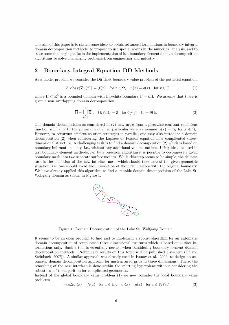
The domain decomposition as considered in (2) may arise from a piecewise constant coefficientfunction α(x) due to the physical model, in particular we may assume α(x) = αi for x ∈ Ωi.However, to construct efficient solution strategies in parallel, one may also introduce a domaindecomposition (2) when considering the Laplace or Poisson equation in a complicated three–dimensional structure. A challenging task is to find a domain decomposition (2) which is based onboundary informations only, i.e., without any additional volume meshes. Using ideas as used infast boundary element methods, i.e. by a bisection algorithm it is possible to decompose a givenboundary mesh into two separate surface meshes. While this step seems to be simple, the delicatetask is the definition of the new interface mesh which should take care of the given geometricsituation, i.e. one should avoid the intersection of the new interface with the original boundary.We have already applied this algorithm to find a suitable domain decomposition of the Lake St.Wolfgang domain as shown in Figure 1.

Figure 1: Domain Decomposition of the Lake St. Wolfgang Domain.

It seems to be an open problem to find and to implement a robust algorithm for an automaticdomain decomposition of complicated three–dimensional strutures which is based on surface in-formations only. Such a tool is essentially needed when considering boundary element domaindecomposition methods. Preliminary results on this topic will be published elsewhere (Of andSteinbach [2007]). A similar approach was already used in Ivanov et al. [2006] to design an au-tomatic domain decomposition approach for unstructured grids in three dimensions. There, theremeshing of the new interface is done within the splitting hyperplane without considering therobustness of the algorithm for complicated geometries.Instead of the global boundary value problem (1) we now consider the local boundary valueproblems

−αi∆ui(x) = fi(x) for x ∈ Ωi, ui(x) = g(x) for x ∈ Γi ∩ Γ (3)

6

together with the transmission boundary conditions

ui(x) = uj(x), αiti(x) + αjtj(x) = 0 for x ∈ Γij = Γi ∩ Γj , (4)

where ti = ni · ∇ui is the exterior normal derivative of ui on Γi. Since the solution ui of the localboundary value problem (3) is given via the representation formula

ui(x) =1

4π

∫

Γi

ti(y)

|x− y|dsy −

1

4π

∫

Γi

ui(y)∂

∂ny

1

|x− y|dsy +

1

αi

1

4π

∫

Ωi

fi(y)

|x− y|dy

for x ∈ Ωi, it is sufficient to find the complete Cauchy data [ui, ti]|Γiwhich are related to the

solutions ui of the local boundary value problems (3). The appropriate boundary integral equationsto derive a boundary integral representation of the involved Dirichlet to Neumann map are givenby means of the Calderon projector

(ui

ti

)=

(1

2I −Ki Vi

Di1

2I +K ′

i

) (ui

ti

)+

1

αi

(N0fi

N1fi

),

where Vi is the single layer potential, Ki is the double layer potential, Di is the hypersingularboundary integral operator, and Njfi are some Newton potentials, respectively. Hence, we findthe Dirichlet to Neumann map as

αiti(x) = αi(Siui)(x) − (Nifi)(x) for x ∈ Γi (5)

with the Steklov–Poincare operator

(Siui)(x) = V −1i (

1

2I +Ki)ui(x) (6)

=

[Di + (

1

2I +K ′

i)V−1

i (1

2I +Ki)

]ui(x) for x ∈ Γi. (7)

Note that Nifi = V −1i N0fi. Replacing the partial differential equation in (3) by the related

Dirichlet to Neumann map (5) this results in a coupled formulation to find the local Cauchy data[ui, ti]|Γi

such that

αiti(x) = αi(Siui)(x) − (Nifi)(x) for x ∈ Γi,

ui(x) = g(x) for x ∈ Γi ∩ Γ,ui(x) = uj(x) for x ∈ Γij ,

αiti(x) + αjtj(x) = 0 for x ∈ Γij .

(8)

In what follows we first have to analyze the local Steklov–Poincare operators Si : H1/2(Γi) →H−1/2(Γi). Since we are dealing with fractional Sobolev spaces H±1/2(Γi) one may ask for ap-propriate norms to be used. It turns out that norms which are induced by the local single layerpotentials Vi may be advantageous. In particular,

‖ · ‖Vi=

√〈Vi·, ·〉Γi

, ‖ · ‖V −1

i=

√〈V −1

i ·, ·〉Γi

are equivalent norms in H−1/2(Γi) and in H1/2(Γi), respectively. With the contraction propertyof the double layer potential (Steinbach and Wendland [2001]),

‖(1

2I +Ki)vi‖V −1

i≤ cK,i‖vi‖V −1

ifor all vi ∈ H1/2(Γi) (9)

where the constant

cK,i =1

2+

√1

4− cDi

1 cVi

1 < 1

7

is only shape sensitive, we have

‖Sivi‖Vi= ‖(

1

2I +Ki)vi‖V −1 ≤ cK,i ‖vi‖V −1

ifor all vi ∈ H1/2(Γi)

as well as〈Sivi, vi〉Γi

≥ (1 − cK,i) ‖vi‖2

V −1

i

for all vi ∈ H1/2(Γi), vi⊥1.

In particular, the constants form the non–trivial kernel of the local Steklov–Poincare operatorsSi, i.e., Si1 = 0 in the sense of H−1/2(Γi). To realize the related orthogonal splitting of H1/2(Γi)we introduce the natural density weq,i ∈ H−1/2(Γi) as the unique solution of the local boundaryintegral equation Viweq,i = 1. Then we may define the stabilized hypersingular boundary integral

operator Si : H1/2(Γi) → H−1/2(Γi) via the Riesz representation theorem by the bilinear form

〈Siui, vi〉Γi= 〈Siui, vi〉Γi

+ βi〈ui, weq,i〉Γi〈vi, weq,i〉Γi

, βi ∈ R+. (10)

Theorem 2.1 Let Si : H1/2(Γi) → H−1/2(Γi) be the stabilized Steklov–Poincare operator asdefined in (10). Then there hold the spectral equivalence inequalities

ceSi

1 〈V −1i vi, vi〉Γi

≤ 〈Sivi, vi〉Γi≤ c

eSi

2 〈V −1i vi, vi〉Γi

for all vi ∈ H1/2(Γi) with positive constants

ceSi

1 = min1 − cK,i, βi〈1, weq,i〉Γi, c

eSi

2 = maxcK,i, βi〈1, weq,i〉Γi.

Therefore, an optimal scaling is given for

βi =1

2〈1, weq,i〉Γi

, ceSi

1 = 1 − cK,i, ceSi

2 = cK,i.

Hence, the Dirichlet to Neumann map (5) can be written in a modified variational formulation as

αi〈ti, vi〉Γi= 〈Siui, vi〉Γi

− 〈Nifi, vi〉Γifor all vi ∈ H1/2(Γi) (11)

when assuming the local solvability conditions

αi〈ti, 1〉Γi+ 〈Nifi, 1〉Γi

= 0 . (12)

In particular, inserting vi = 1 into the modified Dirichlet to Neumann map (11), we obtain fromthe solvability condition (12)

0 = αi〈ti, 1〉Γi+ 〈Nifi, 1〉Γi

= 〈Siui, 1〉Γi+ βi〈ui, weq,i〉Γi

〈1, weq,i〉Γi

and therefore the scaling condition〈ui, weq,i〉Γi

= 0 (13)

due to〈Siui, 1〉Γi

= 〈ui, Si1〉Γi= 0, 〈1, weq,i〉Γi

= 〈1, V −1i 1〉Γi

> 0.

In fact, the scaling condition (13) is the natural characterization of functions ui ∈ H1/2(Γi) whichare orthogonal to the constants in the sense of H−1/2(Γi). Hence, the local Dirichlet datum isgiven via

ui = ui + γi, γi ∈ R.

Now, the coupled formulation (8) can be rewritten as

αiti(x) = αi(Siui)(x) − (Nifi)(x) for x ∈ Γi,

ui(x) + γi = g(x) for x ∈ Γi ∩ Γ,ui(x) + γi = uj(x) + γj for x ∈ Γij ,

αiti(x) + αjtj(x) = 0 for x ∈ Γij ,

αi〈ti, 1〉Γi+ 〈Nifi, 1〉Γi

= 0

(14)

8

where we have to find ui ∈ H1/2(Γi), ti ∈ H−1/2(Γi), and γi ∈ R, i = 1, . . . , p. Hereby, thevariational formulation of the modified Dirichlet to Neumann map reads: Find ui ∈ H1/2(Γi) suchthat

αi〈Siui, vi〉Γi− αi〈ti, vi〉Γi

= 〈Nifi, vi〉Γi(15)

is satisfied for all vi ∈ H1/2(Γi), i = 1, . . . , p. The Neumann transmission conditions in weak formare

〈αiti + αjtj , vij〉Γij=

∫

Γij

[αiti(x) + αjtj(x)]vij(x)dsx = 0 (16)

for all vij ∈ H1/2(Γij). Taking the sum over all interfaces Γij , this is equivalent to

p∑

i=1

αi〈ti, v|Γi〉Γi\Γ = 0 for all v ∈ H1/2(ΓS), (17)

where ΓS = ∪pi=1

Γi is the skeleton of the given domain decomposition. The Dirichlet transmissionconditions in (14) can be written as

〈[ui + γi] − [uj + γj ], τij〉Γij= 0 for all τij ∈ H−1/2(Γij) = [H1/2(Γij)]

′, (18)

while the Dirichlet boundary conditions in weak form read

〈ui + γi, τi0〉Γi∩Γ = 〈g, τi0〉Γi∩Γ for all τi0 ∈ H−1/2(Γi ∩ Γ). (19)

In addition we need to have the local solvability conditions

αi〈ti, 1〉Γi+ 〈Nifi, 1〉Γi

= 0. (20)

The coupled variational formulation (15)–(20) is in fact a mixed (saddle point) domain decompo-sition formulation of the original boundary value problem (1). Hence we have to ensure a certainstability (BBL) condition to be satisfied, i.e., a stable duality pairing between the primal variablesui and the dual Lagrange variable ti along the interfaces Γij . Note that we also have to incorpo-rate the additional constraints (20) and their associated Lagrange multipliers γi. While the uniquesolvability of the continuous variational formulation (15)–(20) follows in a quite standard way, as,e.g. in Steinbach [2003], the stability of an associated discrete scheme is not so obvious. Clearly,the Galerkin discretization of the coupled problem (15)–(20) depends on the local trial spacesto approximate the local Cauchy data [u, ti]. In particular, the variational formulation (15)–(20)may serve as a starting point for Mortar domain decomposition or three–field formulations as well(see Steinbach [2003] and the references given therein). However, here we will consider only anapproach which is globally conform.Let S1

h(ΓS) be a suitable trial space on the skeleton ΓS , e.g., of piecewise linear basis functions ϕk,k = 1, . . . ,M , and let S1

h(Γi) denote its restriction onto Γi, where the local basis functions are ϕik,

k = 1, . . . ,Mi. In particular, Ai ∈ RMi×M are connectivity matrices linking the global degrees of

freedom u ∈ RM ↔ uh ∈ S1

h(ΓS) to the local ones, ui = Aiu ∈ RMi ↔ uh|Γi

∈ S1h(Γi). Moreover,

let S0h(Γij) be some trial space to approximate the local Neumann data ti and tj along the interface

Γij , for example we may use piecewise constant basis functions ψijs . In the same way we introduce

basis functions ψ0s ∈ S0

h(Γ) to approximate the Neumann data along the Dirichlet boundary Γ.The trial spaces S0

h(Γij) and S0h(Γ) define a global trial space S0

h(ΓS) of piecewise constant basisfunctions ψι implying λh ∈ S0

h(ΓS) ↔ λ ∈ RN , i.e., we have λh|Γij

∈ S0h(Γij) ↔ λij ∈ R

Nij and

λh|Γ ∈ S0h(Γ) ↔ λ0 ∈ R

N0 . For the global trial space

S0h(ΓS) =

⋃

i<j

S0h(Γij) ∪ S

0h(Γ) = spanψι

Nι=0,

we define the restrictions ψijs = rij

ι ψι with rijι = 1, rji

ι = −1 for i < j, and ψ0s = r0ιψι, r

0ι = 1 for

x ∈ Γ. Hence we can also introduce a local mapping

ti =1

αiRiλ ∈ R

Ni for λ ∈ RN

9

satisfyingRi[si, ι] = rij

ι = 1, Rj [sj , ι] = rjiι = −1

for ι = 1, . . . , N, si = 1, . . . , Ni, i < j, and Ri[si, ι] = r0ι = 1 for x ∈ Γ. For the associatedapproximations ti,h ∈ S0

h(Γi) ↔ ti ∈ RNi , we then find

αiti,h(x) + αjtj,h(x) = 0 for x ∈ Γij ,

i.e., the Neumann transmission conditions (16) are satisfied in a strong sense.The Galerkin approximation of the Dirichlet transmission condition (18) can now be written as

∫

Γij

[Mi∑

k=1

ui,kϕik(x) + γi

]−

Mj∑

k=1

uj,kϕjk(x) + γj

ψij

σ (x)dsx = 0

for σ = 1, . . . , Nij , and i < j, or for ι = 1, . . . , N

∫

Γij

[Mi∑

k=1

ui,kϕik(x) + γi

]rijι ψι(x) +

Mj∑

k=1

uj,kϕjk(x) + γj

rjiι ψι(x)dsx

= 0.

Correspondingly, the Galerkin discretization of the Dirichlet boundary condition (19) reads

∫

Γi∩Γ

[Mi∑

k=1

ui,kϕik(x) + γi

]r0ιψι(x)dsx =

∫

Γi∩Γ

g(x)r0ι ψι(x)dsx.

Combining both the Galerkin discretization of the Dirichlet transmission and of the Dirichletboundary conditions, we can write

p∑

i=1

Biui +Gγ = g (21)

where Bi ∈ RM×Mi are defined by

Bi[ι, k] =

∫

Γij

ϕik(x)rij

ι ψι(x)dsx, Bi[ι, k] =

∫

Γi∩Γ

ϕik(x)r0ι ψι(x)dsx.

In addition, the matrix G = (G1, . . . , Gp) ∈ RM×p and the vector g ∈ R

M of the right hand sideare defined correspondingly, i.e.

Gi[ι, i] =

∫

Γij

rijι ψι(x)dsx, Gi[ι, i] =

∫

Γi∩Γi

r0ιψι(x)dsx.

In particular, we have Gi = Bi1i where 1i ∈ RMi is the coefficient vector which is related to the

constant function 1 ∈ H1/2(Γi). Moreover, from the solvability conditions (20) we obtain

G>i λ = qi = −〈Nifi, 1〉Γi

for i = 1, . . . , p.

The Galerkin discretization of the local Dirichlet to Neumann map (15) finally gives

αiSi,hui −B>i λ = f

i,

where we have to approximate the exact stiffness matrix Si,h including the local Steklov–Poincareoperator Si, e.g., in the symmetric representation (7), by some boundary element discretization,

Si,h = Di,h + (1

2M>

i,h +K>i,h)V −1

i,h (1

2Mi,h +Ki,h) + βiaia

>i ,

10

where the local boundary element matrices are given as

Di,h[`, k] = 〈Diϕik, ϕ

i`〉Γi

, Ki,h[ν, k] = 〈Kiϕik, ϑ

iν〉Γi

,

Vi,h[ν, µ] = 〈Viϑiµ, ϑ

iν〉Γi

, Mi,h[ν, k] = 〈ϕik, ϑ

iν〉Γi

,

ai,k = 〈ϕik, weq,i〉Γi

for k, ` = 1, . . . ,Mi, µ, ν = 1, . . . , Ni where spanϑiµ

Ni

µ=1 ⊂ H−1/2(Γi) is some local boundaryelement trial space to approximate the local Neumann data which are needed in the definition ofthe approximate Steklov–Poincare operator. Note that the basis functions ϑi

µ can be defined in analmost arbitrary way, we only have to assume some approximation property to ensure convergenceof the discrete scheme. The most simplest choice would be to identify the basis functions ϑi

µ

with ψijs which are defined along the skeleton. In an analogue manner, one may even define

an approximate Steklov–Poincare operator by using local finite elements, see, e.g., Langer andSteinbach [2004]. Summarizing the above, we end up with a global system of linear equations,

α1S1,h −B>1

. . ....

αpSp,h −B>p

B1 · · · Bp G

G>

u1

...up

λ

γ

=

f1...f

p

g

q

. (22)

The unique solvability of the linear system (22) and therefore of the coupled variational problem(15)–(20) follows from some stability (LBB) condition linking the local trial spaces S1

h(Γi) andS0

h(Γij) along the coupling interface Γij . Here, we only consider the special case where the basisfunctions ϕi

k and ψijs are biorthogonal, i.e.

∫

Γij

ϕik(x)ψij

s (x)dsx =

1 for s = k,

0 for s 6= k.

Then, the entries of the matrices Bi consist just of zeros and ±1 describing a nodal coupling ofthe associated primal degrees of freedom. In particular, the use of biorthogonal basis functions todiscretize the coupled variational problem (15)–(20) is equivalent to a redundant finite or boundaryelement tearing and interconnecting approach for a standard domain decomposition formulation,see, e.g., Langer and Steinbach [2004].While for matching grids the described formulation is a conform discretization scheme, it may begeneralized to different local grids and different local trial spaces as well. This leads immediatelyto hybrid or mortar domain decomposition methods where the choice of local trial spaces isessential to ensure the local stability conditions, see, e.g., Wohlmuth [2001] and the referencesgiven therein. Since the approximation of the local Dirichlet to Neumann maps can be doneby any available discreization scheme, the presented formulation allows the coupling of differentdiscretization schemes such as finite and boundary element methods, and the coupling of locallydifferent meshes and trial spaces. However, when considering a boundary element approximationof the Steklov–Poincare operator

Siui = [Di + (1

2I +K ′

i)V−1i (

1

2I +Ki)]ui = Diui + (

1

2I +K ′

i)wi

the local Neumann data wi = V −1i (1

2I +Ki) coincide with the Neumann data ti as used in the

coupled formulation (14). It seems to be an open problem how this relation can be used tofind further advanced boundary element domain decomposition formulations, in particular to findmore efficient preconditioned iterative strategies to solve the resulting linear systems of equationsin parallel.

11

3 Conclusions

For the numerical analysis of standard boundary element methods see, for example, Steinbach[2007]. Since the discretization of non–local boundary integral operators with singular kernelfunctions leads to dense stiffness matrices, the use of fast boundary element methods is an issue.For an overview of those methods, and for the implementation and for the application of theAdaptive Cross Approximation approach, see Rjasanow and Steinbach [2007]. Other possiblefast boundary element methods are the Fast Multipole Method, see, e.g., Of et al. [2006] and thereferences therein, or Hierarchical Matrices, see, e.g., Hackbusch et al. [2005]. The iterative solutionof the linear system (22) of the boundary element tearing and interconnecting approach can bedone by a projected preconditioned conjugate gradient method in a special inner product since thesystem matrix has a two fold saddle point structure, see also Langer et al. [2006], where we have alsodescribe appropriate preconditioning strategies. Since the potential equation (1) is just a modelproblem, the methodology given in this paper can be extended to more advanced problems in astraight forward way, e.g., for problems in linear elastostatics, for almost incombressible materialsand for the Stokes problem. More challenging are the handling of the Helmholtz equation or ofthe Maxwell system where more advanced formulations are needed to obtain boundary integralequations which are unique solvable for all wave numbers.

Acknowledgement: This work has been partially supported by the German Research Foundation(DFG) under the Grant SFB 404 Multifield Problems in Continuum Mechanics.

References

F. Brezzi and C. Johnson. On the coupling of boundary integral and finite element methods.Calcolo, 16:189–201, 1979.

C. Carstensen, M. Kuhn, and U. Langer. Fast parallel solvers for symmetric boundary elementdomain decomposition methods. Numer. Math., 79:321–347, 1998.

M. Costabel. Symmetric methods for the coupling of finite elements and boundary elements. InC. A. Brebbia, G. Kuhn, and W. L. Wendland, editors, Boundary Elements IX, pages 411–420,Berlin, 1987. Springer.

W. Hackbusch, B. N. Khoromskij, and R. Kriemann. Direct Schur complement method by domaindecomposition based on H–matrix approximation. Comput. Vis. Sci., 8:179–188, 2005.

G. C. Hsiao and W. L. Wendland. Domain decomposition methods in boundary element meth-ods. In R. Glowinski and et. al., editors, Domain Decomposition Methods for Partial DifferentialEquations. Proceedings of the Fourth International Conference on Domain Decomposition Meth-ods, pages 41–49, Baltimore, 1990. SIAM.

E. G. Ivanov, H. Andra, and A. N. Kudryavtsev. Domain decomposition approach for automaticparallel generation of 3d unstructured grids. In P. Wesseling, E. Onate, and J. Periaux, editors,Proceedings of the European Conference on Computational Fluid Dynamics ECCOMAS CFD2006, TU Delft, The Netherlands, 2006.

C. Johnson and J. C. Nedelec. On coupling of boundary integral and finite element methods.Math. Comp., 35:1063–1079, 1980.

B. N. Khoromskij and G Wittum. Numerical Solution of Elliptic Differential Equations by Reduc-tion to the Interface, volume 36 of Lecture Notes in Computational Science and Engineering.Springer, Berlin, 2004.

U. Langer and O. Steinbach. Boundary element tearing and interconnecting methods. Computing,71:205–228, 2003.

12

U. Langer and O. Steinbach. Coupled boundary and finite element tearing and interconnectingmethods. In R. Kornhuber, R. Hoppe, J. Periaux, O. Pironneau, O. Widlund, and J. Xu, editors,Domain Decomposition Methods in Science and Engineering, volume 40 of Lecture Notes inComputational Science and Engineering, pages 83–97. Springer, Heidelberg, 2004.

U. Langer, G. Of, O. Steinbach, and W. Zulehner. Inexact data–sparse boundary element tearingand interconnecting methods. SIAM J. Sci. Comput., 2006. Accepted for publication.

G. Of and O. Steinbach. Automatic generation of boundary element domain decomposition meshes.In preparation, 2007.

G. Of, O. Steinbach, and W. L. Wendland. Boundary element tearing and interconnecting methods.In R. Helmig, A. Mielke, and B. I. Wohlmuth, editors, Multifield Problems in Solid and FluidMechanics, volume 28 of Lecture Notes in Applied and Computational Mechanics, pages 461–490.Springer, Heidelberg, 2006.

S. Rjasanow and O. Steinbach. The Fast Solution of Boundary Integral Equations. Mathematicaland Analytical Techniques with Applications to Engineering. Springer, New York, 2007.

M. Schanz and O. Steinbach, editors. Boundary Element Analysis: Mathematical Aspects andApplications, volume 29 of Lecture Notes in Applied and Computational Mechanics. Springer,Heidelberg, 2007.

O. Steinbach. Stability estimates for hybrid coupled domain decomposition methods, volume 1809of Lecture Notes in Mathematics. Springer, Heidelberg, 2003.

O. Steinbach. Numerical Approximation Methods for Elliptic Boundary Value Problems. Finiteand Boundary Elements. Texts in Applied Mathematics. Springer, New York, 2007.

O. Steinbach and W. L. Wendland. The construction of some efficient preconditioners in theboundary element method. Adv. Comput. Math., 9:191–216, 1998.

O. Steinbach and W. L. Wendland. On C. Neumann’s method for second order elliptic systems indomains with non–smooth boundaries. J. Math. Anal. Appl., 262:733–748, 2001.

W. L. Wendland. On asymptotic error estimates for combined BEM and FEM. In E. Stein andW. L. Wendland, editors, Finite Element and Boundary Element Techniques from Mathematicaland Engineering Point of View, volume 301 of CISM Courses and Lectures, pages 273–333.Springer, Wien, New York, 1988.

B. I. Wohlmuth. Discretization Methods and Iterative Solvers Based on Domain Decomposition,volume 17 of Lecture Notes in Computational Science and Engineering. Springer, Berlin, 2001.

13

Erschienene Preprints ab Nummer 2005/1

2005/1 O. Steinbach Numerische Mathematik 1. Vorlesungsskript.

2005/2 O. Steinbach Technische Numerik. Vorlesungsskript.

2005/3 U. Langer Inexact Fast Multipole Boundary Element Tearing and InterconnectingG. Of MethodsO. SteinbachW. Zulehner

2005/4 U. Langer Inexact Data–Sparse Boundary Element Tearing and InterconnectingG. Of MethodsO. SteinbachW. Zulehner

2005/5 U. Langer Fast Boundary Element Methods in Industrial ApplicationsO. Steinbach Sollerhaus Workshop, 25.–28.9.2005, Book of Abstracts.W. L. Wendland

2005/6 U. Langer Dual–Primal Boundary Element Tearing and Interconnecting MethodsA. PohoataO. Steinbach

2005/7 O. Steinbach (ed.) Jahresbericht 2004/2005

2006/1 S. Engleder Modified Boundary Integral Formulations for theO. Steinbach Helmholtz Equation.

2006/2 O. Steinbach 2nd Austrian Numerical Analysis Day. Book of Abstracts.

2006/3 B. Muth Collision Detection for Complicated Polyhedra UsingG. Of the Fast Multipole Method of Ray CrossingP. EberhardO. Steinbach

2006/4 G. Of Numerical Tests for the Recovery of the Gravity FieldB. Schneider by Fast Boundary Element Methods

2006/5 U. Langer 4th Workshop on Fast Boundary Element Methods in IndustrialO. Steinbach Applications. Book of Abstracts.W. L. Wendland

2006/6 O. Steinbach (ed.) Jahresbericht 2005/2006

2006/7 G. Of The All–floating BETI Method: Numerical Results

2006/8 P. Urthaler Automatische Positionierung von FEM–NetzenG. OfO. Steinbach