econstor www.econstor.eu

Der Open-Access-Publikationsserver der ZBW – Leibniz-Informationszentrum WirtschaftThe Open Access Publication Server of the ZBW – Leibniz Information Centre for Economics

Standard-Nutzungsbedingungen:

Die Dokumente auf EconStor dürfen zu eigenen wissenschaftlichenZwecken und zum Privatgebrauch gespeichert und kopiert werden.

Sie dürfen die Dokumente nicht für öffentliche oder kommerzielleZwecke vervielfältigen, öffentlich ausstellen, öffentlich zugänglichmachen, vertreiben oder anderweitig nutzen.

Sofern die Verfasser die Dokumente unter Open-Content-Lizenzen(insbesondere CC-Lizenzen) zur Verfügung gestellt haben sollten,gelten abweichend von diesen Nutzungsbedingungen die in der dortgenannten Lizenz gewährten Nutzungsrechte.

Terms of use:

Documents in EconStor may be saved and copied for yourpersonal and scholarly purposes.

You are not to copy documents for public or commercialpurposes, to exhibit the documents publicly, to make thempublicly available on the internet, or to distribute or otherwiseuse the documents in public.

If the documents have been made available under an OpenContent Licence (especially Creative Commons Licences), youmay exercise further usage rights as specified in the indicatedlicence.

zbw Leibniz-Informationszentrum WirtschaftLeibniz Information Centre for Economics

Egebark, Johan; Kaunitz, Niklas

Working Paper

Do payroll tax cuts raise youth employment?

Working Paper, IFAU - Institute for Evaluation of Labour Market and Education Policy, No.2013:27

Provided in Cooperation with:IFAU - Institute for Evaluation of Labour Market and Education Policy,Uppsala

Suggested Citation: Egebark, Johan; Kaunitz, Niklas (2013) : Do payroll tax cuts raise youthemployment?, Working Paper, IFAU - Institute for Evaluation of Labour Market and EducationPolicy, No. 2013:27

This Version is available at:http://hdl.handle.net/10419/106281

Do payroll tax cuts raise youth employment?

Johan Egebark Niklas Kaunitz

WORKING PAPER 2013:27

The Institute for Evaluation of Labour Market and Education Policy (IFAU) is a research institute under the Swedish Ministry of Employment, situated in Uppsala. IFAU’s objective is to promote, support and carry out scientific evaluations. The assignment includes: the effects of labour market and educational policies, studies of the functioning of the labour market and the labour market effects of social insurance policies. IFAU shall also disseminate its results so that they become accessible to different interested parties in Sweden and abroad. IFAU also provides funding for research projects within its areas of interest. The deadline for applications is October 1 each year. Since the researchers at IFAU are mainly economists, researchers from other disciplines are encouraged to apply for funding. IFAU is run by a Director-General. The institute has a scientific council, consisting of a chairman, the Director-General and five other members. Among other things, the scientific council proposes a decision for the allocation of research grants. A reference group including representatives for employer organizations and trade unions, as well as the ministries and authorities concerned is also connected to the institute. Postal address: P.O. Box 513, 751 20 Uppsala Visiting address: Kyrkogårdsgatan 6, Uppsala Phone: +46 18 471 70 70 Fax: +46 18 471 70 71 ifau@ifau.uu.se www.ifau.se Papers published in the Working Paper Series should, according to the IFAU policy, have been discussed at seminars held at IFAU and at least one other academic forum, and have been read by one external and one internal referee. They need not, however, have undergone the standard scrutiny for publication in a scientific journal. The purpose of the Working Paper Series is to provide a factual basis for public policy and the public policy discussion. ISSN 1651-1166

Do payroll tax cuts raise youth employment?∗

Johan Egebark† Niklas Kaunitz‡

December 2013

Abstract

In 2007, the Swedish employer-paid payroll tax was cut on a large scale for young

workers, substantially reducing labor costs for this group. We estimate a small

impact, both on employment and on wages, implying a labor demand elasticity for

young workers at around −0.31. Since the tax reduction applied also to existing

employments, the cost of the reform was sizable, and the estimated cost per created

job is at more than four times that of directly hiring workers at the average wage.

Hence, we conclude that payroll tax cuts are an inefficient way to boost employment

for young individuals.

Key words: Youth unemployment; Payroll tax; Tax subsidy; Labor costs; Exact

matching

JEL classification: H25, H32, J23, J38, J68

∗We wish to thank Anders Bjorklund, David Card, Mathias Ekstrom, Peter Fredriksson, HelenaHolmlund, Markus Jantti, Patrick Kline, Lisa Laun, Erik Mellander, Martin Olsson, Per Skedinger andBjorn Ockert for helpful comments. Seminar participants at IFAU, Uppsala, and SOFI, Stockholm, aswell as participants at the 24th annual EALE Conference in Bonn, and The 3rd National Conferenceof Swedish Economics in Stockholm, have also provided valuable suggestions. We thank Nina Ohrn forexcellent research assistance. Financial support from the Jan Wallander and Tom Hedelius Foundationis gratefully acknowledged.†Department of Economics, Stockholm University and the Research Institute of Industrial Economics

(IFN). E-mail: johan.egebark@ne.su.se‡The Swedish Institute for Social Research (SOFI), Stockholm University. E-mail:

niklas.kaunitz@sofi.su.se

1

1 Introduction

High and persistent youth unemployment is a major challenge for many developed

economies. In the OECD as a whole, unemployment for individuals below 24 years

of age has been twice as high as for those of age 25–64 since the beginning of the 1990’s.

In addition, young peoples’ employment opportunities have worsened even further in the

wake of the 2008 financial crisis. Since labor market difficulties encountered in early

working life are known to have lasting consequences, an increasing number of young

people risk ending up in long-term unemployment.1 Consequently, there is a wide and

lively debate on what policies should be undertaken to effectively remedy this problem.

This paper examines whether targeted payroll tax reductions are an effective means

to raise youth employment. Payroll taxes in Sweden are proportional to the employee’s

gross wage and are paid by the employer. In 2007–09, the tax rate for employers of young

workers was reduced on a large scale in two steps. The first reduction, in effect 2007–08,

lowered the payroll tax rate with 11 percentage points for employees who, at the start

of the year, had turned 18 but not 25 years of age. In 2009, the reduction was extended

to encompass all individuals who at the start of the year had not yet turned 26 years

of age. At the same time, the rate was reduced with an additional 6 percentage points

for the eligible individuals. Using this variation in payroll tax rates across cohorts, we

investigate the causal effect of payroll taxes on youth employment.

We use Difference-in-Differences (DiD) to identify the effects of the payroll tax re-

ductions, pitting individuals in the target group against slightly older individuals who

were not subjected. Identification is, however, complicated by the fact that individuals

of different ages tend to experience different employment cyclicality, with younger work-

ers displaying larger cyclical variations. We deal with this problem by including a large

number of covariates in the DiD model. In addition, recognizing that the Swedish labor

1See, e.g., Gregg (2001), Nordstrom Skans (2004) and Gregg and Tominey (2005) for studies on theso called scarring effect of early unemployment.

2

market is segmented in geographical regions, we supplement the linear-controls approach

with exact matching on local labor markets. We estimate the effects both for the entire

target group as well as for different subgroups. As a special case, we consider treatment-

control pairs that are defined at a very small bandwidth around the treatment-defining

age threshold; this resembles a regression discontinuity design, but with controlling for

pre-reform discontinuity (what could be termed difference-in-discontinuities).

We find that lowering payroll taxes for young workers has a small impact on em-

ployment. For the whole target group, the relative employment increase was around 2.7

percent in 2007 and 1.4 percent in 2008. For 25-year-olds, the effect was roughly 1 per-

cent, both in 2007 and in 2008. Furthermore, there is no evidence of any additional effect

on employment of the 2009 extended reduction. Since the tax reduction was selective

there is a big concern for treatment spillover effects: individuals who were not subjected

may have been negatively affected, as they become relatively more costly to hire. As a

consequence, the absolute effect on employment is likely to be smaller than what these

numbers suggest. In section 5, we discuss these issues at some length.

When it comes to explaining the modest impact, we point at certain observations

that help us interpret the results. First, since wages did not adjust, shifting cannot

explain the small employment effects. Second, we show that the tax cut had no impact

at all for foreign-borns, nor for individuals registred as unemployed. We argue that these

results (especially the null result for the latter group) can be taken as an indication that

labor supply constraints are not the main issue. The question then arises why the

demand elasticity of firms is so low. One potential reason may be that, for the group of

uneducated, unexperienced young workers, labor costs are still too high—even with the

payroll tax reduction in place. We test this hypothesis by focusing on individuals with

up to two years of post high school vocational training. For this group, the employment

response is considerably larger: the relative increase is now at around 3.8 percent in

2007 and 7 percent in 2008. To some extent, this could be taken as an indication

3

that, in general, labor costs for young workers are still too high in relation to expected

productivity.

Our employment and wage estimates in combination imply that the firms’ elasticity

of demand for young workers in Sweden is at around −0.31. Using a different metric:

the estimated gross cost per created job for 19–25 year-olds was SEK 1.0 to 1.6 million

($150,000 to $240,000). This figure corresponds to more than four times the cost of

hiring the same number of workers at the average wage. Hence, we draw the conclusion

that targeted payroll tax reductions are an expensive way to boost employment for young

individuals.

The rest of the paper is organized as follows. Section 2 gives a brief overview of the

previous literature. Section 3 presents some of the institutions specific to the Swedish

setting. Section 4 describes the data and section 5 the methodology we apply. Section 6

details the results, which are further analyzed in section 7. Section 8 provides a discussion

and section 9 concludes.

2 Previous literature

Previous evidence on the effects of payroll tax cuts typically concerns general reductions.

The basic result for the U.S. is that of extensive shifting of the incidence of the tax onto

workers; hence, there are, at most, marginal employment effects (see, e.g., Gruber 1994;

Anderson and Meyer 1997, 2000; Murphy 2007).2 However, since these studies may be

argued to suffer from endogeneity problems it is difficult to draw decisive conclusions.

For example, Anderson and Meyer (1997, 2000) exploit firm, or industry, level variation

in unemployment insurance (UI) taxes. Since the UI tax paid by the firm is determined

by the firm’s lay-off history, and thus is potentially endogenous, it is not clear that the

estimates can be interpreted as the causal effect of the UI tax.

2Gruber (1997) studies manufacturing firms in Chile and finds that the incidence of payroll taxationis fully on wages, with no effect on employement.

4

More convincing evidence is found in studies that evaluate selective payroll tax re-

forms. Examples include Bohm and Lind (1993), Bennmarker et al. (2009) and Ko-

rkeamaki and Uusitalo (2009) who evaluate reductions targeted towards specific regions

in Sweden or Finland. None of these studies find any effects on employment. However,

compared to the U.S., the degree of shifting is small. Bennmarker et al. (2009) find

that a 1 percent reduction in wage costs increased wages by 0.32 percent, whereas in

Korkeamaki and Uusitalo (2009) the increase was 0.6 percent.

Besides the above-mentioned literature, there are some studies that focus on workers

who display poor labor market outcomes. Kramarz and Philippon (2001) examine the

impact of changes in total labor costs on employment of low-wage workers in France

between 1990 and 1998. Their results suggest that a 1 percent increase of the labor

cost leads to a 1.5 percent increase in the probability of transiting from employment

to non-employment, whereas lower labor costs had no impact on transitions from non-

employment to employment. Since payroll tax cuts were offset by rising minimum wages

it is difficult, however, to distinguish between the effect of changes in payroll taxes from

that of changes in minimum wages. Finally, Huttunen et al. (2013) study a Finnish

payroll tax cut targeted at the employers of older, full-time, low-wage workers. They

find no effects on employment or wages of the eligible groups, but a small increase in

working hours among those who were already employed.

To the best of our knowledge, the only other study that examines payroll tax re-

ductions explicitly aimed at young workers is Skedinger (2013). Skedinger looks at the

same reductions as we do and studies the effects for the Swedish retail industry. He

finds small or no effects on job accessions, separations, hours worked and wages. The

most important difference between our study and Skedinger’s is that he only considers

one industry. Thus, Skedinger cannot say anything about the effects in the economy

as a whole. Further, since we are using much more detailed data, we are able to study

treatment effect heterogeneity with respect to immigration status, unemployment status,

5

and education. Importantly, this allows us to make inferences about what mechanisms

might explain our results.

3 Institutional setting

3.1 Swedish payroll tax reductions

Swedish payroll taxes are proportional to the employee’s wage bill and, in contrast to

e.g. the U.S., fully paid by the employer. The tax consists of seven mandatory fees,

financing welfare services such as pensions, health and disability insurances, and other

social benefits. Up until the beginning of the 1980’s the payroll tax rate was the same

for all employers in Sweden, but over the last 30 years there have been some exceptions.

First, firms in so called regional support areas (RSA) in the northern parts of Sweden

were twice subjected to reductions of roughly 10 percentage points in efforts to boost

employment in these areas.3 Second, besides these regional reductions, payroll taxes

were cut for small firms in all of Sweden between 1997 and 2008.4

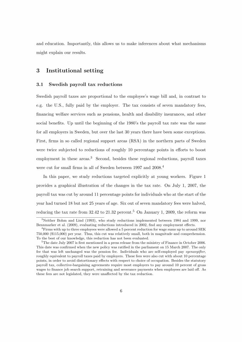
In this paper, we study reductions targeted explicitly at young workers. Figure 1

provides a graphical illustration of the changes in the tax rate. On July 1, 2007, the

payroll tax was cut by around 11 percentage points for individuals who at the start of the

year had turned 18 but not 25 years of age. Six out of seven mandatory fees were halved,

reducing the tax rate from 32.42 to 21.32 percent.5 On January 1, 2009, the reform was

3Neither Bohm and Lind (1993), who study reductions implemented between 1984 and 1999, norBennmarker et al. (2009), evaluating reductions introduced in 2002, find any employment effects.

4Firms with up to three employees were allowed a 5 percent reduction for wage sums up to around SEK750,000 ($115,000) per year. Thus, this cut was relatively small, both in magnitude and comprehension.To the best of our knowledge, this reduction has not been evaluated.

5The date July 2007 is first mentioned in a press release from the ministry of Finance in October 2006.This date was confirmed when the new policy was ratified in the parliament on 15 March 2007. The onlyfee that was left unchanged was the pension fee. Individuals who are self-employed pay egenavgifter,roughly equivalent to payroll taxes paid by employers. These fees were also cut with about 10 percentagepoints, in order to avoid distortionary effects with respect to choice of occupation. Besides the statutorypayroll tax, collective-bargaining agreements require most employers to pay around 10 percent of grosswages to finance job search support, retraining and severance payments when employees are laid off. Asthese fees are not legislated, they were unaffected by the tax reduction.

6

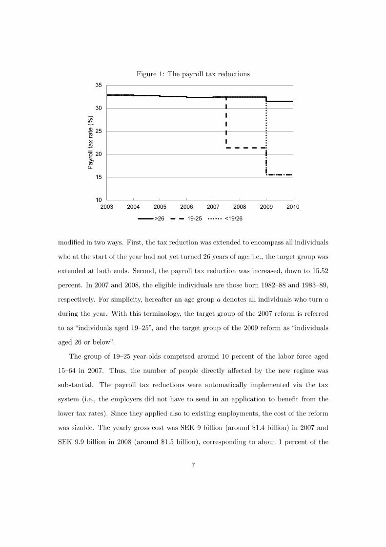
Figure 1: The payroll tax reductions

10

15

20

25

30

35

2003 2004 2005 2006 2007 2008 2009 2010

Payr

oll t

ax ra

te (%

)

>26 19-25 <19/26

modified in two ways. First, the tax reduction was extended to encompass all individuals

who at the start of the year had not yet turned 26 years of age; i.e., the target group was

extended at both ends. Second, the payroll tax reduction was increased, down to 15.52

percent. In 2007 and 2008, the eligible individuals are those born 1982–88 and 1983–89,

respectively. For simplicity, hereafter an age group a denotes all individuals who turn a

during the year. With this terminology, the target group of the 2007 reform is referred

to as “individuals aged 19–25”, and the target group of the 2009 reform as “individuals

aged 26 or below”.

The group of 19–25 year-olds comprised around 10 percent of the labor force aged

15–64 in 2007. Thus, the number of people directly affected by the new regime was

substantial. The payroll tax reductions were automatically implemented via the tax

system (i.e., the employers did not have to send in an application to benefit from the

lower tax rates). Since they applied also to existing employments, the cost of the reform

was sizable. The yearly gross cost was SEK 9 billion (around $1.4 billion) in 2007 and

SEK 9.9 billion in 2008 (around $1.5 billion), corresponding to about 1 percent of the

7

fiscal budget in these years. This figure increased substantially when the reductions were

extended, resulting in gross costs at SEK 17 billion ($2.6 billion) in 2009 and SEK 18

billion ($2.8 billion) in 2010.

3.2 Other relevant labor market reforms

With the purpose of increasing employment, both in general and for specific groups,

several labor market reforms were introduced in Sweden during 2007. First, temporary

subsidies for firms that hire individuals who have been unemployed or have received

sickness or disability benefits, New Start Jobs (NSJ), were introduced on January 1,

2007. In 2007–08, individuals aged 20–24 could apply for the subsidy after six months of

non-employment, whereas those who had turned 25 could apply only after twelve months

of non-employment—thus, in contrast to the payroll tax cut, it was the exact age that

mattered. In 2009, this cutoff was modified so that those who at the start of the year

have turned 20 but not 26 were eligible after six months.6 Consequently, in 2007–08 the

target groups overlapped, and from 2009 onwards they completely coincide. In principle,

this raises a concern that the employment estimates of the payroll tax reduction will be

contaminated. It turns out, however, that the number of applications for NSJ (available

in our data) was comparatively low, at about 0.5 percent of the ages 19–26, and the

difference in shares between the target group as a whole and 26-year-olds—the potential

bias of our estimates—is around 0.1 percentage points. We can thus conclude that this

is not a source of concern.

Second, income tax deductions were introduced in Sweden on January 1, 2007, with

the purpose of increasing labor supply in general. These deductions apply to all workers,

regardless of age, but we cannot rule out that there is heterogeneity in labor supply effects

with respect to age. If younger workers’ labor supply responded differently, we risk

6When introduced, the subsidy was equal in size to the payroll tax amount. In 2009, the size of thesubsidy increased to twice the payroll tax. The subsidy is given for a period equally long as the earliernon-employment spell and up to 5 years.

8

misestimating the effect of the payroll tax reductions. Edmark et al. (2012) show that

it is difficult to evaluate this deduction scheme due to the lack of unaffected comparison

groups; hence, we do not know exactly how different age groups responded. In this paper

we assume that the response was similar for individuals close in age.

Finally, a third reform concerns employment protection legislation. Loosening of

regulation in 2007 made it easier for employers to use fixed-term contracts. As temporary

work is relatively more widespread among young workers, employment (and wages) may

have been affected more for younger workers. However, Skedinger (2012) reports that

only 1.4 percent of all temporary workers were employed with the new regulations in

2008. The reform, thus, had little impact in practice.

3.3 Wage formation in Sweden

Wage setting in Sweden has traditionally been characterized by a high degree of central

bargaining. Over the last 10–15 years, there has been a substantial move toward the

decentralization of negotiations, but many workers still have centrally agreed wages and

this is likely to be more common for young workers.7 In 2007, between April and July,

central agreements covering 75 percent of all workers were renegotiated—i.e., before the

implementation of the 2007 reform but after its passing in the parliament in March 2007

(National Mediation Office 2007). New agreements were not made until 2010, one year

after the implementation of the new extended reductions.

Another institutional feature specific to the Swedish labor market is the fact that min-

imum wages are negotiated, not legislated as in most other OECD countries. Collective-

bargaining agreements differentiate wages based mainly on age, experience and levels

of skill. This means that younger workers are more likely to have wages bound by the

7Union density was at 80 percent in 1990 and 79 percent in 2000, and the share of workers coveredby collective-bargaining agreements is even higher. The influence given to the local bargaining partiesvaries by sector. The private sector, to which most young workers in Sweden belong, has a higher degreeof central wage setting than the public sector. See Fredriksson and Topel (2010) for a detailed discussionof the Swedish labor market.

9

minimum wage level.

4 Data

The data are collected by Statistics Sweden (SCB) and contain yearly information on

employment and demographical characteristics for all individuals living in Sweden at or

above 16 years of age in 2001–10 (the Louise and Rams data sets). The employment

data contain, for each individual and year, start and end months as well as total taxable

income from each employment source during the year. From this information we can de-

duce, for each individual and month, total monthly income from paid work. In addition,

we have access to detailed information on employment characteristics for a subsample of

all employees (measured between August and November each year), containing data on

actual monthly wages, work rate, industry affiliation of workplace, etc. For public sector

employers, the total population is surveyed through official registers, while firms in the

private sector are sampled using a stratification scheme.8 This subsample, in addition

to being used in the wage analysis, is also combined with the income data from the tax

registers to create monthly measures of employment for all individuals.

Our employment measure is constructed in the following way. Starting out from the

reduced sample of employed workers, for all individuals working at least 25 percent of

full-time, we partition the sample in cells defined by all unique combinations of age,

gender, three groups of education, firm sector (local/central public, blue-collar/white-

collar private), and year. For each cell, we calculate the 10th percentile of actual, full-

time equivalent wage; these values are to be used as cutoff values, serving as an income

criterion for full-time employment. These monthly cutoff values are matched to the tax

register data on all individuals. For each month that an individual’s taxable income

exceeds the appropriate cutoff value, she is, thus, classified as being full-time employed.

8The stratification is based on six firm size classes and 54 industry groups, giving a total of 324 strata.Stratification weights are included with the data and used in all wage analyses.

10

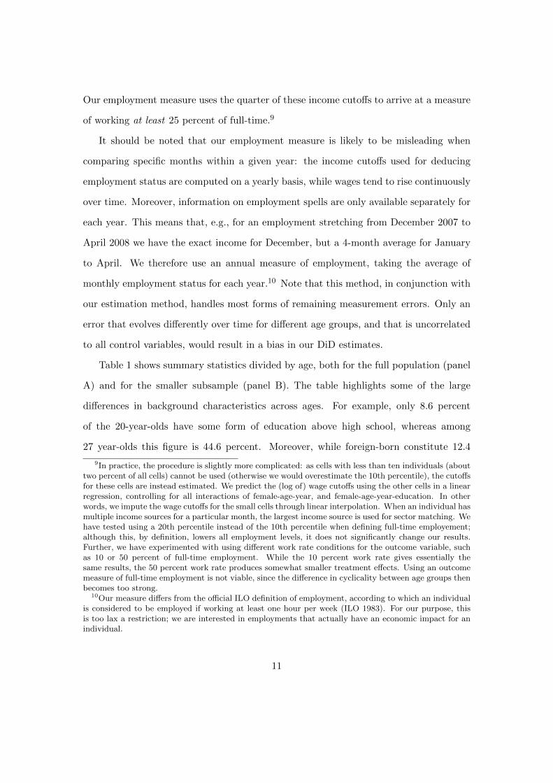
Our employment measure uses the quarter of these income cutoffs to arrive at a measure

of working at least 25 percent of full-time.9

It should be noted that our employment measure is likely to be misleading when

comparing specific months within a given year: the income cutoffs used for deducing

employment status are computed on a yearly basis, while wages tend to rise continuously

over time. Moreover, information on employment spells are only available separately for

each year. This means that, e.g., for an employment stretching from December 2007 to

April 2008 we have the exact income for December, but a 4-month average for January

to April. We therefore use an annual measure of employment, taking the average of

monthly employment status for each year.10 Note that this method, in conjunction with

our estimation method, handles most forms of remaining measurement errors. Only an

error that evolves differently over time for different age groups, and that is uncorrelated

to all control variables, would result in a bias in our DiD estimates.

Table 1 shows summary statistics divided by age, both for the full population (panel

A) and for the smaller subsample (panel B). The table highlights some of the large

differences in background characteristics across ages. For example, only 8.6 percent

of the 20-year-olds have some form of education above high school, whereas among

27 year-olds this figure is 44.6 percent. Moreover, while foreign-born constitute 12.4

9In practice, the procedure is slightly more complicated: as cells with less than ten individuals (abouttwo percent of all cells) cannot be used (otherwise we would overestimate the 10th percentile), the cutoffsfor these cells are instead estimated. We predict the (log of) wage cutoffs using the other cells in a linearregression, controlling for all interactions of female-age-year, and female-age-year-education. In otherwords, we impute the wage cutoffs for the small cells through linear interpolation. When an individual hasmultiple income sources for a particular month, the largest income source is used for sector matching. Wehave tested using a 20th percentile instead of the 10th percentile when defining full-time employement;although this, by definition, lowers all employment levels, it does not significantly change our results.Further, we have experimented with using different work rate conditions for the outcome variable, suchas 10 or 50 percent of full-time employment. While the 10 percent work rate gives essentially thesame results, the 50 percent work rate produces somewhat smaller treatment effects. Using an outcomemeasure of full-time employment is not viable, since the difference in cyclicality between age groups thenbecomes too strong.

10Our measure differs from the official ILO definition of employment, according to which an individualis considered to be employed if working at least one hour per week (ILO 1983). For our purpose, thisis too lax a restriction; we are interested in employments that actually have an economic impact for anindividual.

11

percent of the 20-year-olds, the same figure for 27-year-olds is 18.3 percent. These

differences are unlikely to be stable over time since they depend on, e.g, the state of the

economy, demographical changes and fluctuations in immigration. Panel B characterizes

the subsample of employed individuals, conditional on working at least a quarter of full-

time. As expected, both (full-time equivalent) montly wage and the work rate tend to

increase in age. Older workers are also increasingly tenured, public-sector employed,

higher educated and foreign-born. By comparing the two panels, we can deduce that,

e.g., those with low education, women and foreign-born have lower employment than

other groups.

Finally, we take a look at the evolution of employment and wages over time. Figure 2

gives the age distribution of employment before and after the 2007 payroll tax reduction.

There are two things to notice in the figure. First, there is a relative employment increase

for 19–25 year olds in 2008. Second, within the target group, workers at age 21–24 seem to

have gained the most. This suggests that there exists an employment effect, and that the

effect is decreasing in age. However, we know that, in general, younger workers perform

better in economic expansions, so the relative increase in employment may simply be a

result of the growing Swedish economy in 2006–08. This problem is further discussed in

the next section. In figure 3, we depict the corresponding distributional change in wages.

As seen, there is no clear-cut evidence of larger wage growth for younger workers.

5 Identification

5.1 Modelling the counterfactual outcome

We use two different estimation techniques in parallel, both relying on the Difference-

in-Differences (DiD) framework.11 In its simplest form, DiD uses the evolution of the

11While using a regression discontinuity design on the 25–26 age threshold might, prima facie, appearattractive, it is clear from figure 2 that such a strategy is not viable. There are systematic discontinuitiesat each cohort boundary in 2006, before the tax reduction was implemented. This pattern has its maincause in the fact that it is year of birth that determines when a child starts school in Sweden (see

12

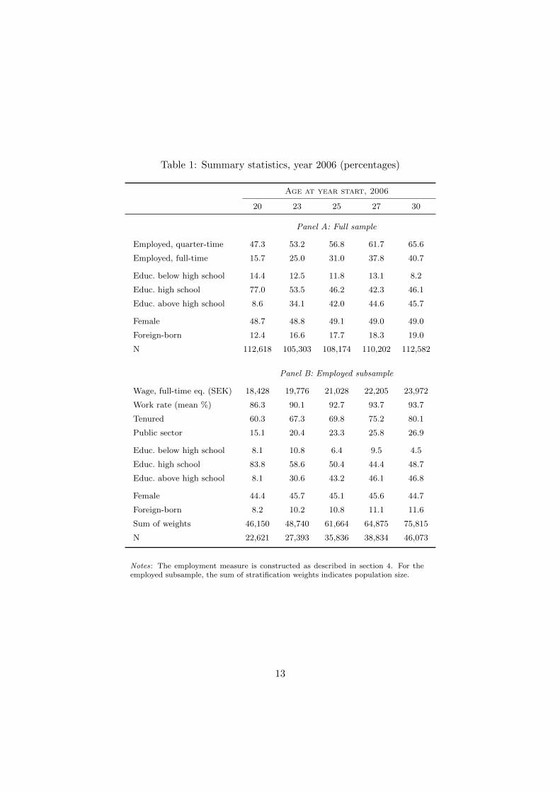
Table 1: Summary statistics, year 2006 (percentages)

Age at year start, 2006

20 23 25 27 30

Panel A: Full sample

Employed, quarter-time 47.3 53.2 56.8 61.7 65.6

Employed, full-time 15.7 25.0 31.0 37.8 40.7

Educ. below high school 14.4 12.5 11.8 13.1 8.2

Educ. high school 77.0 53.5 46.2 42.3 46.1

Educ. above high school 8.6 34.1 42.0 44.6 45.7

Female 48.7 48.8 49.1 49.0 49.0

Foreign-born 12.4 16.6 17.7 18.3 19.0

N 112,618 105,303 108,174 110,202 112,582

Panel B: Employed subsample

Wage, full-time eq. (SEK) 18,428 19,776 21,028 22,205 23,972

Work rate (mean %) 86.3 90.1 92.7 93.7 93.7

Tenured 60.3 67.3 69.8 75.2 80.1

Public sector 15.1 20.4 23.3 25.8 26.9

Educ. below high school 8.1 10.8 6.4 9.5 4.5

Educ. high school 83.8 58.6 50.4 44.4 48.7

Educ. above high school 8.1 30.6 43.2 46.1 46.8

Female 44.4 45.7 45.1 45.6 44.7

Foreign-born 8.2 10.2 10.8 11.1 11.6

Sum of weights 46,150 48,740 61,664 64,875 75,815

N 22,621 27,393 35,836 38,834 46,073

Notes: The employment measure is constructed as described in section 4. For theemployed subsample, the sum of stratification weights indicates population size.

13

Figure 2: Employment rates by age, 2006 and 2008

45

50

55

60

65E

mp

loym

en

t, y

ea

rly a

ve

rag

e (

%)

20 21 22 23 24 25 26 27 28

2006 2008

Notes: Employment is defined as working at least quarter−time. The vertical line indicates the age cutoff for the 2007 reform.

Figure 3: Average wage by age, 2006 and 2008 (log scale)

18000

20000

22000

24000

26000

28000

Mo

nth

ly w

ag

e (

in S

EK

)

19 20 21 22 23 24 25 26 27 28 29 30 31 32 33 34 35

2006 2008

Notes: Sample conditional on working at least quarter−time. For those working less than full−time, wage is scaled to its full−time equivalent. The vertical line indicates the age cutoff for the 2007 reform.

14

control group over time as a measure of how the treatment group would have evolved,

had the intervention not taken place. This results in the identifying assumption

E[y0i,t | Tr = 1

]= E

[y0i,t | Tr = 0

]+ α, (1)

where y0i,t is the no-treatment outcome for individual i at time t. In other words, the

counterfactual outcome of the treatment group is identical to the actual outcome of the

control group, except for a constant α. Figure 4 below demonstrates that, in the present

context, this is too strong an assumption. Inspecting the evolution of employment in

the period before the reform (2001–06), it is clear that individuals of different ages differ

in the degree of employment cyclicality, with younger workers tending to display larger

cyclical variations.12 As 2007 coincided with an economic expansion, comparing, say,

20-year-olds to 26-year-olds would result in an upward-biased reform estimate: even in

absence of a reform, a relative employment increase for 20-year-olds would have been

expected solely due to this group’s higher employment cyclicality. In addition to this

systematic age heterogeneity, there are idiosyncratic differences between cohorts (e.g.,

due to temporary waves of immigration).

In order to model the counterfactual outcome of the treatment group we use two

different approaches in tandem. The first method consists of supplementing the basic

DiD model with a large number of covariates. The estimated specification is

yi,t = δt ·D(i, t) + x′i,tβ + εi,t, (2)

where yi,t ∈ [0, 1] is average employment status in year t, D(i, t) is a treatment indicator

for individual i in year t, δt is the DiD estimate for year t, and xi,t is a vector of control

Fredriksson and Ockert 2005). With a DiD design, we assume that these cohort discontinuities areconstant over time, for each age pair.

12This heterogeneity is caused by, among other things, differences in labor market attachment, educa-tional attainment and social situation. See Hoynes et al. (2012) for an extensive treatment of employmentcyclicality for the U.S. labor market.

15

Figure 4: Employment trends for different age groups

40

50

60

70E

mp

loym

en

t, y

ea

rly a

ve

rag

e (

%)

2001 2002 2003 2004 2005 2006 2007 2008 2009 2010

20 25 26

27 30

Notes: Employment is defined as working at least quarter−time. The two vertical lines indicate the reform years.

variables, capturing a multitude of factors that may influence the probability of being

employed. These include dummy variables for year, age, county of birth (including

indicator for foreign-born), gender, geography, and whether the parents immigrated

into Sweden. For foreign-borns, we also control for country of birth and years since

immigration into Sweden.

The previous technique models the covariates in equation (2) in a linear functional

form. That is, we require the identifying assumption

E[y0i,t | X = xi,t

]= x′

i,tβ (3)

to hold for individuals of both the treatment and control groups. However, there are

likely to be structural differences between the metropolitan and the rural parts of Sweden

due to, e.g., differences in industrial structure and demographics. Since, additionally,

the size and composition of cohorts vary over time across Sweden (e.g., through immi-

16

gration), linear controls may be inadequate. For this reason, we also use DiD with an

exact-matching approach. Specifically, treatment-control group pairs are matched with

respect to local labor markets, and for each matched pair the (standard) DiD estimator

is used to obtain the average treatment effect of the treated (ATT).13 The identifying

assumption required is similar to assumption (3), except that we now condition on local

labor markets, L:

E[y0i,t | X = xi,t, L = l

]= x′

i,tβl (4)

The overall ATT is obtained by averaging the ATTl:s for all subgroups L = l,

weighted by the distribution of L in the treatment group. Formally, for each time

period, t,

ATTt =∑l∈L

ATTl,t ·# {i : Tr = 1, T = t, L = l}

# {i : Tr = 1, T = t}

where ATTl is the DiD estimate for the local labor market l. Most of our covariates

that are intended to control for important compositional variations over time capture

labor-market specific circumstances, such as integration of immigrants in the labor mar-

ket. The rationale for matching on local labor markets is that the dynamics of these

circumstances may differ across Sweden. Since local labor markets cover entire commut-

ing areas, they should be less sensitive to endogeneity concerns than had we used a finer

regional division.14

To summarize, the difference between our two methods lie in how the counterfactual

outcome of the treatment group is modelled, as formalized by equations (3) and (4).

13The concept of local labor market is conceived of by Statistics Sweden. Based on workers’ commutingpatterns, Sweden is divided into 75 broad commuting areas. Thus, commuting mostly takes place within,but not between, separate local labor markets. We have also experimented with matching on whetherforeignborn, and on gender, but this gives very similar results. Evidently, our linear controls are sufficientfor these dimensions.

14Blundell et al. (2004) use propensity score matching to evaluate the employment effects of a manda-tory job search program in the U.K. The fact that we match on a single, discrete variable, in combinationwith a large number of observations, allows us to use exact matching. Compared to propensity scorematching, exact matching is less dependent on functional assumptions.

17

By approaching the identification problem from two slightly different angles we should

obtain a more robust overall picture. In particular, if the two methods produce similar

estimates, we consider the results credible.

5.2 Absolute versus relative effects

An implication of the DiD identifying assumption of parallel trends is that the control

group must not be affected by the intervention. If such treatment spillovers exist, we will

not measure the difference between the reform outcome and the counterfactual outcome,

but the difference to the control group deviation from its counterfactual outcome. In

other words, we obtain a measure of the relative rather than the absolute effect of the

reform. In the present case, there are strong reasons to suspect that the tax reduction

had an indirect impact also on individuals not in the target group. The treatment

spillover takes the form of substitution and scale effects. As a way of illustration, consider

individuals at 25–26 years of age. The 2007 payroll tax reduction increases the cost of

26-year-old labor relative to 25-year-old labor. If firms consider 25-year-olds and 26-

year-olds as substitute inputs they will, all else equal (i.e. holding output constant),

lower demand for the latter group of workers, resulting in a negative substitution effect

for 26-year-old labor. The magnitude of the negative substitution effect on non-treated

individuals should depend on their similarity to individuals in the target group. Hence,

the effect should decrease in age.

The scale effect tends to work in the opposite direction to the substitution effect. A

factor input price drop results in a downward shift of the firms’ cost functions, potentially

causing them to expand output. Similar to income effects in consumer theory, the sign of

the scale effect can be either positive or negative, but for normal factor inputs, demand

is increasing in output. If employers prefer older, more experienced, workers, the scale

effect increases in age. Nonetheless, this scale effect asymmetry, if it exists, is likely to

be small, especially if we use treatment-control pairs that are close in age. Hence, the

18

substitution effect bias is, arguably, the bigger problem.

5.3 Choice of comparison groups

The previous discussion suggests that there is an element of trade-off involved when

choosing comparison groups: decreasing the age interval around the cutoff should get us

closer to estimating a causal, albeit relative, treatment effect, but the estimate is unlikely

to be generalizable to the target group as a whole. With this in mind, we evaluate the

effects of the payroll tax reduction both for 25-year-olds, and for the whole target group,

19–25 year-olds.

The parallel trends assumption is, by definition, not testable since it concerns coun-

terfactual outcomes. A common convention is to consider the evolution of the treatment

and control groups prior to the intervention, thus getting an indication on whether the

assumption is likely to hold. (Or rather, when it is not likely to hold.) While this pro-

cedure does not guarantee unbiased estimates, as is clear from the above discussion of

treatment spillover effects, we consider parallel pre-treatment trends a minimal condition.

This constrains us to use control group individuals close to the treatment cutoff, mainly

26-year-olds. As discussed above, these individuals are probably negatively affected by

the reform and, thus, we interpret the estimations as upper bounds of the employment

effect for the target group. As a special case, we consider individuals within a small

bandwidth just around the treatment cutoff, comparing 25-year-olds born in January–

March with 26-year-olds born in October–December. This specification has elements of

a regression discontinuity design, but with controlling for the pre-reform discontinuity.

While heterogeneous cyclicality should no longer be an issue, with comparison group so

close in age, this comes at a cost: similar to RD designs in general, the estimates risk

being only locally valid.

In theory, we should expect stronger treatment effects for younger workers since the

remaining available treatment years (treatment dose) is decreasing in age. Estimating

19

effects for individuals close to the cutoff may, for this reason, underestimate the average

treatment effect on the treated. Additionally, since the treatment and control groups are

defined in terms of age groups they are each year redefined in terms of cohorts. Conse-

quently, an estimate based on single age groups is more sensitive to cohort heterogeneity,

showing up as year shocks. In contrast, when using a treatment group of multiple ages,

this heterogeneity is averaged out.15 Another way of dealing with this issue is to es-

timate pooled treatment effects for two years at a time, e.g., the 2007–08 effect. Such

an approach averages out cohort offsets, but at a loss in temporal resolution. We have

chosen to use the more transparent yearly estimates when presenting the main results.

In the cost-benefit analysis, however, we utilize the pooled estimates in order to get more

robust measures. (When cohorts are roughly of the same size, the joint estimate will be

close to the average of its corresponding yearly components.)

5.4 Repeated treatment and the 2009 extension

A difficulty with our method of evaluation is that, with time, it gets increasingly difficult

to find individuals who have not been previously subjected to the payroll tax reduction.

This makes it hard to identify the reform effect for the later years in our sample. Es-

sentially, the problem of lagged treatment exists whenever employment spells extend

from one year to the next. Figur 5 illustrates how different cohorts are subjected to the

payroll tax reductions. In 2007, the target group consists of individuals born 1982–88.

Their natural control group consists of individuals that are slightly older, i.e., those

born 1981. In 2008, individuals born 1983–89 are in the target group, and those born

1982 constitute the control group. Arguably, the employment estimate for 2007 is best

identified since there is no earlier intervention, for any age group. Already in 2008, the

15Insofar as this cohort heterogeneity consists of compositional differences in dimensions that we ob-serve, our control variables should take care of the problem. However, a constant offset for, say, thecohort of 25-year-olds in 2007 would bias the estimate of the reform effect. Cohort heterogeneity inthe control group remains a potential problem since we, in most cases, cannot extend the age-intervalupwards.

20

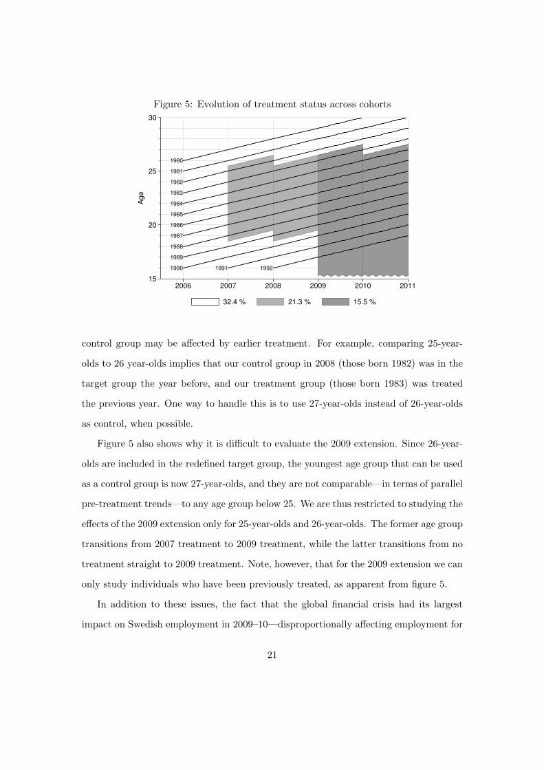
Figure 5: Evolution of treatment status across cohorts

1980

1981

1982

1983

1984

1985

1986

1987

1988

1989

1990 1991 1992

15

20

25

30

Age

2006 2007 2008 2009 2010 2011

32.4 % 21.3 % 15.5 %

control group may be affected by earlier treatment. For example, comparing 25-year-

olds to 26 year-olds implies that our control group in 2008 (those born 1982) was in the

target group the year before, and our treatment group (those born 1983) was treated

the previous year. One way to handle this is to use 27-year-olds instead of 26-year-olds

as control, when possible.

Figure 5 also shows why it is difficult to evaluate the 2009 extension. Since 26-year-

olds are included in the redefined target group, the youngest age group that can be used

as a control group is now 27-year-olds, and they are not comparable—in terms of parallel

pre-treatment trends—to any age group below 25. We are thus restricted to studying the

effects of the 2009 extension only for 25-year-olds and 26-year-olds. The former age group

transitions from 2007 treatment to 2009 treatment, while the latter transitions from no

treatment straight to 2009 treatment. Note, however, that for the 2009 extension we can

only study individuals who have been previously treated, as apparent from figure 5.

In addition to these issues, the fact that the global financial crisis had its largest

impact on Swedish employment in 2009–10—disproportionally affecting employment for

21

younger workers—makes identification for these years even more difficult. When con-

sidering the 25-year-olds, the 2009 estimate will measure the impact of an extended

reduction in the wake of the financial crisis. For 26-year-olds, we, correspondingly, get

the effect of introducing a payroll tax reduction in the wake of an economic depression.

Hence, both of these specifications could be seen as testing how the payroll tax reduction

fare when labor market conditions worsen.

5.5 Estimating wage effects

The impact on employment depends on how much of the tax cut is shifted onto workers

in the form of higher wages. In the long run, wages may adjust to counteract the effect of

a payroll tax change. In the extreme case of full shifting, the payroll tax decrease will be

fully cancelled out by wage increases, resulting in unchanged net labor costs for employers

and, consequently, no employment effects. In the present case, with targeted reductions

and a target group that has little attachment to the labor market, it is difficult, ex ante,

to predict whether shifting will occur.16

Wage effects can appear through two channels: individual bargaining and union

bargaining. In the latter case, there is a possibility that unions seek to make sure that

all workers benefit so that the payroll tax reductions resulted in general shifting. This

gives rise to a problem similar to when estimating employment effects: the δ in equation 2

captures only the relative wage effect. However, the primary question we are interested

in is not whether shifting occurred per se; rather, our focus is on whether relative wage

increases around the cutoff can explain (the lack of) relative changes in employment.

As young workers’ wages are predominantly centrally negotiated, there is less concern

for regional differences across Sweden and we, therefore, refrain from matching on local

labor markets (the matched DiD results are similar to those reported in the paper).

16Some guidance may be found in Kolm (1998), who considers a two-sector (general equilibrium) modelwhere market competitiveness differs between sectors, and where a general payroll tax cut would be fullyshifted to workers. In this model unemployment can be reduced by taxing the less competitive sectorrelatively more.

22

Finally, it is important to stress that we only study the immediate impact on wages. If

wage adjustments appear in the longer run, we will underestimate the long-term general

equilibrium consequences of the payroll tax cuts.

6 Results

6.1 Main findings

Table 2 presents the main results for the 2007 reduction. The outcome variable is yearly

average employment status, ranging from zero to one, and for each treatment-control pair

we report the estimates from both DiD methods side by side. All treatment effects are

relative to the reference period 2001–04. The first two rows show whether the comparison

groups move in parallel prior to the 2007 reform: significant pre-treatment effects for

2005 or 2006 would indicate that the control group is invalid.17

The first four columns study the effect at the treatment cutoff. Starting with the

smallest bandwidth, we compare the three oldest birthmonth cohorts (born in January–

March) of the 25-year-olds with the three youngest birthmonth cohorts (born in October–

December) of the 26-year-olds. Arguably, in these specifications the issue of heterogenous

cyclicality should be minor, implying that any relative difference that we observe is most

likely caused by the reform. The DiD with linear controls shows a statistically significant,

albeit small, positive employment effect, both in 2007 and in 2008. For the matched DiD,

point estimates are almost identical but precison is lower.18 From the local estimation

17Another method sometimes used in the literature is to run separate placebo regressions for selectedyears. Our method is, arguably, less arbitrary since we calculate pre-reform effects routinely for everyspecification used. Naturally, these estimates should be taken with a critical view: as the null hypothesisis that of parallel trends, violations of the identifying assumption may be too difficult to discover.Conversely, we are also likely to have some instances of false positives (specifically, in roughly oneregression out of twenty when using the conventional 5-percent significance level).

18A potential reason for the lack of significance is that bootstrapping overestimates standard errorswhen the number of observations are too small. But it is also possible that the OLS cluster-adjustedstandard errors are underestimated—note that the latter rely on stronger assumptions than the standarderrors obtained by bootstrapping. Be that as it may, the two methods conform (in terms of statisticalsignificance) as the sample size grows.

23

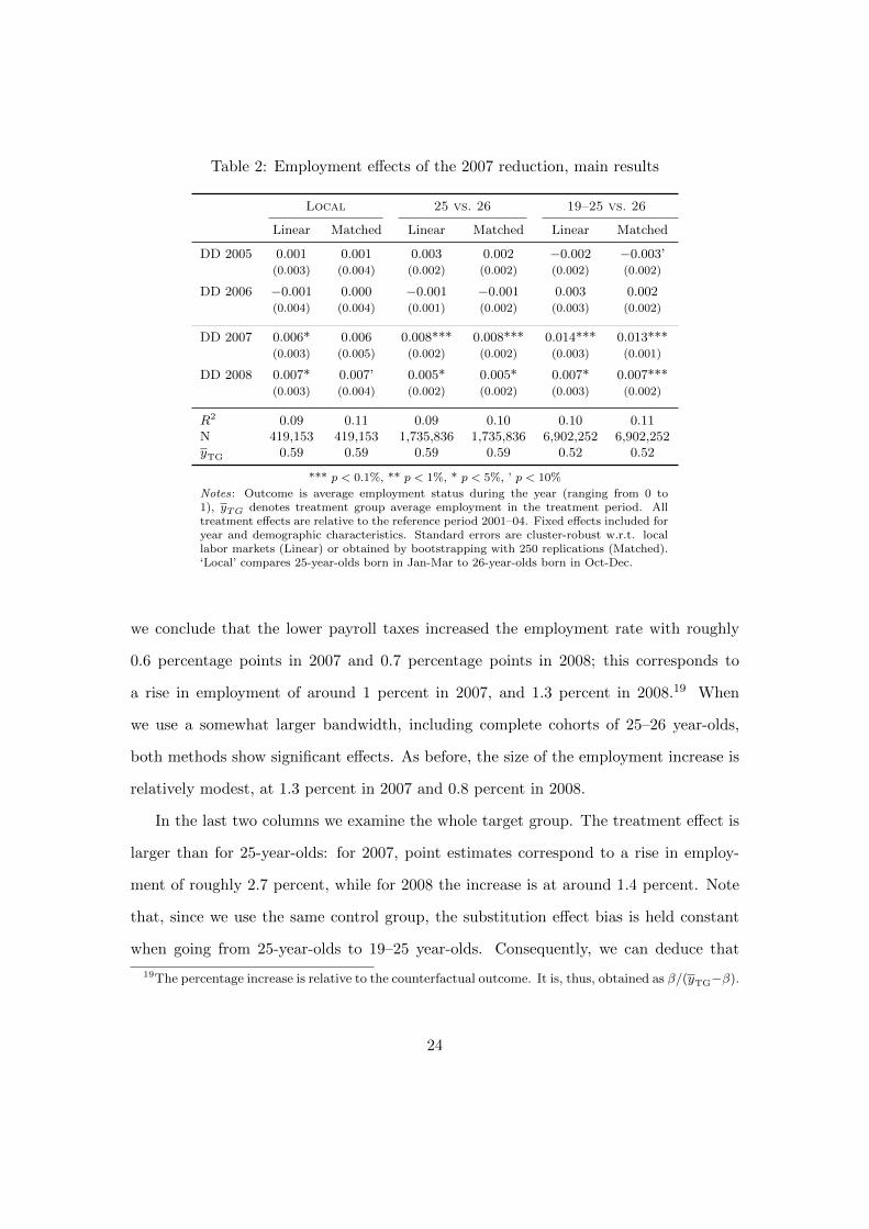
Table 2: Employment effects of the 2007 reduction, main results

Local 25 vs. 26 19–25 vs. 26

Linear Matched Linear Matched Linear Matched

DD 2005 0.001 0.001 0.003 0.002 −0.002 −0.003’(0.003) (0.004) (0.002) (0.002) (0.002) (0.002)

DD 2006 −0.001 0.000 −0.001 −0.001 0.003 0.002(0.004) (0.004) (0.001) (0.002) (0.003) (0.002)

DD 2007 0.006* 0.006 0.008*** 0.008*** 0.014*** 0.013***(0.003) (0.005) (0.002) (0.002) (0.003) (0.001)

DD 2008 0.007* 0.007’ 0.005* 0.005* 0.007* 0.007***(0.003) (0.004) (0.002) (0.002) (0.003) (0.002)

R2 0.09 0.11 0.09 0.10 0.10 0.11N 419,153 419,153 1,735,836 1,735,836 6,902,252 6,902,252yTG 0.59 0.59 0.59 0.59 0.52 0.52

*** p < 0.1%, ** p < 1%, * p < 5%, ’ p < 10%

Notes: Outcome is average employment status during the year (ranging from 0 to1), yTG denotes treatment group average employment in the treatment period. Alltreatment effects are relative to the reference period 2001–04. Fixed effects included foryear and demographic characteristics. Standard errors are cluster-robust w.r.t. locallabor markets (Linear) or obtained by bootstrapping with 250 replications (Matched).‘Local’ compares 25-year-olds born in Jan-Mar to 26-year-olds born in Oct-Dec.

we conclude that the lower payroll taxes increased the employment rate with roughly

0.6 percentage points in 2007 and 0.7 percentage points in 2008; this corresponds to

a rise in employment of around 1 percent in 2007, and 1.3 percent in 2008.19 When

we use a somewhat larger bandwidth, including complete cohorts of 25–26 year-olds,

both methods show significant effects. As before, the size of the employment increase is

relatively modest, at 1.3 percent in 2007 and 0.8 percent in 2008.

In the last two columns we examine the whole target group. The treatment effect is

larger than for 25-year-olds: for 2007, point estimates correspond to a rise in employ-

ment of roughly 2.7 percent, while for 2008 the increase is at around 1.4 percent. Note

that, since we use the same control group, the substitution effect bias is held constant

when going from 25-year-olds to 19–25 year-olds. Consequently, we can deduce that

19The percentage increase is relative to the counterfactual outcome. It is, thus, obtained as β/(yTG−β).

24

the increase in treatment effect represents an absolute increase. The larger effect for

younger individuals is consistent with treatment dose effects: younger individuals have

longer expected exposure to the reduced payroll tax. However, this difference may also

depend on labor force composition. For example, if low-skilled jobs are affected more by

lower payroll taxes and younger individuals to a larger extent are low-skilled, we would

expect the treatment effect to decrease in age.

Both for 25-year-olds and for the whole target group the treatment effect is smaller

in 2008 than in 2007. As discussed in section 5, if the treatment effect for one year

persists to the following year, using 26-year-olds as the control group will bias the 2008

estimate downwards. In table A.1 in the appendix, we address this issue by comparing

25-year-olds to 27-year-olds. While the 2007 estimate is essentially the same, the 2008

estimate is now much larger. In fact, when using 27-year-olds as the control group, the

effect increases over time. Since we know that the control group has not been previously

treated, this result is consistent with the possibility of a lagged treatment effect for the

treatment group. It is, however, important to stress that these results may, instead, be

due to cohort heterogeneity; changing the control group age is equivalent to changing the

control group cohort for each year. By pooling 26–27 year-olds in the control group, we

should to some extent net out cohort heterogeneity. Indeed, this gives almost identical

employment effects in 2007 and 2008, at roughly 1.3 percent. Unfortunately, in most of

our specifications we cannot include individuals older than 26 years old in the control

group. Thus, in what follows we use a control group of 26-year-olds. (As an example, the

last two columns of table A.1 show that pitting 19–25 year-olds against 26–27 year-olds

results in non-parallel pre-treatment trends, and so we cannot test whether the 2008

effect for 19–25 year-olds is downward biased as well.)

In 2009, the payroll tax was further reduced for young workers, the results of which

are presented in table 3. Columns 1–2 demonstrate that the extended reductions did

not further boost employment for 25-year-olds in 2009–10; the estimates seem to be

25

roughly similar to those of the initial 2007 reform. (As 26-year-olds are part of the target

group from 2009 and onwards, we have switched to using 27-year-olds as the frame of

reference.) In columns 3–4 we study 26-year-olds, who were subjected to reduced payroll

taxes for 2009 onwards, but not before. While there are significant estimates in 2008—

possibly due to a lagged treatment effect—there is no evidence of an employment effect

of the 2009 extension. However, as we discuss in section 5, there are two reasons for

why we should be cautious in interpreting these results: all examined individuals were

previously treated, and the 2009 extension coincided with a severe slump in the Swedish

economy, and so it is not possible to isolate the effect of the extension from asymmetrical

employment effects of the downturn (any symmetrical effect would be handled by the

methods applied). We can, however, establish that if the additional reduction had an

impact on 25 year-olds, this impact was not large enough to counteract the effects of the

economic downturn.

Because of treatment spillovers, the estimates presented above are likely to be upward-

biased measures of the absolute employment increase. However, since for any specific

year, the reported treatment effect estimate is the sum of the treatment effect for the

treatment group and the negative substitution effect for the control group, we can get an

idea of the magnitude of this bias by comparing different specifications. In particular,

we can use the 25–26 estimates in columns 3–4 of table 2 as an upper bound for the

negative substitution effect for the 26-year-olds, and hence, as an upper bound for the

substitution effect bias affecting estimations for the entire target group. Consequently,

the absolute employment increases for the age group 19–25 are at least around 0.6 and

0.2 percentage points in 2007 and 2008, respectively. Leaving control group substitution

aside, it is an open question whether the estimated employment increase in the target

group occurred at the cost of substitution with even older individuals in the labor mar-

ket. That is, even when taking the control group substitution bias into account, the

remaining employment effect is still likely to overestimate the net employment effect in

26

Table 3: Employment effects of the 2009 extension

25 vs. 27 26 vs. 27

Linear Matched Linear Matched

DD 2005 0.002 0.002 −0.001 −0.001(0.002) (0.002) (0.002) (0.002)

DD 2006 0.001 0.001 0.003 0.003(0.002) (0.002) (0.002) (0.002)

DD 2007 0.007*** 0.007*** −0.001 −0.001(0.002) (0.002) (0.002) (0.002)

DD 2008 0.010*** 0.010*** 0.005*** 0.005**(0.002) (0.002) (0.002) (0.002)

DD 2009 0.005*** 0.005* 0.001 0.000(0.001) (0.002) (0.001) (0.002)

DD 2010 0.009*** 0.009*** 0.002 0.002(0.002) (0.002) (0.002) (0.002)

R2 0.10 0.11 0.11 0.11N 2,214,808 2,214,808 2,224,418 2,224,418yTG 0.57 0.57 0.59 0.59

*** p < 0.1%, ** p < 1%, * p < 5%, ’ p < 10%

Notes: See notes for table 2.

the economy. This issue is further discussed in section 8.

In summary, there seem to have been positive, but small, employment effects of the

2007 payroll tax reduction. This holds irrespective of whether we study a small interval

around the treatment cutoff, or examine the whole target group of 19–25 year-olds. For

the 2009 extended reduction, there is no evidence of any additional effect.

6.2 Treatment effect heterogeneity

We next turn to the subsample of young immigrants, in table 4. This group, which

constituted about 15 percent of the age group 19–25 in 2007–08, is characterized by

weak attachment to the Swedish labor market. The employment rate for this group is

20 percentage points lower than for the whole population of young workers, as reported

in the bottom rows of tables 2 and 4. Strikingly, there is no evidence that the payroll tax

27

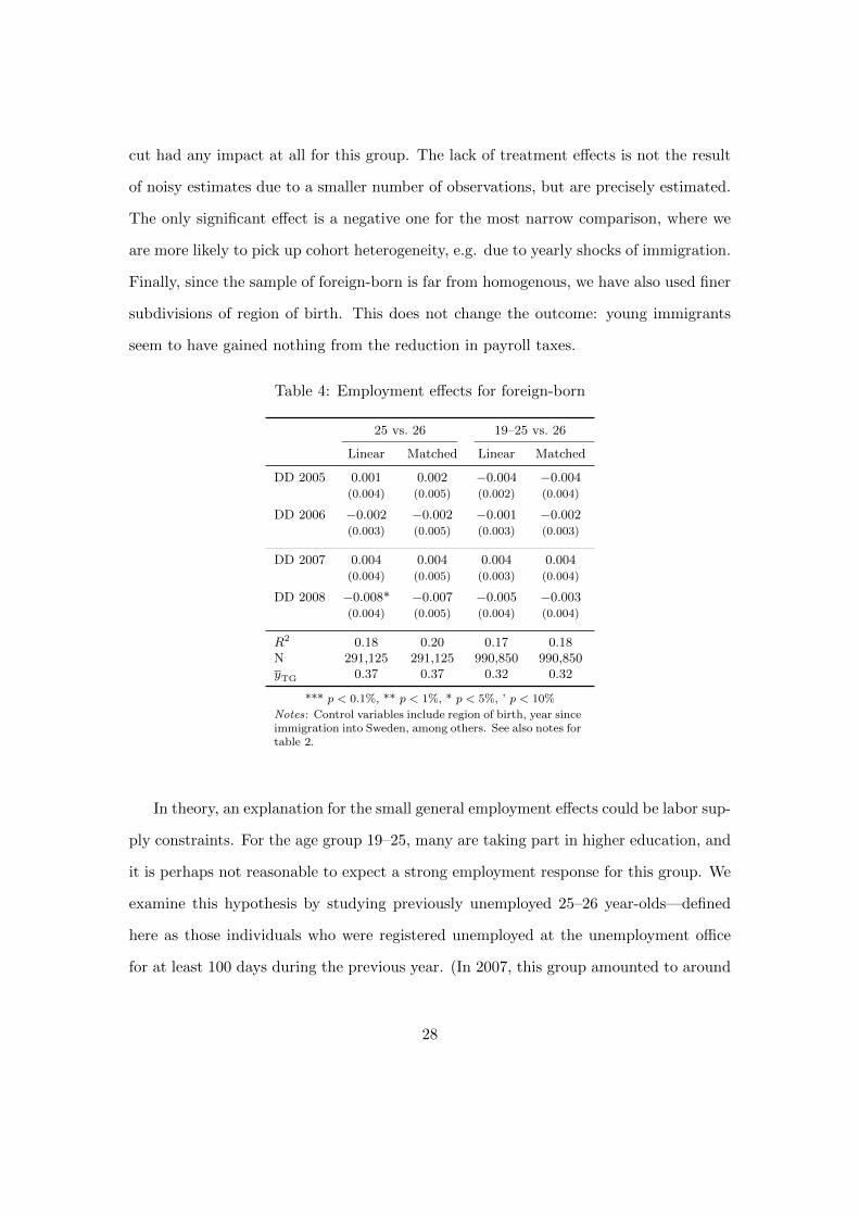
cut had any impact at all for this group. The lack of treatment effects is not the result

of noisy estimates due to a smaller number of observations, but are precisely estimated.

The only significant effect is a negative one for the most narrow comparison, where we

are more likely to pick up cohort heterogeneity, e.g. due to yearly shocks of immigration.

Finally, since the sample of foreign-born is far from homogenous, we have also used finer

subdivisions of region of birth. This does not change the outcome: young immigrants

seem to have gained nothing from the reduction in payroll taxes.

Table 4: Employment effects for foreign-born

25 vs. 26 19–25 vs. 26

Linear Matched Linear Matched

DD 2005 0.001 0.002 −0.004 −0.004(0.004) (0.005) (0.002) (0.004)

DD 2006 −0.002 −0.002 −0.001 −0.002(0.003) (0.005) (0.003) (0.003)

DD 2007 0.004 0.004 0.004 0.004(0.004) (0.005) (0.003) (0.004)

DD 2008 −0.008* −0.007 −0.005 −0.003(0.004) (0.005) (0.004) (0.004)

R2 0.18 0.20 0.17 0.18N 291,125 291,125 990,850 990,850yTG 0.37 0.37 0.32 0.32

*** p < 0.1%, ** p < 1%, * p < 5%, ’ p < 10%

Notes: Control variables include region of birth, year sinceimmigration into Sweden, among others. See also notes fortable 2.

In theory, an explanation for the small general employment effects could be labor sup-

ply constraints. For the age group 19–25, many are taking part in higher education, and

it is perhaps not reasonable to expect a strong employment response for this group. We

examine this hypothesis by studying previously unemployed 25–26 year-olds—defined

here as those individuals who were registered unemployed at the unemployment office

for at least 100 days during the previous year. (In 2007, this group amounted to around

28

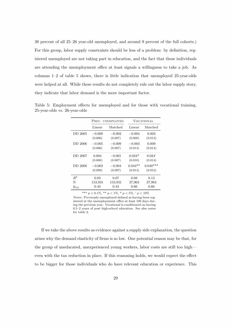
38 percent of all 25–26 year-old unemployed, and around 9 percent of the full cohorts.)

For this group, labor supply constraints should be less of a problem: by definition, reg-

istered unemployed are not taking part in education, and the fact that these individuals

are attending the unemployment office at least signals a willingness to take a job. As

columns 1–2 of table 5 shows, there is little indication that unemployed 25-year-olds

were helped at all. While these results do not completely rule out the labor supply story,

they indicate that labor demand is the more important factor.

Table 5: Employment effects for unemployed and for those with vocational training,25-year-olds vs. 26-year-olds

Prev. unemployed Vocational

Linear Matched Linear Matched

DD 2005 −0.000 −0.002 −0.004 0.003(0.006) (0.007) (0.009) (0.013)

DD 2006 −0.005 −0.009 −0.003 0.009(0.006) (0.007) (0.014) (0.014)

DD 2007 0.004 −0.001 0.024* 0.024’(0.008) (0.007) (0.010) (0.014)

DD 2008 −0.003 −0.004 0.044** 0.048***(0.009) (0.007) (0.014) (0.012)

R2 0.03 0.07 0.08 0.13N 153,931 153,931 37,963 37,963yTG 0.43 0.43 0.66 0.66

*** p < 0.1%, ** p < 1%, * p < 5%, ’ p < 10%

Notes: Previously unemployed defined as having been reg-istered at the unemployement office at least 100 days dur-ing the previous year. Vocational is conditioned on having0.5–2 years of post high-school education. See also notesfor table 2.

If we take the above results as evidence against a supply side explanation, the question

arises why the demand elasticity of firms is so low. One potential reason may be that, for

the group of uneducated, unexperienced young workers, labor costs are still too high—

even with the tax reduction in place. If this reasoning holds, we would expect the effect

to be bigger for those individuals who do have relevant education or experience. This

29

hypothesis is tested in columns 3–4 of table 5. Considering 25–26 year-olds with up to two

years of post high school vocational training, the employment response is considerably

larger than for the same age groups without conditioning: the relative increase is now

at around 3.8 percent in 2007 and 7 percent in 2008. While we do expect a stronger

employment response for this small subgroup, it is likely that there is also a high degree

of substitution bias at play: workers at age 25 and 26, additionally restricted to a well-

defined education level, should be close to perfect substitutes. In such an environment,

even a small difference in labor cost could result in large substitution effects

We conclude that the small employment response of the payroll tax cut does not

seem to be explained by lack of labor supply. It appears more likely that, in general,

labor costs for young workers are still too high in relation to expected productivity.

6.3 Wage effects

We next examine whether part of the payroll tax cut was passed on to employees as

higher wages. The outcome measure is now the log of monthly, full-time equivalent,

wage for those employed at least quarter-time (in symmetry with our main employment

definition used above). Table 6 gives the impacts of both the 2007 initial cut and the

2009 extension. Starting with the 2007 reduction, there is no effect around the cut-off;

the point estimates for 25-year-olds are small in economic terms, and insignificant. For

the target group as a whole there is, however, a small relative wage increase, slightly

above one percent both in 2007 and in 2008. This could indicate that some of the younger

workers of the target group have taken home a small fraction of the tax cut given to

employers. Notably, the wage increase for 19–25 year-olds shows up already in 2007.20

Next, we compare 25-year-olds not to 26-year-olds, but to 27-year-olds, studying the

evolution of wages into the 2009 extension. With this control group, we do find wage

20For each of the two age groups that we consider, we have tested for heterogeneity with respect toprivate or public sector, for blue collar or white collar workers, and for new or tenured employees. Theresults for these subgroups are similar to the general case.

30

Table 6: Wage effects of the 2007 reduction and the 2009 extension

2007 Reform 2009 Reform

25 vs. 26 19–25 vs. 26 25 vs. 27 26 vs. 27

DD 2005 −0.006 0.005’ −0.001 0.005(0.004) (0.003) (0.006) (0.004)

DD 2006 −0.005 0.006 −0.006* −0.001(0.004) (0.004) (0.003) (0.004)

DD 2007 0.004 0.012*** 0.007 0.003(0.003) (0.003) (0.004) (0.004)

DD 2008 0.004 0.013* 0.010** 0.006(0.005) (0.005) (0.003) (0.004)

DD 2009 0.007* 0.011**(0.003) (0.004)

DD 2010 0.007’ 0.004(0.004) (0.003)

R2 0.21 0.27 0.27 0.27N 537,619 1,615,138 701,024 739,208yTG 21,672.71 20,286.88 22,282.25 22,879.42

*** p < 0.1%, ** p < 1%, * p < 5%, ’ p < 10%

Notes: Outcome is the log of monthly full-time equivalent wage(truncated below to 0), yTG denotes treatment group average out-come in the treatment period, in non-log form. All treatment ef-fects are relative to the reference period 2001–04. Fixed effectsincluded for year and demographic characteristics. Standard er-rors are cluster-robust w.r.t. local labor markets.

effects in 2008, but also pre-treatment effects in 2006. As with employment, cohort

heterogeneity may be the reason for the difference compared to using a control group

of 26-year-olds. More importantly, there is no additional wage effect for 25-year-olds of

the 2009 extended reduction, nor do wages seem to adjust more in the longer run for

25-year-olds. Finally, in the last column, we examine the effect on relative wages of going

from no treatment to 2009 treatment, comparing 26-year-olds to 27-year-olds. The wage

effect for the 26-year-olds coincides with their switch of treatment status in 2009, but is

not apparent in 2010.

Understanding these wage effects requires making a few observations. To start with,

there are indications that the unions and the employer organizations agreed on letting

31

minimum wages increase faster than general wages after 2007 (National Mediation Office

2007). Thus, we are potentially picking up negotiated minimum wage increases. It is,

however, an open question whether these increases were the result of the reform or

part of a long-term trend. (As mentioned in section 3, wages were renegotiated at the

central level just after the passing of the 2007 reduction in the parliament. Hence,

since both the unions and the employer organizations were aware of the forthcoming

tax reduction there is, in principle, a possibility that the wage response came before the

actual implementation.) What speaks against the minimum wage increase explanation

is the evidence of wage effects even for age groups that typically have wages strictly

above the minimum wage level.21 Another potential explanation is that shifting works

through individual wage bargaining. Such an impact, if it exists, is likely to be more

immediate than union-negotiated wage increases. Having said this, we conclude that

given the small size of the wage increase, shifting cannot by itself explain the modest

employment effects we have found.

7 Cost-benfit analysis

In the following, we present some further metrics for evaluating the payroll tax reduc-

tion, with emphasis on 2007–08 where we have the most credible identification. When

calculating demand elasticity and cost per job, we choose to reestimate the models, using

pooled treatment effect estimates for 2007–08. Averaging effects over two years has the

effect of reducing cohort heterogeneity in the control group, thus producing more robust

estimates on which to base our derived measures. It is important to stress, however, that

these derived measures are likely to be overly optimistic. First, the substitution effect

bias causes us to overestimate the treatment effect and, consequently, to overestimate

the demand elasticity and underestimate the cost per job. Second, it is by no means

21Forslund et al. (2012) report that young workers’ wages in the private sector are often higher thanthe negotiated minimum wages, even for workers as young as 19 years old.

32

clear that the target group employment increase reflects a net increase of jobs in the

economy. Rather, a part of this increase may be at the expense of older workers in

the labor force. Although this will not affect the elasticity estimate—which is defined

as being with respect to young labor—it will further bias the measure of cost per job,

as job losses for older workers are not taken into account. This is discussed further in

section 8.

7.1 Elasticities

We can combine the employment and wage estimates to get estimates of the elasticity

of demand for young workers with respect to labor costs. For the target group as a

whole, the 2007–08 employment increase is 2 percent, and the 2007–08 wage increase

is 1.2 percent. Hence, we arrive at a labor demand elasticity at about −0.31. The

corresponding figure for 25-year-olds is −0.14.22 Although these numbers may appear

small, previous literature typically finds no employment effects of targeted payroll tax

reductions. In particular, employment was unaffected by regional reductions in the

Nordic countries, and by reductions targeted at the employers of older, full-time, low-

wage workers in Finland (see Bohm and Lind 1993; Bennmarker et al. 2009; Korkeamaki

and Uusitalo 2009; Huttunen et al. 2013).

7.2 How much money was spent on each job?

The gross cost of the payroll tax reductions—the sum of foregone payroll taxes, disregard-

ing potentially increased revenues due to, e.g., higher profits—can be straightforwardly

calculated since total taxable income is available to us in the tax registers.23 Figure 6

22Note that the employment effect is estimated in absolute numbers while the wage estimate is in logform. In addition to wage level and payroll tax, labor cost also includes a union negotiated fee at around10 percent. Thus, labor demand elasticity is obtained as

ε =βempl/(emplTG − βempl)

(eβwage − 1) − 0.111/(1 + 0.3242 + 0.10).

23Skedinger (2013) provides indications that part of the payroll tax reduction ended up as firm profits.

33

Figure 6: Gross cost per age group, 2008 and 2009

0

1

2

3

Bill

ion

s o

f S

EK

16−18 19 20 21 22 23 24 25 26

2008 2009

shows the gross cost broken down by age for the years 2008 and 2009, thus demonstrating

the effect of the 2009 extension. The figure illustrates that incomes are markedly higher

for the older individuals of the target group, as they both have higher average wages

and work more hours. As a consequence, the cost of the reductions increases in age.

The figure also shows that the cost increased dramatically in 2009, by simultaneously

increasing the size of the reduction and targeting a larger age group. The total gross

cost increased from SEK 9.9 billion ($1.5 billion) in 2008 to 17 billion ($2.6 billion) in

2009. These high numbers reflect the fact that all employments were subsidized, not

only new ones.

Using the pooled 2007–08 estimates of the treatment effect, we can deduce the total

number of new jobs created each year by the payroll tax reduction. For 25-year-olds, a

95 percent confidence interval gives an estimate of 250 to 1,100 new jobs (with a point

estimate of 675), whereas for the the target group as a whole, the number of new jobs

amounted to 6,000 to 10,000. In combination with the gross cost, we now get an estimate

34

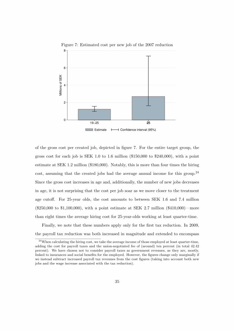
Figure 7: Estimated cost per new job of the 2007 reduction

0

2

4

6

8

Mill

ions o

f S

EK

19−25 2525

Estimate Confidence interval (95%)

of the gross cost per created job, depicted in figure 7. For the entire target group, the

gross cost for each job is SEK 1.0 to 1.6 million ($150,000 to $240,000), with a point

estimate at SEK 1.2 million ($180,000). Notably, this is more than four times the hiring

cost, assuming that the created jobs had the average annual income for this group.24

Since the gross cost increases in age and, additionally, the number of new jobs decreases

in age, it is not surprising that the cost per job soar as we move closer to the treatment

age cutoff. For 25-year olds, the cost amounts to between SEK 1.6 and 7.4 million

($250,000 to $1,100,000), with a point estimate at SEK 2.7 million ($410,000)—more

than eight times the average hiring cost for 25-year-olds working at least quarter-time.

Finally, we note that these numbers apply only for the first tax reduction. In 2009,

the payroll tax reduction was both increased in magnitude and extended to encompass

24When calculating the hiring cost, we take the average income of those employed at least quarter-time,adding the cost for payroll taxes and the union-negotiated fee of (around) ten percent (in total 42.42percent). We have chosen not to consider payroll taxes as government revenues, as they are, mostly,linked to insurances and social benefits for the employed. However, the figures change only marginally ifwe instead subtract increased payroll tax revenues from the cost figures (taking into account both newjobs and the wage increase associated with the tax reduction).

35

all individuals under 26. Although we have no useful employment estimates for this

period, we know that the gross cost almost doubled in 2009. Thus, if our results are

indicative also for the employment response of the 2009 extension, the cost per job is

likely to be significantly higher for this period than for the 2007 original tax reduction.

8 Discussion

The previous sections have painted a picture of the 2007 and 2009 payroll tax cuts as

being largely unsuccessful—the impact on youth employment was small, and the cost

per created job was high. This may seem puzzling at first glance: wages should be rigid

in the short run, so we might at least have expected a temporary employment boost.

Indeed, the wage regressions demonstrate that there were no extensive wage adaptations

that could explain the meager impact on employment. This begs the question of why

employers do not increase their hiring of young workers, despite the latter now being

significantly less expensive. In discussing potential answers to this question, we will

consider labor supply constraints and labor demand constraints, in that order.

It is, in principle, possible that the lack of employment response is caused by low labor

supply. There are many alternatives to employment for young individuals in Sweden.

Many are taking part in higher education, others spend a couple of years after high

school travelling the world. It is also possible that some of those who are formally

applying for a job are actually quite satisfied with the comfortable life of receiving

unemployment benefits while living with their parents, thus stifling the willingness to

work. These speculations are, to an extent, tested in our regressions for the subsample of

previously unemployed 25-year-olds. By restricting the sample to those registered at the

unemployment office, we disregard both the unemployed students and the globe trotters.

While the fundamental issue of weak economic incentives remain, we should diminish its

importance by studying 25-year-olds—for individuals at this age there is a strong social

36

stigma both of being unemployed and of living with one’s parents (thus the economic

incentives kick in stronger as well). The null effect for unemployed indicates that labor

supply is not the main problem. We thus conclude that the weak employment response

is more likely to be a consequence of low demand elasticity.

Turning to labor demand, we discuss a number of alternative explanations. First, it

is unlikely that employers were unaware of the new rules since the reform was covered

rather extensively in the media, both when it was ratified and later on. (The payroll

tax reductions were also criticized by the political oppositon in Sweden and, therefore,

rather intensely debated.) It is also unlikely that employers were reluctant to take any

action in the short run because they were uncertain about how persistent the new rules

would be. The reform was implemented shortly after the 2006 elections, meaning that

employers should have anticipated the new rules to be in place for at least one length

of office, which is four years in Sweden. To be sure, the extension of the payroll tax

reductions in 2009 should clearly signal that this was not a temporary policy, but even

here, we find small, or no effects.

Another possible explanation is linked to short-term capital rigidity. Since increasing

output may require long-run capital investment, the scale effects are not allowed to work

to its full extent in the short run. Thus, if firms were capacity constrained when the

lower taxes were implemented, they could not immediately make the capital investments

to accomodate more labor. The fact that the 2007 reduction was implemented in a

booming economy speaks for this explanation. But this explanation is, at the very most,

plausible only for the very short run—if this were true, we would see increasing effects

at least at the end of the period under study. Furthermore, Skedinger (2013) shows

that the effects were small also in the Swedish retail industry, where firms should be

less capacity constrained. Indeed, for this industry it is during a boom that employers

should be most willing to hire young workers, also in the short run.

A third possible explanation for the lack of large employment effects is that the wage

37

cost for the typical young worker is too high in relation to her productivity, even after

the tax cut. That is, the labor cost reduction does not compensate for the risk premium

of hiring a young, untrained, and unexperienced worker. This corresponds to a situation

where, for many firms, factor demand for young labor is at a corner solution, at zero

demand. In such a scenario, any cost-reducing measure that does not push labor costs

below the hiring threshold will have zero effect on the firm’s labor demand—i.e., the

demand elasticity will be locally zero. This explanation is corroborated by the fact that

for previously unemployed, where labor costs should correspond even less to productivity,

we find no effects at all. Conversely, when restricting the sample to individuals with

vocational training—for whom there is known to be a supply shortage—we find notably

larger effects on employment. This suggests that targeted payroll tax reductions can be

effective only if they are very selective.

It is important to stress that the figures reported in this study may not reflect net

effects on the labor market as a whole. In section 5 we describe how control group

substitution induces a substitution effect bias in all of our estimates. But negative

substitution is likely to affect also older workers in the economy—if they are similar to

the target group in terms of labor market characteristics. Thus, the larger employment

increase for 19–25 year-olds, compared to 25-year-olds, can be the result of increased

substitution with older workers. In other words, while we do find an absolute employment

increase for the target group, this may not reflect a net increase in the economy as a

whole. The share of the employment increase that is associated with a net creation of

jobs corresponds to the relative share of the scale effect (as defined in section 5), which,

unfortunately, we cannot quantify. However, it should be noted that if factor inputs

are close to perfect substitutes (e.g., low-skilled labor at different ages), there may be

large substitution effects even though the scale effect is small.25 As a consequence, it

25Indeed, in 2013 an employer of low-skilled labor stated explicitly that they only hire workers whoare subjected to the lower payroll tax. This prompted the Swedish Trade Union Confederation to suethe employer on behalf of a 35-year-old worker (Svenska Dagbladet 2013). The case has not yet been

38

is likely that our estimates grossly overestimate the number of new jobs created: partly

because the estimates overestimate the actual employment increase (due to control group

treatment spillover), partly because the actual employment increase may have been at

the expense of older workers in the economy. Similarly, the estimated cost per job,

reported in the previous section, is bound to underestimate the true cost.

9 Conclusion

This paper studies whether large-scale payroll tax reductions for employers of young

workers is an effective means to raise youth employment. In 2007–08, payroll taxes in

Sweden were cut with 11 percentage points for employers of workers at 19–25 years of

age. We estimate the effect of this substantial tax cut to be, at most, an employment

increase at around 2.7 percent. We find no employment effect of an extension of the

original reductions, implemented in 2009. Shifting of the tax cut onto workers in the

form of higher wages cannot explain the modest employment effect: the size of the wage

adjustments in the wake of the reform is small, at roughly one percent. The employment

and wage estimates in combination imply that the elasticity of demand for young workers

in Sweden is at around −0.31. Using a different metric: the estimated cost per created

job for 19–25 year-olds was SEK 1.0 to 1.6 million ($150,000 to $240,000). Since we

are likely to overestimate the employment increase, these figures are most likely overly

optimistic. We conclude that targeted payroll tax cuts are an expensive way to boost

employment for young individuals.

settled.

39

References

Anderson, P. M. and B. D. Meyer (1997). The effects of firm specific taxes and gov-

ernment mandates with an application to the u.s. unemployment insurance program.

Journal of Public Economics 65 (2), 119–145.

Anderson, P. M. and B. D. Meyer (2000). The effects of the unemployment insur-

ance payroll tax on wages, employment, claims and denials. Journal of Public Eco-

nomics 78 (1-2), 81–106.

Bennmarker, H., E. Mellander, and B. Ockert (2009). Do regional payroll tax reductions

boost employment? Labour Economics 16 (5), 480–489.

Blundell, R., M. C. Dias, C. Meghir, and J. van Reenen (2004). Evaluating the employ-

ment impact of a mandatory job search program. Journal of the European Economic

Association 2 (4), 569–606.

Bohm, P. and H. Lind (1993). Policy evaluation quality : A quasi-experimental

study of regional employment subsidies in sweden. Regional Science and Urban Eco-

nomics 23 (1), 51–65.

Edmark, K., C.-Y. Liang, E. Mork, and H. Selin (2012). Evaluation of the swedish earned

income tax credit. Working Paper Series 2012:1, IFAU - Institute for Evaluation of

Labour Market and Education Policy.

Forslund, A., L. Hensvik, O. Nordsrom Skans, and A. Westerberg (2012). Kollektivav-

talen och ungdomarnas faktiska begynnelseloner. Working Paper Series 2012:19, IFAU

- Institute for Evaluation of Labour Market and Education Policy.

Fredriksson, P. and B. Ockert (2005). Is early learning really more productive? the

effect of school starting age on school and labor market performance. IZA Discussion

Papers 1659, Institute for the Study of Labor (IZA).

40

Fredriksson, P. and R. H. Topel (2010). Wage determination and employment in sweden

since the early 1990s: Wage formation in a new setting. In R. B. Freeman, B. Swe-

denborg, and R. H. Topel (Eds.), Reforming the welfare state : recovery and beyond

in Sweden, pp. 540–559. Chicago: University of Chicago Press.

Gregg, P. (2001). The impact of youth unemployment on adult unemployment in the

ncds. The Economic Journal 111 (475), 626–653.

Gregg, P. and E. Tominey (2005). The wage scar from male youth unemployment. Labour

Economics 12 (4), 487 – 509.

Gruber, J. (1994). The incidence of mandated maternity benefits. American Economic

Review 84 (3), 622–41.

Gruber, J. (1997). The incidence of payroll taxation: Evidence from chile. Journal of

Labor Economics 15 (3), S72–101.

Hoynes, H. W., D. L. Miller, and J. Schaller (2012). Who suffers during recessions?

Working Paper 17951, National Bureau of Economic Research.

Huttunen, K., J. Pirttila, and R. Uusitalo (2013). The employment effects of low-wage

subsidies. Journal of Public Economics 97 (0), 49 – 60.

ILO (1983). Thirteenth International Conference of Labour Statisticians, Resolution

Concerning Statistics of the Economically Active Population, Employment, Unem-

ployment and Underemployment. Bulletin of Labour Statistics (1983-3), xi–xv.

Kolm, A.-S. (1998). Differentiated payroll taxes, unemployment, and welfare. Journal

of Public Economics 70 (2), 255 – 271.

Korkeamaki, O. and R. Uusitalo (2009). Employment and wage effects of a payroll-tax

cut – evidence from a regional experiment. International Tax and Public Finance 16,

753–772.

41

Kramarz, F. and T. Philippon (2001). The impact of differential payroll tax subsidies

on minimum wage employment. Journal of Public Economics 82 (1), 115–146.

Murphy, K. J. (2007). The impact of unemployment insurance taxes on wages. Labour

Economics 14 (3), 457–484.

National Mediation Office (2007). Avtalsrorelsen och lonebildningen 2007. Technical

report, Annual Report, Stockholm.

Nordstrom Skans, O. (2004). Scarring effects of the first labour market experience: A

sibling based analysis. Working Paper Series 2004:14, IFAU - Institute for Evaluation

of Labour Market and Education Policy.

Skedinger, P. (2012). Tudelad trygghet. In A. Teodorescu and L.-O. Pettersson (Eds.),

Jobben kommer och gar : behovet av trygghet bestar, pp. 114–135. Stockholm: Ekerlid.

Skedinger, P. (2013). Effects of Payroll Tax Cuts for Young Workers. Nordic Economic

Policy Review (forthcoming).

Svenska Dagbladet (2013). 35-aring for gammal for jobbet. Svenska Dagbladet,

8 October 2013. Available: http://www.svd.se/naringsliv/nyheter/sverige/

35-aring-var-for-gammal-for-jobbet_8594976.svd [Last accessed: 5 November

2013].

42

A Additional results

Table A.1: Alternative control group specifications

25 vs. 27 25 vs. 26–27 19–25 vs. 26–27

Linear Matched Linear Matched Linear Matched

DD 2005 0.002 0.002 0.002 0.002 −0.003* −0.003**(0.002) (0.002) (0.002) (0.002) (0.001) (0.001)

DD 2006 0.001 0.001 −0.000 −0.000 0.004 0.003**(0.002) (0.002) (0.001) (0.002) (0.003) (0.001)

DD 2007 0.007*** 0.007*** 0.007*** 0.007*** 0.013*** 0.013***(0.002) (0.002) (0.002) (0.002) (0.003) (0.001)

DD 2008 0.010*** 0.010*** 0.008*** 0.007*** 0.010** 0.009***(0.002) (0.002) (0.002) (0.002) (0.003) (0.001)

R2 0.10 0.11 0.10 0.10 0.11 0.12N 1,753,297 1,753,297 2,628,227 2,628,227 7,794,643 7,794,643yTG 0.59 0.59 0.59 0.59 0.52 0.52

*** p < 0.1%, ** p < 1%, * p < 5%, ’ p < 10%

Notes: Outcome is average employment status during the year (ranging from 0 to 1),yTG denotes treatment group average employment in the treatment period. All treatmenteffects are relative to the reference period 2001–04. Fixed effects included for year anddemographic characteristics. Standard errors are cluster-robust w.r.t. local labor markets(Linear) or obtained by bootstrapping with 250 replications (Matched).

43

Publication series published by IFAU – latest issues

Rapporter/Reports

2013:1 Olsson Martin ”Anställningsskydd och föräldrarelaterad frånvaro”

2013:2 Angelov Nikolay, Per Johansson and Erica Lindahl ”Det envisa könsgapet i inkomster och löner – Hur mycket kan förklaras av skillnader i familjeansvar?”

2013:3 Vikman Ulrika ”Så påverkar föräldraförsäkringen nyanlända invandrares etablering på arbets-marknaden”

2013:4 Forslund Anders, Linus Liljeberg and Leah von Trott zu Solz ”Arbetspraktik – en utvärdering och en jämförelse med arbetsmarknadsutbildning”

2013:5 Eliasson Tove ”Löneutveckling bland invandrade och infödda – betydelsen av arbetsplatser och yrken”

2013:6 Katz Katarina and Torun Österberg ”Unga invandrare – utbildning, löner och utbildnings-avkastning”

2013:7 Angelov Nikolay, Per Johansson and Erica Lindahl ”Kvinnors större föräldraansvar och högre sjukfrånvaro”

2013:8 Johansson Per, Lisa Laun and Tobias Laun ”Hälsan hos nybeviljade förtidspensionärer över tid”

2013:9 Engdahl Mattias and Olof Åslund ”Arbetsmarknadseffekter av öppna gränser”

2013:10 Bennmarker Helge, Lars Calmfors and Anna Larsson Seim ”Jobbskatteavdrag, arbetslöshets-ersättning och löner”

2013:11 Lundin Martin, Jonas Thelander and PerOla Öberg ”Det välgrundade beslutet: om kommunal beredning i kommunstyrelse, utbildnings-, arbetsmarknads- och miljöärenden”

2013:12 Liljeberg Linus, Sara Martinson and Jonas Thelander ”Jobb- och utvecklingsgarantin – Vilka deltar, vad gör de och vart leder det?”

2013:13 Avdic Daniel and Per Johansson ”Könsskillnader i preferenser för sjukfrånvaro”

2013:14 Hensvik Lena and Oskar Nordström Skans ”Hur arbetslivserfarenhet och nätverk kan förändra avkastningen på förmågor och utbildning”

2013:15 Svaleryd Helena ”Den lokala konjunkturen och egenföretagande”

2013:16 Hall Caroline ”Medförde längre och mer generella yrkesprogram en minskad risk för arbets-löshet?”

2013:17 Wondratschek Verena, Karin Edmark and Markus Frölich ”Effekter av 1992 års skolvals-reform”

2013:18 Edmark Karin and Roger Gordon ”Beskattning och val av företagsform”

2013:19 Golsteyn Bart H.H., Hans Grönqvist and Lena Lindahl ”Tidspreferenser och långsiktiga utfall”

2013:20 Hensvik Lena and Oskar Nordström Skans ”Kontakter och ungdomars arbetsmarknadsinträde”

2013:21 Dahlberg Matz, Eva Mörk and Katarina Thorén ”Jobbtorg Stockholm – resultat från en enkätundersökning”

2013:22 Sibbmark Kristina ”Arbetsmarknadspolitisk översikt 2012”

2013:23 Hedlin Maria and Magnus Åberg ”Vara med i gänget?” – Yrkessocialisation och genus i två gymnasieprogram”

2013:24 Alam Moudud, Kenneth Carling and Ola Nääs ”Har kommunala sommarjobb under gymnasieåren en positiv effekt på arbetskarriären senare i livet?”

2013:25 Lundin Andreas and Tomas Hemmingsson ”Prediktorer för arbetslöshet och förtidspension”

2013:26 Egebark Johan and Niklas Kaunitz ”Sänkta arbetsgivaravgifter för unga”

Working papers

2013:1 Nekby Lena, Peter Skogman Thoursie and Lars Vahtrik ”Examination behavior – Gender differences in preferences?”

2013:2 Olsson Martin “Employment protection and parental child care”

2013:3 Angelov Nikolay, Per Johansson and Erica Lindahl “Is the persistent gender gap in income and wages due to unequal family responsibilities?”

2013:4 Vikman Ulrika “Paid parental leave to immigrants: An obstacle to labor market entrance?”

2013:5 Pingel Ronnie and Ingeborg Waernbaum “Effects of correlated covariates on the efficiency of matching and inverse probability weighting estimators for causal inference”

2013:6 Forslund Anders, Linus Liljeberg and Leah von Trott zu Solz ”Job practice: an evaluation and a comparison with vocational labour market training programmes”

2013:7 Eliasson Tove “Decomposing immigrant wage assimilation – the role of workplaces and occupations”

2013:8 Katz Katarina and Torun Österberg “Wages of childhood immigrants in Sweden – education, returns to education and overeducation”

2013:9 Angelov Nikolay, Per Johansson and Erica Lindahl “Gender differences in sickness absence and the gender division of family responsibilities”

2013:10 Johansson Per, Lisa Laun and Tobias Laun “Screening stringency in the disability insurance program”

2013:11 Åslund Olof and Mattias Engdahl “Open borders, transport links and local labor markets”

2013:12 Bennmarker Helge, Lars Calmfors and Anna Larsson Seim “Earned income tax credits, unemployment benefits and wages: empirical evidence from Sweden”

2013:13 Avdic Daniel and Per Johansson “Gender differences in preferences for health-related absences from work”

2013:14 Lundin Martin, Oskar Nordström Skans and Pär Zetterberg “Political training as a pathway to power: the impact of participation in student union councils on candidate emergence”

2013:15 Hensvik Lena and Oskar Nordström Skans “Social networks, employee selection and labor market outcomes”

2013:16 Svaleryd Helena “Self-employment and the local business cycle”

2013:17 Hall Caroline ”Does more general education reduce the risk of future unemployment? Evidence from labor market experiences during the Great Recession”

2013:18 Sjögren Anna and Johan Vikström “How long and how much? Learning about the design of wage subsidies from policy discontinuities”

2013:19 Josephson Malin, Nina Karnehed, Erica Lindahl and Helena Persson “Intergenerational trans-misson of long-term sick leave”

2013:20 Wondratschek Verena, Karin Edmark and Markus Frölich ”The short- and long-term effects of school choice on student outcomes – evidence from a school choice reform in Sweden”

2013:21 Edmark Karin and Roger Gordon ”Taxes and the choice of organizational form by entrepre-neurs in Sweden”

2013:22 Golsteyn Bart H.H., Hans Grönqvist and Lena Lindahl ”Time preferences and lifetime outcomes”

2013:23 Hensvik Lena and Oskar Nordström Skans “Networks and youth labor market entry”

2013:24 Alam Moudud, Kenneth Carling and Ola Nääs “The effect of summer jobs on post-schooling incomes”

2013:25 Lundin Andreas and Tomas Hemmingsson “Adolescent predictors of unemployment and disability pension across the life course – a longitudinal study of selection in 49 321 Swedish men”

2013:26 van den Berg Gerard J., Arne Uhlendorff and Joachim Wolff “Sanctions for young welfare recipients”

2013:27 Egebark Johan and Niklas Kaunitz “Do payroll tax cuts raise youth employment?”

Dissertation series 2013:1 Vikman Ulrika “Benefits or work? Social programs and labor supply”