WiSe 2012 15.11.2012

Prof. Dr. A.-S. SmithDipl.-Phys. Ellen FischermeierDipl.-Phys. Matthias Sabaam Lehrstuhl für Theoretische Physik IDepartment für PhysikFriedrich-Alexander-UniversitätErlangen-Nürnberg

Theoretische Physik 2: Elektrodynamik(Prof. A.-S. Smith)

Home assignment 5

Problem5.1 Quadrupole moment

A nucleus with quadrupole moment Q finds itself in a cylindrically symmetric electric field with agradient (∂Ez/∂z)0 along the z axis at the position of the nucleus.

a) Show that the energy of quadrupole interaction is

W = −e4Q

(∂Ez∂z

)0

.

b) If it is known that Q = 2× 10−24 cm2 and that W/h is 10 MHz, where h is Planck’s constant,calculate (∂Ez/∂z)0 in units of e/a30, where a0 = }2/me2 = 0.529× 10−8 cm is the Bohr radiusin hydrogen.

c) Nuclear-charge distributions can be approximated by a constant charge-density throughout aspheroidal volume of semimajor axis a and semiminor axis b. Calculate the quadrupole momentof such a nucleus, assuming that the total charge is Ze. Given that Eu153(Z = 63) has aquadrupole moment Q = 2.5× 10−24 cm2 and a mean radius

R = (a+ b)/2 = 7× 10−13 cm,

determine the fractional difference in radius (a− b)/R.

Problem5.2 Hollow cylinder

a) A hollow right circular cylinder of radius b has its axis coincident with the z axis and itsends at z = 0 and z = L. The potential on the end faces is zero, while the potential on thecylindrical surface is given as V (φ, z). Using the appropriate separation of variables in cylindricalcoordinates, find a series solution for the potential anywhere inside the cylinder.

b) For the cylinder in part (a) the cylindrical surface is made of two equal half-cylinders, one atpotential V and the other at potential −V , so that

V (φ, z) =

{V ; −π

2 < φ < π2

−V ; π2 < φ < 3π

2 .

(i) Find the potential inside the cylinder.(ii) Assuming L� b, consider the potential at z = L/2 as a function of ρ and φ and compare

it with the two-dimensional case from Tutorial 5.3.

Problem5.3 Spherical cap

A spherical surface of radius R has charge uniformly distributed over its surface with a densityQ/(4πR2), except for a spherical cap at the north pole, defined by the cone θ ≤ α.

a) Show that the potential inside the spherical surface can be expressed as

Φ =Q

2

∞∑l=0

1

2l + 1[Pl+1(cosα)− Pl−1(cosα)]

rl

Rl+1Pl(cos θ)

where, for l = 0, Pl−1(cosα) = −1. What is the potential outside?b) Find the magnitude and the direction of the electric field at the origin.c) Discuss the limiting forms of the potential (from part a) and electric field (from part b) as the

spherical cap becomes (1) very small, and (2) so large that the area with charge on it becomesa very small cap at the south pole.

Problem5.4 Hemispherical boss

A large parallel plate capacitor is made up of two plane conducting sheets with separation D, one ofwhich has a small hemispherical boss of radius a on its inner surface (D � a). The conductor with theboss is kept at zero potential, and the other conductor is at a potential such that far from the boss theelectric field between the plates is E0.

a) Calculate the surface-charge densities at an arbitrary point on the plane and on the boss, andsketch their behavior as a function of distance (or angle).

b) Show that the total charge on the boss has the magnitude 3E0a2/4.

c) If, instead of the other conducting sheet at a different potential, a point charge q is placeddirectly above the hemispherical boss at a distance d from its center, show that the chargeinduced on the boss is

q′ = −q[1− d2 − a2

d√d2 + a2

].

Due date: Tuesday, 20.11.12

WiSe 2012 15.11.2012

Prof. Dr. A.-S. SmithDipl.-Phys. Ellen FischermeierDipl.-Phys. Matthias Sabaam Lehrstuhl für Theoretische Physik IDepartment für PhysikFriedrich-Alexander-UniversitätErlangen-Nürnberg

Theoretische Physik 2: Elektrodynamik(Prof. A.-S. Smith)

Solutions to Home assignment 5

Solution of Problem5.1 Quadrupole moment

a) In the nucleus the charge distribution has cylindrical symmetry (refer Classical Electrodynamics, byJ. D. Jackson, pages 142-143). If we choose the z-axis in the direction of the azimuthal symmetry, theonly non-vanishing terms of the quadrupole moment are the diagonal ones

Q11 = Q22 = −Q33

2

To see that we will write the non-diagonal terms of quadrupole moment in cylindrical coordinates

Qij =

∫3x

′ix

′jρe(ρ

′, z

′)ρ

′dρ

′dϕ

′dz

′

ρe = ρe(ρ′, z

′) is charge density, and ρ′ is coordinate.

Every one of the quadrupole moments inviolves integration with respect to ρ′ from 0 to 2π and sineor cosine are the functions inside the integral. That is the reason why we get 0 as solution. Diagonalterms of quadrupole moments are:

Q11 = Qxx =

∫(3ρ

′2cos2ϕ′ − (ρ

′2 + z′2))ρe(ρ

′, z

′)ρ

′dρ

′dϕ

′dz

′

=

∫(3ρ

′2sin2ρ′ − (ρ

′2 + z′2))ρe(ρ

′, z

′)ρ

′dρ

′dϕ

′dz

′= Q22 = Qyy

Q11 +Q22 +Q33 = 0

The relation betwwen the quadrupole moment Q33 and the quadrupole moment of nucleus is given bythe relation (Jackson, page 143)

Q33 = eQ

Quadrupole part of potential energy of the nucleus is

W = −1

6

∑ij

Qij(∂Ej∂xi

)0

= −1

6{Q11((

∂E1

∂x1)0 + (

∂E2

∂x2)0) +Q33(

∂E3

∂x3)0}

= −1

6{−Q11(

∂E3

∂x3)0 +Q33(

∂E3

∂x3)0}

= −1

4Q33(

∂E3

∂x3)0

= −e4Q(∂Ez∂z

)0

where we have used the equation ∇ · ~E = 0.b)

|(∂Ez∂z

)0| = 4|W |h

h

Q

a3

e2e

a3o

= 4× 1076.626× 10−27(0.529× 10−8)3e

2× 10−24(4.8× 10−10)2a30

= 0.085e

a30

c) We calculate quadrupole moment Q33 with the help of spherical coordinates

x = aη cosϕ sin θ

y = aη sinϕ sin θ

z = bη cos θ

The variable η takes values in the interval [0,1]. The Jacobian for spherical coordinates is

J(x, y, z

η, θ, ϕ) = a2bη2 sin θ

Quadrupole moment Q33 for constant charge density ρe is

Q33 = ρe

∫(3z2 − r2)dV

= ρe

∫(2b2η2 cos2 θ − a2η2 sin2 θ)a2bη2 sin θdηdϕdθ∫ 1

0η4dη

∫ π

0cos2 θ sin θdθ =

2

15∫ 1

0η4dη

∫ π

0sin3 θdθ =

4

15

Q33 =8πa2b3ρe

15− 8πa4bρe

15=

8πa2bρe15

(b2 − a2)

Volume of spheroid is

V =4π

3a2b

2

so for charge density we get

ρe =Ze

V=

3Ze

4πa2b

For quadrupole moment and quadrupole moment of nucleus we get

Q33 =2Ze

5(b− a)(b+ a)

Q =4Z

5R(b− a)

If we set a > b, the quadrupole moment of the nucleus is negative Q < 0

a− bR

=5

4

|Q|ZR2

=5× 2.5× 10−24

4× 63× (7× 10−13)2= 0.101 ≈ 10%

Solution of Problem5.2 Hollow cylinder

a) Boundary conditions for the potential (Figure 1) are

Φ(z = L) = Φ(z = 0) = 0

Φ(ρ = a) = V (ϕ, z) . (1)

Fig. 1: Upright cylinder, the bases of which are on the zero potential, whereas its sheet is on the potentialV (ϕ, z)

We are going to find the solution of the Laplace equation using the method of separation ofvariables

Φ(~x) = R(ρ)Q(ϕ)Z(z) . (2)

Upon insertion of the (2) in the Laplace equation we obtain(d2R

dρ2+

1

ρ

dR

dρ

)1

R+

1

ρ2d2Q

dϕ2

1

Q+

1

Z

d2Z

dz2= 0 . (3)

Coordinate z is appearing only in the last term so we set

1

Z

d2Z

dz2= −k2 , (4)

3

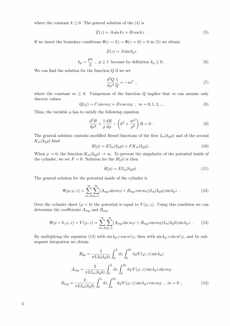
where the constant k ≥ 0. The general solution of the (4) is

Z(z) = A sin kz +B cos kz . (5)

If we insert the boundary conditions Φ(z = L) = Φ(z = 0) = 0 in (5) we obtain

Z(z) = A sin kpz

kp =pπ

L, p ≥ 1 because by definition kp ≥ 0 . (6)

We can find the solution for the function Q if we set

d2Q

dϕ2

1

Q= −m2 , (7)

where the constant m ≥ 0. Uniqueness of the function Q implies that m can assume onlydiscrete values

Q(ϕ) = C sinmϕ+D cosmϕ , m = 0, 1, 2, ... (8)

Thus, the variable ρ has to satisfy the following equation

d2R

dρ2+

1

ρ

dR

dρ−(k2 +

m2

ρ2

)R = 0 . (9)

The general solution contains modified Bessel functions of the first Im(kpρ) and of the secondKm(kpρ) kind

R(ρ) = EIm(kpρ) + FKm(kpρ) . (10)

When ρ→ 0, the function Km(kpρ)→∞. To prevent the singularity of the potential inside ofthe cylinder, we set F = 0. Solution for the R(ρ) is then

R(ρ) = EIm(kpρ) . (11)

The general solution for the potential inside of the cylinder is

Φ(ρ, ϕ, z) =∞∑m=0

∞∑p=1

(Amp sinmϕ+Bmp cosmϕ)Im(kpρ) sin kpz . (12)

Over the cylinder sheet (ρ = b) the potential is equal to V (ϕ, z). Using this condition we candetermine the coefficients Amp and Bmp.

Φ(ρ = b, ϕ, z) = V (ϕ, z) =∞∑m=0

∞∑p=1

(Amp sinmϕ+Bmp cosmϕ)Im(kpb) sin kpz . (13)

By multiplying the equation (13) with sin kp′z cosm′ϕ, then with sin kp′z sinm′ϕ, and by sub-sequent integration we obtain

B0p =1

πLI0(kpb)

∫ L

0dz

∫ 2π

0dϕV (ϕ, z) sin kpz

Amp =2

πLIm(kpb)

∫ L

0dz

∫ 2π

0dϕV (ϕ, z) sin kpz sinmϕ

Bmp =2

πLIm(kpb)

∫ L

0dz

∫ 2π

0dϕV (ϕ, z) sin kpz cosmϕ , m > 0 , (14)

4

where we used the orthogonality relations∫ L

0dz sin kp′z sin kpz =

L

2δp′p∫ 2π

0dϕ sinm′ϕ sinmϕ = πδm′m∫ 2π

0dϕ cosm′ϕ cosmϕ = πδm′m∫ 2π

0dϕ sinm′ϕ cosmϕ = 0 . (15)

By determining the coefficients in (14) the problem is solved.b) (i) In the part a) of the problem we calculated the potential inside of the cylinder of the length

L, where both bases are grounded and the cylinder sheet is on the potential V (ϕ, z)

Φ(ρ, ϕ, z) =∞∑m=0

∞∑p=1

(Amp sinmϕ+Bmp cosmϕ)Im(kpρ) sin kpz

B0p =1

πLI0(kpb)

∫ L

0dz

∫ 2π

0dϕV (ϕ, z) sin kpz

Amp =2

πLIm(kpb)

∫ L

0dz

∫ 2π

0dϕV (ϕ, z) sin kpz sinmϕ

Bmp =2

πLIm(kpb)

∫ L

0dz

∫ 2π

0dϕV (ϕ, z) sin kpz cosmϕ , m > 0 , (16)

where kp = pπ/L, p = 1, 2, ...

Fig. 2: Distribution of the potential over the cylinder.

Before we start to calculate the coefficients, observe that the distribution of the potentialon the cylinder is an even function for the transformation ϕ → −ϕ (Figure 2). Then thepotential also possesses the same symmetry, in other words, the potential is also the evenfunction in ϕ, so the coefficients Amp = 0. Coefficients Bmp are equal to

B0p =V

πLI0(kpb)

(∫ L

0dz sin kpz

)(∫ π/2

−π/2dϕ−

∫ 3π/2

π/2dϕ

)= 0 (17)

5

Bmp =2V

πLIm(kpb)

(∫ L

0dz sin kpz

)(∫ π/2

−π/2cosmϕdϕ−

∫ 3π/2

π/2cosmϕdϕ

)

=2V

πLIm(kpb)

[− 1

kp(cos kpL− 1)

]{2

msin(mπ

2

)− 1

m

[sin

(3mπ

2

)− sin

(mπ2

)]}=

2V

π2Im(kpb)

1

mp[1− (−1)p]

[3 sin

(mπ2

)− sin

(3mπ

2

)]. (18)

Using the relations for the transformation of the sum and difference of the sine functioninto product we obtain

3 sin(mπ

2

)− sin

(3mπ

2

)= 2 sin

(mπ2

)+

[sin(mπ

2

)− sin

(3mπ

2

)]= 2 sin

(mπ2

)− 2 sin

(mπ2

)cosmπ

= 2 sin(mπ

2

)[1− (−1)m] . (19)

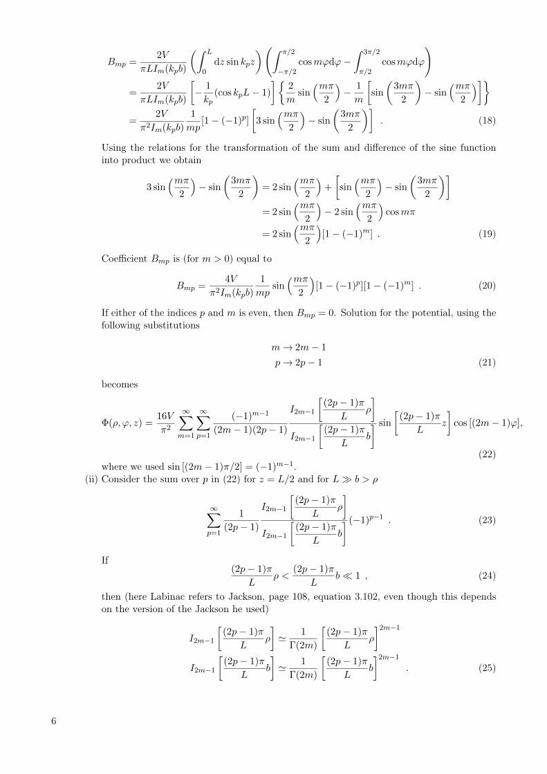
Coefficient Bmp is (for m > 0) equal to

Bmp =4V

π2Im(kpb)

1

mpsin(mπ

2

)[1− (−1)p][1− (−1)m] . (20)

If either of the indices p and m is even, then Bmp = 0. Solution for the potential, using thefollowing substitutions

m→ 2m− 1

p→ 2p− 1 (21)

becomes

Φ(ρ, ϕ, z) =16V

π2

∞∑m=1

∞∑p=1

(−1)m−1

(2m− 1)(2p− 1)

I2m−1

[(2p− 1)π

Lρ

]I2m−1

[(2p− 1)π

Lb

] sin

[(2p− 1)π

Lz

]cos [(2m− 1)ϕ],

(22)where we used sin [(2m− 1)π/2] = (−1)m−1.

(ii) Consider the sum over p in (22) for z = L/2 and for L� b > ρ

∞∑p=1

1

(2p− 1)

I2m−1

[(2p− 1)π

Lρ

]I2m−1

[(2p− 1)π

Lb

] (−1)p−1 . (23)

If(2p− 1)π

Lρ <

(2p− 1)π

Lb� 1 , (24)

then (here Labinac refers to Jackson, page 108, equation 3.102, even though this dependson the version of the Jackson he used)

I2m−1

[(2p− 1)π

Lρ

]' 1

Γ(2m)

[(2p− 1)π

Lρ

]2m−1I2m−1

[(2p− 1)π

Lb

]' 1

Γ(2m)

[(2p− 1)π

Lb

]2m−1. (25)

6

Sum over the index p becomes(ρb

)2m−1 ∞∑p=1

(−1)p−1

(2p− 1)=(ρb

)2m−1(1− 1

3+

1

5− ...

)=π

4

(ρb

)2m−1. (26)

In other words, sum over p gives the result (26) when L→∞ because then for every finitep the condition (24) is satisfied. In this limit the potential is

Φ(ρ, ϕ, z) =4V

π

∞∑m=1

(−1)m−1

(2m− 1)

(ρb

)2m−1cos [(2m− 1)ϕ] . (27)

If in the Tutorial 5.3 we put V2 = −V1 = −V , we obtain exactly this expression for thepotential.

Solution of Problem5.3 Spherical cap

a) The configuration is shown in Figure 3.

Fig. 3: Configuration in the problem.

From the given conditions we know that thecharge-density is azimuthaly symmetric andsatisfies

σ(θ) =

{0 , 0 ≤ θ ≤ αQ/(4πR2) , α ≤ θ ≤ π

and we expect that the potential has the forms

Φin(r, θ) =

∞∑l=0

Al rlPl(cos θ) inside the sphere

Φout(r, θ) =

∞∑l=0

Bl r−(l+1)Pl(cos θ) outside the sphere .

The boundary conditions for the sphere r = R are

Φin(r, θ) = Φout(r, θ) (28)

( ~Eout − ~Ein)·~n∣∣∣r=R

= 4πσ(θ) (29)

From the boundary condition (28) we get

∞∑l=0

Al RlPl(cos θ) =

∞∑l=0

Bl R−(l+1)Pl(cos θ)

⇒Al Rl = Bl R

−(l+1) .

The secondary boundary condition gives

~n = ~er

( ~Eout − ~Ein)∣∣∣r=R

= 4πσ(θ) (30)

7

For the L.H.S. in (30) we can write(− ∂Φout

∂r+∂Φin

∂r

)∣∣∣∣r=R

=

∞∑l=0

[(l + 1)BlR

−(l+2) + lAlRl−1]Pl(cos θ)

⇒∞∑l=0

[(l + 1)BlR

−(l+2) + lAlRl−1]Pl(cos θ) = 4πσ(θ)

∖× Pl′(cos θ) sin θ

∖∫ π

0dθ

∞∑l=0

[(l + 1)BlR

−(l+2) + lAlRl−1] ∫ π

0Pl(cos θ)Pl′(cos θ) sin θ dθ = 4π

∫ π

0σ(θ)Pl′(cos θ) sin θ dθ

From the orthogonality relation we know∫ π

0Pl′(cos θ)Pl(cos θ) sin θ dθ =

2

2l + 1δl′l .

Second integral ∫ π

0σ(θ)Pl(cos θ) sin θ dθ =

Q

4πR2

∫ π

αPl(cos θ) sin θ dθ (31)

Changing the variable cos θ = x and using the relation

dPl+1

dx− dPl−1

dx− (2l + 1)Pl = 0 , l ≥ 1

the integral (31) becomes∫ π

0σ(θ)Pl(cos θ) sin θ dθ =

Q

4πR2

1

2l + 1

∫ cosα

−1

[dPl+1(x)

dx− dPl−1(x)

dx

]dx , l ≥ 1

=Q

4πR2

1

2l + 1[Pl+1(cosα)− Pl−1(cosα)]

⇒ (l + 1)BlR−(l+2) + lAlR

l−1 =Q

2R2[Pl+1(cosα)− Pl−1(cosα)] (32)

For l = 0 ∫ π

αPl(cos θ) sin θ dθ = cosα+ 1 . (33)

If we require that (32) is also valid for l = 0 and in the accordance with (33) we take as thedefinition P−1(cosα) = −1. The coefficients Al and Bl are then equal to

Al =Q

2Rl+1

1

2l + 1[Pl+1(cosα)− Pl−1(cosα)] (34)

Bl =Q

2

Rl

2l + 1[Pl+1(cosα)− Pl−1(cosα)] . (35)

Finally, the potential solution reads

Φin =Q

2

∞∑l=0

1

2l + 1[Pl+1(cosα)− Pl−1(cosα)]

rl

Rl+1Pl(cos θ) (36)

Φout =Q

2

∞∑l=0

1

2l + 1[Pl+1(cosα)− Pl−1(cosα)]

Rl

Rl+1Pl(cos θ) . (37)

8

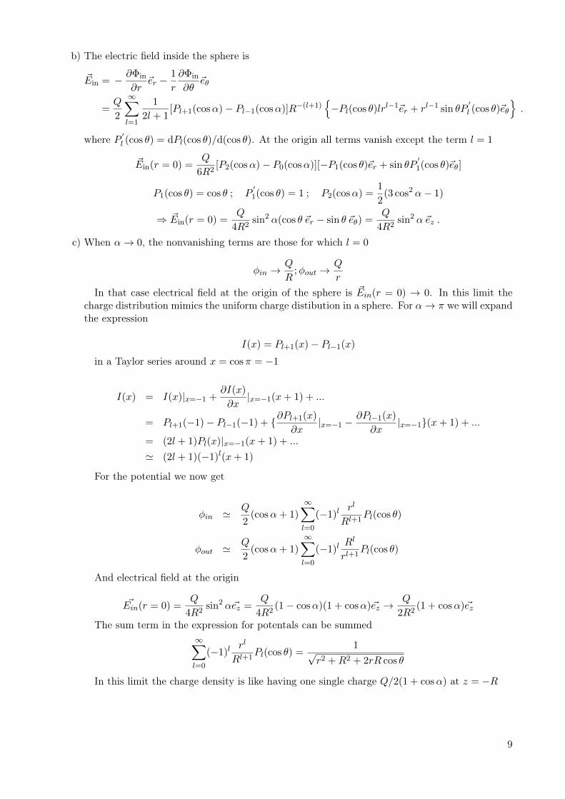
b) The electric field inside the sphere is

~Ein = − ∂Φin

∂r~er −

1

r

∂Φin

∂θ~eθ

=Q

2

∞∑l=1

1

2l + 1[Pl+1(cosα)− Pl−1(cosα)]R−(l+1)

{−Pl(cos θ)lrl−1~er + rl−1 sin θP

′l (cos θ)~eθ

}.

where P ′l (cos θ) = dPl(cos θ)/d(cos θ). At the origin all terms vanish except the term l = 1

~Ein(r = 0) =Q

6R2[P2(cosα)− P0(cosα)][−P1(cos θ)~er + sin θP

′1(cos θ)~eθ]

P1(cos θ) = cos θ ; P′1(cos θ) = 1 ; P2(cosα) =

1

2(3 cos2 α− 1)

⇒ ~Ein(r = 0) =Q

4R2sin2 α(cos θ ~er − sin θ ~eθ) =

Q

4R2sin2 α ~ez .

c) When α→ 0, the nonvanishing terms are those for which l = 0

φin →Q

R;φout →

Q

r

In that case electrical field at the origin of the sphere is ~Ein(r = 0) → 0. In this limit thecharge distribution mimics the uniform charge distibution in a sphere. For α→ π we will expandthe expression

I(x) = Pl+1(x)− Pl−1(x)

in a Taylor series around x = cosπ = −1

I(x) = I(x)|x=−1 +∂I(x)

∂x|x=−1(x+ 1) + ...

= Pl+1(−1)− Pl−1(−1) + {∂Pl+1(x)

∂x|x=−1 −

∂Pl−1(x)

∂x|x=−1}(x+ 1) + ...

= (2l + 1)Pl(x)|x=−1(x+ 1) + ...

' (2l + 1)(−1)l(x+ 1)

For the potential we now get

φin ' Q

2(cosα+ 1)

∞∑l=0

(−1)lrl

Rl+1Pl(cos θ)

φout 'Q

2(cosα+ 1)

∞∑l=0

(−1)lRl

rl+1Pl(cos θ)

And electrical field at the origin

~Ein(r = 0) =Q

4R2sin2 α~ez =

Q

4R2(1− cosα)(1 + cosα)~ez →

Q

2R2(1 + cosα)~ez

The sum term in the expression for potentals can be summed∞∑l=0

(−1)lrl

Rl+1Pl(cos θ) =

1√r2 +R2 + 2rR cos θ

In this limit the charge density is like having one single charge Q/2(1 + cosα) at z = −R

9

Solution of Problem5.4 Hemispherical boss

a) Our aim will be to find a potential which satisfies all the boundary conditions, as that will indeedbe the potential for the given problem. To find this potential, we will first find the potential fora somewhat easier problem, and then tweak it until it satisfies all the boundary conditions ofthe original problem.So, let us look at the following auxiliary problem: a charge −q is positioned at a distance R

on the z-axis from the origin in front of the conducting sheet which has a small hemisphericalboss of radius a. Let us calculate the potential in the part of the space where r ≥ a and θ ≤ π/2(Figure 1), where r and θ are as in the usual spherical coordinates.Since such a sheet containing a spherical boss is suggestive of a hemi-sphere stuck on to

a plane, we can try to solve this problem by combining the approaches using the method ofimages for the case of a plane and for that of a sphere. So let us first consider the plane, andposition the image charge q′ = q at the point z′ = −R. Then the plane is at zero potential.However, the boss is not. So let us now position a second image charge q′′ = qa/R at the pointz′′ = a2/R. Now the plane is not at zero potential anymore, so let us position another imagecharge q′′′ = −q′′ = −qa/R at the point z′′′ = −z′′ = −a2/R. The total potential is equal tothe sum of the potentials of the charge −q and the three image charges

Fig. 4: A point charge near a grounded, conducting sheet with a hemispherical boss.

Φs(~r) =q

(r2 +R2 + 2rR cos θ)1/2− q

(r2 +R2 − 2rR cos θ)1/2

+−aq

R

(r2 +

a4

R2+

2a2r

Rcos θ

)1/2+

aq

R

(r2 +

a4

R2− 2a2r

Rcos θ

)1/2.

At last, the boundary coditions for this auxiliary problem are satisfied: for both the planarand the boss part of the sheet, Φs(~r) = 0 (as can easily be verified).

This potential Φs(~r) is not the solution to the original problem, as it does not satisfy thecondition that far away from the sheet, the electric field is constant at E0 (in other words, the

10

condition that limr→∞

Φ(~r) = −E0z = −E0r cos θ). So now we try to tweak Φs(~r) a bit. So letR→∞. Then, Φs(~r) can be expanded as

Φs(~r) =q

R

[1− r2

2R2− r

Rcos θ − 1 +

r2

2R2− r

Rcos θ

]+ ...

− qarR

[1− a4

2r2R2− a2

rRcos θ − 1 +

a4

2r2R2− a2

rRcos θ

]+ ...

Φs(~r) ' −2qr

R2cos θ +

2qa3

r2R2cos θ = −2q

R

(1− a3

r3

)r

Rcos θ = −E0

(r − a3

r2

)cos θ

where E0 :=2q

R2= constant.

Hence, as r →∞, Φs(~r)→ −E0 r cos θ, as desired. Therefore, Φs(~r) = Φ(~r) = −E0

(r − a3

r2

)cos θ

is the desired potential.

Note that, physically, E0 =2q

R2is the magnitude of an electric field between two infinite hemi-

spherical (of radius R → ∞) sheets over which a surface charge σ =q

2πR2has been smeared

(because, as R → ∞, these hemi-spherical sheets together form a parallel plate capacitor,

between the plates of which we know the electric field to be E0 = 4πσ =2q

R2). Thus, having

found the potential, we can now calculate the electric field

~E = −~∇Φ = −∂Φ

∂r~er −

1

r

∂Φ

∂θ~eθ = E0 cos θ

(1 + 2

a3

r3

)~er − E0 sin θ

(1− a3

r3

)~eθ .

Now, finally, we can calculate the surface charge density on the planar and the boss part

σp ≡ σplanar =1

4π~E · ~ez

∣∣∣∣θ=π/2

= −E0

4π

(1− a3

r3

)sin θ~eθ · ~ez

∣∣∣∣θ=π/2

=E0

4π

(1− a3

r3

)because in the planar part of the surface of interest ~er · ~ez = 0 and ~eθ · ~ez = −1.

σb ≡ σboss =1

4π~E · ~er

∣∣∣∣r=a

=3

4πE0 cos θ .

The surface charge densities on the boss and the planar part are shown in the figures 3 and 4,respectively.Note: The surface charge density on the boss part is the same as the one found for the sphere

in the uniform field (see homework, Problem 4.2 b).

Fig. 5: Surface charge density on the boss. Fig. 6: Surface charge density on the planar part.

11

b) The total charge on the boss is

Qb =

∫ 2π

0dϕ

∫ π/2

0dθ sin θa2σb =

3E0a2

2

∫ π/2

0dθ sin θ cos θ =

3E0a2

4.

c) We have already found the potential for this configuration in the ‘auxiliary problem’ of part a),with the only difference being that here −q and R are replaced by q and d, respectively. So,making the following changes in Φs(~r) from part a),

q → − qR→ d,

we get

Φs(~r) = − q

(r2 + d2 + 2rd cos θ)1/2+

q

(r2 + d2 − 2rd cos θ)1/2

+aq

d

(r2 +

a4

d2+

2a2r

dcos θ

)1/2− aq

d

(r2 +

a4

d2− 2a2r

dcos θ

)1/2.

The surface charge density on the boss is

σ =1

4π~E · ~er

∣∣∣∣r=a

= − 1

4π

∂Φ

∂r

∣∣∣∣r=a

=q(d2 − a2

)4πa

[1

(a2 + d2 + 2ad cos θ)3/2− 1

(a2 + d2 − 2ad cos θ)3/2

].

In the calculation of the induced charge on the boss, integrals of the following form appear∫ π/2

0

sin θdθ

(a2 + d2 ± 2ad cos θ)3/2= ∓ 1

ad

(1

d± a− 1

(a2 + d2)1/2

).

The induced charge on the boss is then

q′ =

∫ 2π

0dϕ

∫ π/2

0dθ sin θa2σ(θ)

= −qa(d2 − a2

)2

[1

ad

(1

d+ a− 1

(a2 + d2)1/2

)+

1

ad

(1

d− a− 1

(a2 + d2)1/2

)]

=q(d2 − a2

)2d

[2d

d2 − a2− 2

(a2 + d2)1/2

]= −q

[1− d2 − a2

d (d2 + a2)1/2

].

12