Towards Active Car Body Suspension in Railway Vehicles JESSICA FAGERLUND
124
Towards Active Car Body Suspension in Railway Vehicles JESSICA FAGERLUND Department of Signals and Systems CHALMERS UNIVERSITY OF TECHNOLOGY G¨ oteborg, Sweden 2009
Transcript of Towards Active Car Body Suspension in Railway Vehicles JESSICA FAGERLUND
Towards Active Car Body Suspensionin Railway Vehicles
JESSICA FAGERLUND
Department of Signals and SystemsCHALMERS UNIVERSITY OF TECHNOLOGY
Goteborg, Sweden 2009


THESIS FOR THE DEGREE OF LICENTIATE OF ENGINEERING
Towards Active Car Body Suspensionin Railway Vehicles
JESSICA FAGERLUND
Department of Signals and SystemsCHALMERS UNIVERSITY OF TECHNOLOGY
Goteborg, Sweden 2009

Towards Active Car Body Suspension in Railway Vehicles
JESSICA FAGERLUND
Technical Report No R009/2009ISSN 1403-266X
Department of Signals and SystemsMechatronics Research GroupChalmers University of TechnologySE-412 96 Goteborg, SwedenTelephone +46 (0) 31 772 10 00
c© 2009 Jessica FagerlundAll rights reserved
Printed by Chalmers ReproserviceGoteborg, Sweden 2009
Typeset by the author with the LATEX Documentation System

abstractTowards Active Car Body Suspension in Railway VehiclesJessica Fagerlund
Department of Signals and SystemsChalmers University of Technology
Today, most railway suspension systems are passive. The most wide-spread exception isactive car body tilt systems, which are mounted in some high-speed trains. Replacing someof the passive suspension components with active could reduce the weight and cost of thevehicle. It may also improve passenger comfort without increasing the deflections withinthe suspension, or, similarly, allow the vehicle to be run at higher speeds or on less smoothtracks, with comfort and deflection kept at today’s levels.
This thesis deals with background studies of a model of a railway vehicle, aiming to-wards actively controlling its vertical secondary suspension, i.e. the part of the suspensionthat is fitted vertically between the bogie frame and the car body.
First, some requirements on the actuator, e.g. maximum forces, are studied, for somecases of replacing passive components with active. Those cases are: removing the anti-rollbars, removing the pneumatic systems of the air-spring, and both combined, in all casesadding 2 actuators in the vertical direction for each bogie. The forces the actuators have tobe able to deliver are high, but still within reason to implement.
Also, the possibility to use a single-input single-output (SISO) control design is studied.It is found that neither input/output pairing, nor using stationary decoupling matrices, givesany promising results that a SISO control design could be based on. The coupling betweenthe inputs and outputs is found to be both very high, and very frequency dependent.
To make multiple-input multiple-output (MIMO) control design a feasible choice, theoriginal nonlinear model with 330 states is linearized, and different methods of reducing thismodel are studied. A model reduction algorithm was developed, that was better suited tothis problem than the two standard methods it was compared to. The new algorithm is bothless computationally demanding, and for this model produces reduced models, that havegain curves that are closer to those of the full linear model, within the interesting frequencyregion.
Finally, an attempt is made at designing a linear quadratic (LQ) control, and the difficul-ties with that control strategy on this particular model are discussed.
Additional work is needed to fully understand the model, and to find a control law thatoffers an advantage over the fully passive system.
KEYWORDS: Active suspension, Decoupling, MIMO systems, Model reduction, LQ control,Railway vehicles
iii

iv

acknowledgments
I want to thank my supervisor and examiner, Jonas Sjoberg, as well as Thomas Abra-hamsson, who was my co-supervisor during parts of the project. Thank you Thomas Abra-hamsson, Jonas Sjoberg, and Tomas McKelvey for initiating the project.
Thanks to Bombardier Transportation and the center of excellence CHARMEC for spon-soring the work in this thesis, and to Bombardier Transportation for providing me with amodel of a train.
Thank you Madeleine Persson and Lars Borjesson, and other administrative and techni-cal staff, for help within those areas.
Finally, I want to thank my present and former colleagues and superiors, and Anna-KarinChristiansson, for valuable discussions on and off topic.
Goteborg, May 2009Jessica Fagerlund
v

vi

contents
abstract . . . . . . . . . . . . . . . . . . . . . . . . . . . . . . . . . . . . . . . iiiacknowledgments . . . . . . . . . . . . . . . . . . . . . . . . . . . . . . . . . . vcontents . . . . . . . . . . . . . . . . . . . . . . . . . . . . . . . . . . . . . . . vii
chapters
chapter i: introduction 3
1.1 Main Contributions . . . . . . . . . . . . . . . . . . . . . . . . . . . . . . 31.2 Publications . . . . . . . . . . . . . . . . . . . . . . . . . . . . . . . . . . 31.3 Thesis Outline . . . . . . . . . . . . . . . . . . . . . . . . . . . . . . . . . 4
chapter ii: background theory 5
2.1 Introduction to Railway Vehicles . . . . . . . . . . . . . . . . . . . . . . . 52.1.1 Suspension . . . . . . . . . . . . . . . . . . . . . . . . . . . . . . 5
2.2 Active Suspension in Theory and Practice - Other Research . . . . . . . . . 62.3 Human Sensitivity for Accelerations at Different Frequencies . . . . . . . . 7
2.3.1 Ride index . . . . . . . . . . . . . . . . . . . . . . . . . . . . . . 7
chapter iii: research objective, methodology and thesis structure 13
3.1 Research Objective . . . . . . . . . . . . . . . . . . . . . . . . . . . . . . 133.1.1 Evaluation Criteria . . . . . . . . . . . . . . . . . . . . . . . . . . 13
3.2 General Methods . . . . . . . . . . . . . . . . . . . . . . . . . . . . . . . 143.2.1 Software Tools . . . . . . . . . . . . . . . . . . . . . . . . . . . . 143.2.2 Linearization . . . . . . . . . . . . . . . . . . . . . . . . . . . . . 14
3.3 Work Flow and Thesis Structure . . . . . . . . . . . . . . . . . . . . . . . 14
chapter iv: model 17
4.1 Model Structure . . . . . . . . . . . . . . . . . . . . . . . . . . . . . . . . 174.1.1 Vehicle . . . . . . . . . . . . . . . . . . . . . . . . . . . . . . . . 174.1.2 Active Suspension . . . . . . . . . . . . . . . . . . . . . . . . . . 174.1.3 Inputs and Outputs . . . . . . . . . . . . . . . . . . . . . . . . . . 17
4.2 Measured Input Data . . . . . . . . . . . . . . . . . . . . . . . . . . . . . 194.2.1 Track Irregularities in Spatial Domain . . . . . . . . . . . . . . . . 194.2.2 Track Irregularities in Frequency Domain . . . . . . . . . . . . . . 19
chapter v: feasibility considerations 25
vii

5.1 Background Theory . . . . . . . . . . . . . . . . . . . . . . . . . . . . . . 255.1.1 Railway Vehicle . . . . . . . . . . . . . . . . . . . . . . . . . . . 255.1.2 Actuators . . . . . . . . . . . . . . . . . . . . . . . . . . . . . . . 26
5.2 Quasi-Static Analysis . . . . . . . . . . . . . . . . . . . . . . . . . . . . . 265.2.1 Considered Scenarios . . . . . . . . . . . . . . . . . . . . . . . . . 265.2.2 Force to Control Roll, Passive Simulations (Scenario 1) . . . . . . . 275.2.3 Force to Control Roll, Carbody Parallel with Bogie (Scenario 1) . . 285.2.4 Air-Spring Deviation from Equilibrium (Scenario 2) . . . . . . . . 305.2.5 Active Roll and Level Control (Scenario 3) . . . . . . . . . . . . . 30
5.3 Dynamic Simulations . . . . . . . . . . . . . . . . . . . . . . . . . . . . . 305.3.1 Simulated Cases . . . . . . . . . . . . . . . . . . . . . . . . . . . 315.3.2 Simulation Results . . . . . . . . . . . . . . . . . . . . . . . . . . 32
5.4 Concluding Remarks . . . . . . . . . . . . . . . . . . . . . . . . . . . . . 33
chapter vi: frequency range for linear model validity 376.1 Comparison of Same Transfer Function Obtained in Different Ways . . . . 376.2 Gain Plots Compared to Physical Insight . . . . . . . . . . . . . . . . . . . 376.3 Comparison with Nonlinear Simulations . . . . . . . . . . . . . . . . . . . 386.4 Concluding Remarks . . . . . . . . . . . . . . . . . . . . . . . . . . . . . 39
chapter vii: coupling between inputs and outputs 477.1 Background Theory . . . . . . . . . . . . . . . . . . . . . . . . . . . . . . 47
7.1.1 Relative Gain Array . . . . . . . . . . . . . . . . . . . . . . . . . 477.1.2 The Pairing Problem . . . . . . . . . . . . . . . . . . . . . . . . . 487.1.3 Decoupling . . . . . . . . . . . . . . . . . . . . . . . . . . . . . . 48
7.2 Signal Coupling and Pairing . . . . . . . . . . . . . . . . . . . . . . . . . 487.2.1 Gain Plots . . . . . . . . . . . . . . . . . . . . . . . . . . . . . . . 497.2.2 Relative Gain Array . . . . . . . . . . . . . . . . . . . . . . . . . 49
7.3 Decoupling . . . . . . . . . . . . . . . . . . . . . . . . . . . . . . . . . . 527.4 Concluding Remarks . . . . . . . . . . . . . . . . . . . . . . . . . . . . . 54
chapter viii: model reduction 618.1 Background Theory . . . . . . . . . . . . . . . . . . . . . . . . . . . . . . 61
8.1.1 State Transform . . . . . . . . . . . . . . . . . . . . . . . . . . . . 628.1.2 Diagonalization . . . . . . . . . . . . . . . . . . . . . . . . . . . . 628.1.3 Controllability and Observability . . . . . . . . . . . . . . . . . . 628.1.4 Balanced Realization . . . . . . . . . . . . . . . . . . . . . . . . . 628.1.5 Softwares for Model Simplification . . . . . . . . . . . . . . . . . 62
8.2 Evaluation Method . . . . . . . . . . . . . . . . . . . . . . . . . . . . . . 638.3 Methods of Model Reduction . . . . . . . . . . . . . . . . . . . . . . . . . 64
8.3.1 Preparatory Manipulations . . . . . . . . . . . . . . . . . . . . . . 648.3.2 Tailored Algorithm . . . . . . . . . . . . . . . . . . . . . . . . . . 658.3.3 Commercial Software . . . . . . . . . . . . . . . . . . . . . . . . 68
8.4 Comparisons and Conclusions . . . . . . . . . . . . . . . . . . . . . . . . 698.4.1 Bode Plot Comparisons . . . . . . . . . . . . . . . . . . . . . . . 698.4.2 Advantages with Each Method . . . . . . . . . . . . . . . . . . . . 698.4.3 Concluding Remarks . . . . . . . . . . . . . . . . . . . . . . . . . 70
viii

chapter ix: linear quadratic (lq) control design 819.1 Background Theory . . . . . . . . . . . . . . . . . . . . . . . . . . . . . . 81
9.1.1 Detectability and Stabilizability . . . . . . . . . . . . . . . . . . . 819.1.2 Linear Quadratic Control . . . . . . . . . . . . . . . . . . . . . . . 819.1.3 State Observer . . . . . . . . . . . . . . . . . . . . . . . . . . . . 82
9.2 Inputs and Outputs . . . . . . . . . . . . . . . . . . . . . . . . . . . . . . 829.2.1 Disturbances (Inputs) . . . . . . . . . . . . . . . . . . . . . . . . . 829.2.2 Evaluation (Outputs) . . . . . . . . . . . . . . . . . . . . . . . . . 83
9.3 Control . . . . . . . . . . . . . . . . . . . . . . . . . . . . . . . . . . . . 839.3.1 Outputs as Criterion Based on State Space Matrices . . . . . . . . . 839.3.2 Altering Output Penalty . . . . . . . . . . . . . . . . . . . . . . . 869.3.3 LQ With Optimal Feed Forward . . . . . . . . . . . . . . . . . . . 86
9.4 Concluding Remarks . . . . . . . . . . . . . . . . . . . . . . . . . . . . . 87
chapter x: concluding remarks 9110.1 Future Work . . . . . . . . . . . . . . . . . . . . . . . . . . . . . . . . . . 91
appendices
appendix a: passenger model 95
appendix b: disturbance dynamics modeling by state expansion 97
appendix c: single transfer function derived from a diagonal mimo system 101
appendix d: numerical results from feasibility chapter 103D.1 Forces in Anti-Roll Bar and Damper . . . . . . . . . . . . . . . . . . . . . 103D.2 Ideal Power Dissipation in Anti-Roll Bar and Damper . . . . . . . . . . . . 105D.3 Passenger Comfort . . . . . . . . . . . . . . . . . . . . . . . . . . . . . . 106D.4 Secondary Suspension Deflection . . . . . . . . . . . . . . . . . . . . . . . 107D.5 Secondary Suspension Roll . . . . . . . . . . . . . . . . . . . . . . . . . . 107
references
bibliography 111
ix

x

chapters


chapter i
introduction
Today, most railway suspension systems are passive. The most wide-spread exception isactive car body tilt systems, which are mounted in some high-speed trains, (Zolotas, Pearsonand Goodall 2006). Replacing some of the passive suspension components with active couldreduce the weight and cost of the vehicle, (Agren 2004–2005). It may also improve passengercomfort without increasing the deflections within the suspension, or, similarly, allow thevehicle to be run at higher speeds or on less smooth tracks, with comfort and deflection keptat today’s levels, (Goodall and Mei 2006).
This thesis is a preliminary study, dealing with the questions if it is reasonable to use ac-tive secondary suspension, and investigating further which issues that needs to be addressedfor the developing of a control strategy.
1.1 Main Contributions
• Estimation of requirements on actuators in Chapter 5.
• Studies of coupling and decoupling in Chapter 7.
• Development of a model reduction technique in Chapter 8.
• Pointing out issues with linear quadratic control for this application in Chapter 9.
1.2 Publications
• Jessica Fagerlund, Jonas Sjoberg and Thomas Abrahamsson: Passive Railway CarSecondary Suspension - Force, Power, Deflection, Roll and Comfort, Technical Report,Chalmers University of Technology, 2005.
• Jessica Fagerlund, Jonas Sjoberg and Thomas Abrahamsson: Briefly on Passive Rail-way Car Secondary Suspension - Force, Power, Deflection, Roll and Comfort, Meka-tronikmote (Mechatronics Conference), Halmstad, November 2005.
• Jessica Fagerlund, Jonas Sjoberg, Active secondary suspension in railway vehicles, S2Research Day - Poster Exhibition Abstracts, p. 12, Chalmers: Department of Signalsand Systems, October 2008.
The conference paper is a significantly abbreviated version of the internal report. Theinternal report makes up the basis for Chapter 5, Appendix A, and Appendix D, as well as

4 1. Introduction
parts of Chapter 2 and Chapter 4. The poster abstract briefly introduces the work in thisthesis.
1.3 Thesis Outline
Chapter 2 gives a brief overview of background theory regarding railway vehicles in generalas well as comfort calculations. In Chapter 3 the research objective is stated, the method isdescribed, and the flow between the chapters is described in more detail than here. Chapter 4describes the particular model used in this thesis. Chapter 5 deals with the question if it isat all reasonable to use actuators in the vertical secondary part, by estimating what would berequired by the actuators. In Chapter 6 deals with if the linear model used is adequate forthe task. In Chapter 7, 8, and 9 analysis and preparations regarding control laws are carriedout. In those chapters, Chapter 7 deals with whether SISO design is reasonable, 8 deals withmodel reduction, which is necessary for the use of state feedback, and 9 deals with issueswith LQ design. Finally, conclusions and recommendations for future work are found inChapter 10.
chapter ii
background theory
This chapter introduces the reader to some generally known facts about railway vehicles,active suspension, and how to calculate ride comfort. Other algorithms, that are only used ina single chapter, are introduced in the chapters they are used.
2.1 Introduction to Railway Vehicles
This section offers a very brief introduction to railway vehicles. Significantly more detaileddescriptions can be found in for example (Andersson and Berg 1999) and (Andersson, Bergand Stichel 2004).
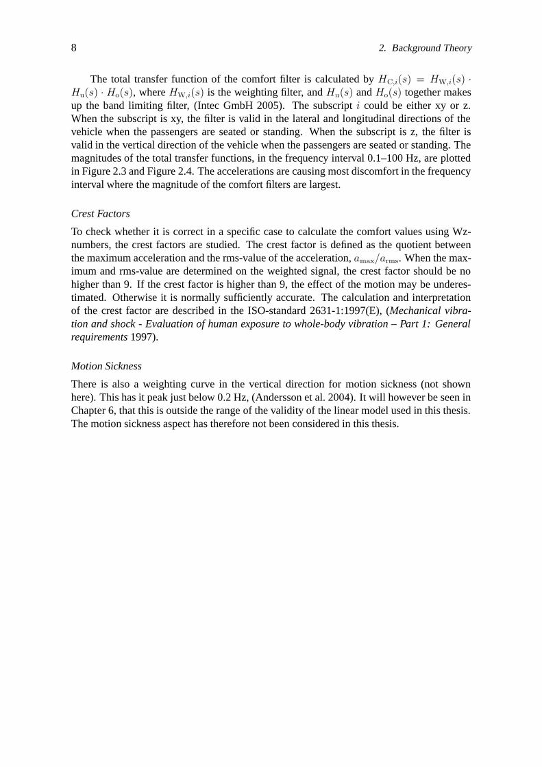
Railway vehicles are guided by a rail. In the case studied in this thesis, wheels of steelare rolling on steel rails. This is also by far the most common technique for rail vehiclesin the world, (Andersson and Berg 1999). By using this technique, the vehicle is generallyautomatically steered. (The exception is if the wheel axle is removed and the wheels individ-ually steered.) The steering works in the following way: The wheels are shaped in a way thatmakes the running circle longer if the wheel is moving outwards on the rails. At the sametime the wheel on the other side moves inwards (assuming the distance between the rails,called gauge, is constant). This way the wheels on the left and the right side travel differentfar during one revolution, and this way the wheelset is steering towards centering over therails, see Figure 2.1.
In many cases, including in this thesis, the wheelsets are connected (by a suspension)two by two to a bogie (wheel truck). The bogies are then connected (by a suspension) tothe car body. Using bogies improves the curving performance and decreases the risk ofderailment, compared to using a suspension directly between the wheelsets and car body,(Andersson et al. 2004). Also, using bogies makes it possible to reduce car body vibrationsas well as wheel-rail forces, (Andersson et al. 2004).
2.1.1 Suspension
This subsection briefly introduces the suspension areas the reader needs to be familiar withto understand this thesis.
In general, the suspension is the set of elastic elements (springs), dampers and associatedcomponents which connect the wheelsets to the car body, (Orlova and Boronenko 2006). Thesuspension can be divided into primary and secondary suspension. The primary suspensionis the suspension between the wheelset and the bogie frame. The secondary suspension isthe suspension between the bogie frame and the car body, (Andersson and Berg 1999). See

6 2. Background Theory
Figure 4.1. The springs are used to equalize the vertical loads between the wheels, stabilizethe motion of the vehicle on the track, and to reduce the dynamic forces and accelerationsdue to track irregularities, (Orlova and Boronenko 2006). Dampers are used to dampen theoscillations in the suspension, (Orlova and Boronenko 2006).
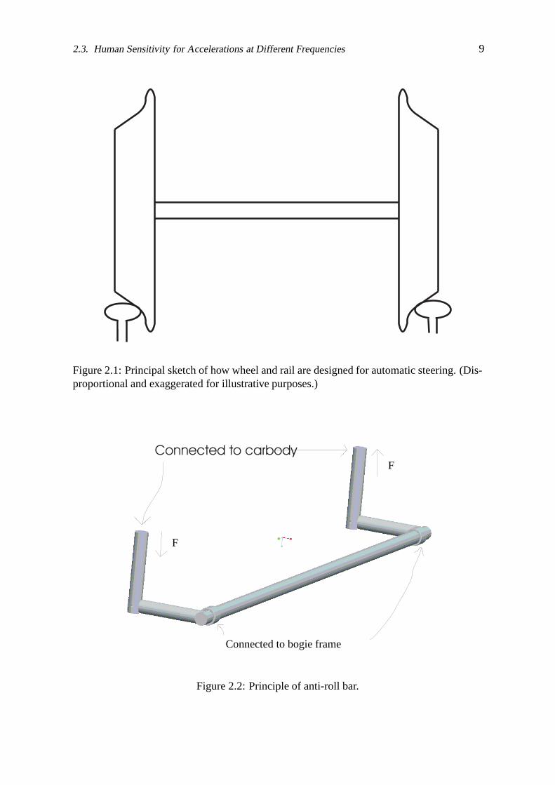
Specific components of the suspension, mentioned in this thesis, are the anti-roll bar, thesecondary vertical dampers, and the air-spring with its pneumatic system. A schematic viewof an anti-roll bar is shown in Figure 2.2. The anti-roll bar counteracts roll between car bodyand bogie frame. This is achieved by the design where the long bar acts as a torsional spring.A difference in deflection between bogie frame and car body, between the two sides wherethe anti-roll bar is attached, will cause a torque in the long bar of the anti-roll bar. Throughthe levers this torque will transfer into forces, F, acting on the car body, which oppose roll.
The secondary vertical dampers’ main task is to dampen roll movement, (Agren 2004–2005), but they will also dampen vertical movement.
The pneumatic system of the air-spring is intended to keep the car body at the same ver-tical position regardless of the amount of payload. This is achieved by adding pressurized airthrough a levelling valve, (Andersson and Berg 1999). The levelling valve can be controlledeither passively, (Andersson and Berg 1999), or actively (Agren 2004–2005).
2.2 Active Suspension in Theory and Practice - Other Research
When the suspension is active, actuators, sensors, and electronic controllers are used, (Goodalland Mei 2006). As a comparison, the conventional, passive, suspension is purely mechani-cal, (Goodall and Mei 2006). There are three major categories of active suspension that arestudied for railway vehicles: active tilting, active secondary suspensions, and active primarysuspensions, (Goodall and Mei 2006).
Tilting of the car body is used to reduce the lateral acceleration experienced by thepassengers in curves, and by this improving passenger comfort, (Goodall and Mei 2006).Active tilting is a standard technology for railway vehicles, (Goodall and Mei 2006).
Secondary active suspension is intended to improve the vehicle dynamic response andprovide a better isolation of the vehicle body to the track irregularities, compared to a fullypassive suspension, (Goodall and Mei 2006). The improved performance could for in-stance be used to improve the comfort for the passengers, (Goodall and Mei 2006). Thefirst commercial use of active secondary suspension was in the Japanese high speed trains(Shinkansen). It was introduced in 2002, and the actuators were installed in the lateral direc-tion, (Goodall and Mei 2006).
Active primary suspension is intended to improve running stability and curving perfor-mance, (Goodall and Mei 2006). There is a trade-off between those issues, and it is difficultto further improve both simultaneously with passive techniques, (Goodall and Mei 2006).When using active primary suspension, the wheelsets can be either independently rotating,or connected by a solid axle, (Goodall and Mei 2006). The idea of active primary suspen-sion is relatively new, but has been successfully tested on a full size roller rig in Germany,(Goodall and Mei 2006).

2.3. Human Sensitivity for Accelerations at Different Frequencies 7
2.3 Human Sensitivity for Accelerations at Different Frequen-cies
Human beings are sensitive to shaking and can find that unpleasant. The amount of discom-fort experienced varies with the frequency of the acceleration. It is possible to weigh theaccelerations for a compound motion together and form a single number, that can be usedto compare the level of discomfort. This number is called ride index or Wertungszahl (Wz).The higher the number is, the worse is the comfort. How to evaluate comfort is described inthis section since one of the criterions on if the secondary suspension is good, is passengercomfort.
2.3.1 Ride index
The ride indexes (Wz-numbers) are calculated using the ISO-standard 2631, (Mechanicalvibration and shock - Evaluation of human exposure to whole-body vibration – Part 1: Gen-eral requirements 1997). This standard contains different weighing curves for calculationof Wz-numbers depending on position of human and direction of vibration. The transferfunctions used to weigh the signals (comfort filters) can be found later in this section. TheWz-number is calculated as follows, (Intec GmbH 2005):
Wz = (100 ·√
σ2w)0.3, (2.1)
where σw is the variance of the output from the comfort filter. The input to the comfort filteris car body accelerations.
Transfer Functions (Comfort Filters)
The transfer functions used to weight the accelerations are
HW,z(s) =(s + 2π · 16)(s2 + 2π·2.5
0.8s + (2π · 2.5)2) · 32.768π
(s2 + 2π·160.63
s + (2π · 16)2)(s2 + 2π·40.8
s + (2π · 4)2)(2.2)
in the vertical direction,
HW,xy(s) =(s + 2π · 4)4π
(s2 + 2π·20.63
s + (2π · 2)2)(2.3)
in the lateral and longitudinal directions, and
Ho(s) =(2π · 100)2
s2 + 2π·1000.71
s + (2π · 100)2(2.4)
and
Hu(s) =s2
s2 + 2π·0.40.71
s + (2π · 0.4)2(2.5)
for all directions, (Intec GmbH 2005).
8 2. Background Theory
The total transfer function of the comfort filter is calculated by HC,i(s) = HW,i(s) ·Hu(s) · Ho(s), where HW,i(s) is the weighting filter, and Hu(s) and Ho(s) together makesup the band limiting filter, (Intec GmbH 2005). The subscript i could be either xy or z.When the subscript is xy, the filter is valid in the lateral and longitudinal directions of thevehicle when the passengers are seated or standing. When the subscript is z, the filter isvalid in the vertical direction of the vehicle when the passengers are seated or standing. Themagnitudes of the total transfer functions, in the frequency interval 0.1–100 Hz, are plottedin Figure 2.3 and Figure 2.4. The accelerations are causing most discomfort in the frequencyinterval where the magnitude of the comfort filters are largest.
Crest Factors
To check whether it is correct in a specific case to calculate the comfort values using Wz-numbers, the crest factors are studied. The crest factor is defined as the quotient betweenthe maximum acceleration and the rms-value of the acceleration, amax/arms. When the max-imum and rms-value are determined on the weighted signal, the crest factor should be nohigher than 9. If the crest factor is higher than 9, the effect of the motion may be underes-timated. Otherwise it is normally sufficiently accurate. The calculation and interpretationof the crest factor are described in the ISO-standard 2631-1:1997(E), (Mechanical vibra-tion and shock - Evaluation of human exposure to whole-body vibration – Part 1: Generalrequirements 1997).
Motion Sickness
There is also a weighting curve in the vertical direction for motion sickness (not shownhere). This has it peak just below 0.2 Hz, (Andersson et al. 2004). It will however be seen inChapter 6, that this is outside the range of the validity of the linear model used in this thesis.The motion sickness aspect has therefore not been considered in this thesis.
2.3. Human Sensitivity for Accelerations at Different Frequencies 9
Figure 2.1: Principal sketch of how wheel and rail are designed for automatic steering. (Dis-proportional and exaggerated for illustrative purposes.)
Connected to carbody
Connected to bogie frame
F
F
Figure 2.2: Principle of anti-roll bar.

10 2. Background Theory
10−1
100
101
102
−40
−35
−30
−25
−20
−15
−10
−5
0
5
Mag
nitu
de[d
B]
Frequency [Hz]
Figure 2.3: Magnitude of total transfer function of the comfort filter, HC,z(s).

2.3. Human Sensitivity for Accelerations at Different Frequencies 11
10−1
100
101
102
−40
−35
−30
−25
−20
−15
−10
−5
0
5
Mag
nitu
de[d
B]
Frequency [Hz]
Figure 2.4: Magnitude of total transfer function of the comfort filter, HC,xy(s).


chapter iii
research objective, methodology andthesis structure
In this chapter the research objectives are stated, an overview on how the work has beencarried out is presented, and it is described how the different chapters connect to each other.
3.1 Research Objective
The long term goal is to replace passive suspension components with active, while at thesame time improving vehicle performance. Replacing some passive suspension componentswith active could reduce the weight and cost of the vehicle, (Agren 2004–2005). Addingactive suspension may also improve passenger comfort without increasing the deflectionswithin the suspension, or, similarly, allow the vehicle to be run at higher speeds or on lesssmooth tracks, with comfort and deflection kept at today’s levels, (Goodall and Mei 2006).
The active suspension design can be divided into four areas: which passive componentsthat are replaced with active, where the active components are placed, which control strategythat is used, and which active components, such as sensors and actuators, that are used. In thisthesis, only control strategy is considered. Other factors are decided without investigatingother options. The sensors and actuators are assumed to be ideal, which means that they haveno dynamics in themselves, and are without error or noise.
In this thesis, there is no intention to actually remove any components. It is assumed, thatthe forces exerted by the passive components, can be calculated approximately and added tothe control law, once a control law has been found.
The research objective in this thesis is to analyze a model of a railway vehicle, and todo background studies to prepare for the developing of a control law to be used in an activesuspension. The active suspension should be fitted in the vertical direction, between thebogie frames and the car body.
3.1.1 Evaluation Criteria
The main criterion has been chosen as passenger comfort. Passenger comfort is decided bythe accelerations, in a way which is described in detail in Section 2.3. Improving comforttends to increase (worsen) the deflection, which also must be kept under control. Therefore,also deflection is an evaluation criterion. More specifically, the choice has fallen on studyingthe maximum deflection, since the space available is critical. Also, the requirement on force,power, and speed of the actuator needs to be kept an eye on.

14 3. Research Objective, Methodology and Thesis Structure
3.2 General Methods
The work has been purely theoretical. The focus has been on computer simulations andanalysis. For simulation purposes a large, non-linear model has been used. For analysis anddesign, linear, and for some cases reduced, models have been used. Those have all beenderived from the large, non-linear model.
3.2.1 Software Tools
The model is modeled in the software Simpack, which is a multibody simulation tool, fromINTEC GmbH, Weßling, Germany. Simpack is used with the module Simpack Rail, whichsupports railway simulations. Also, linear state matrices are exported from Simpack to Mat-lab. In Matlab analysis and control design are carried out. Matlab is used with Control Sys-tems Toolbox and Simulink, also from MathWorks, and with Slicot. Slicot is a subroutine li-brary based on BLAS and LAPACK routines and further developed, partly in the frameworkof the European project NICONET1, (Benner, Mehrmann, Sima, Huffel and Varga 1998).Simulations are carried out in Simpack, using the solver SODASRT, and in Simulink, usingODE45 (Dormand-Prince).
3.2.2 Linearization
In the software Simpack, there is a build-in support to create and export linear models. Avelocity is set, inputs and outputs are chosen, the wheel-rail contact is linearized, the vehicleis put at (or as close as possible to) equilibrium. Then a linear state space model is createdand exported in a format that can be read by Matlab.
During the linearization, the vehicle is positioned on a straight, flat (not leaning) trackwithout any disturbances, and is running at approximately 1 km/h. This velocity is set be-cause zero velocity cannot be used with tangential forces (Intec GmbH 2003). Also, a marginis kept to high velocities, which could induce instability and worsen numerical issues.
3.3 Work Flow and Thesis Structure
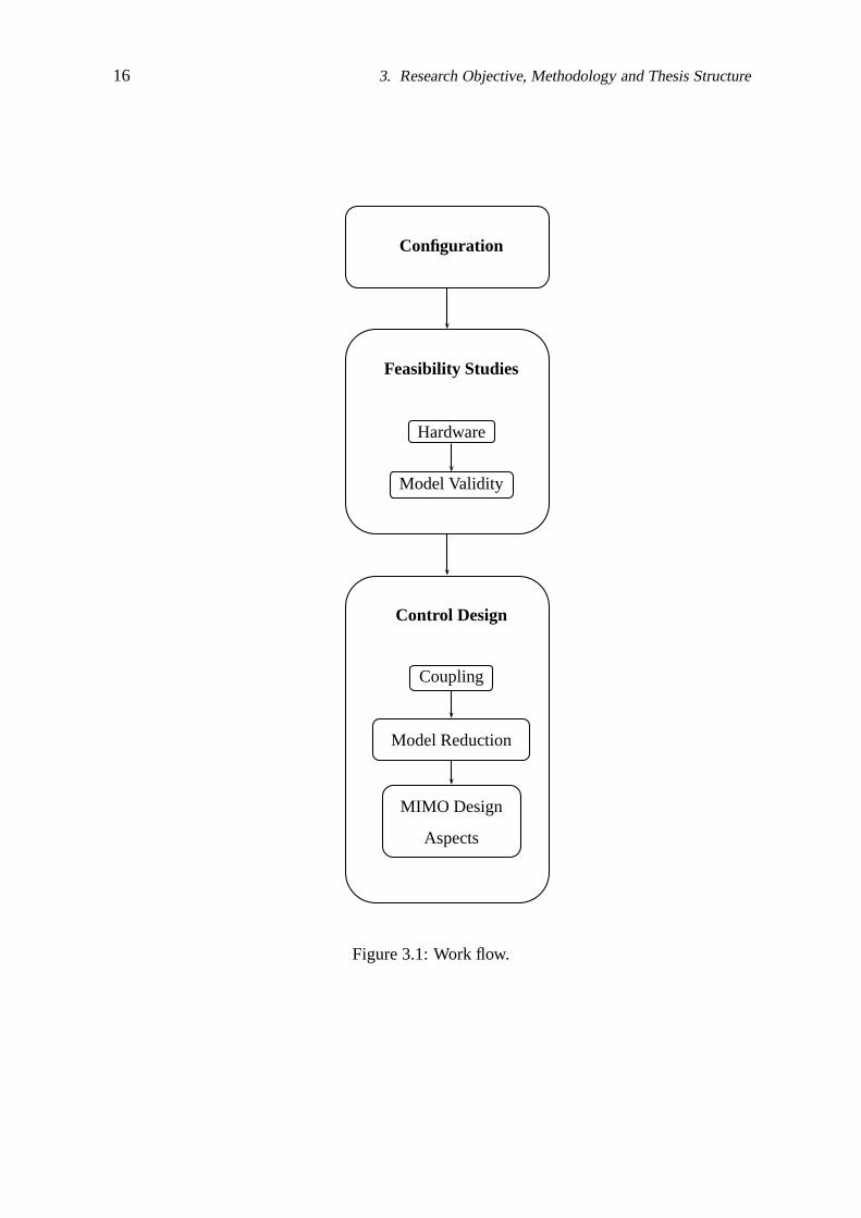
In this section, the work flow is described, together with references to in which chapter eachpart of the work can be found. An overview of the work flow can be seen in Figure 3.1. Amore detailed description, that refers to that figure, follows below.
The first main box in Figure 3.1 is labeled ”Configuration”. The more general config-urations, regarding choices of model parameters and where the active suspensions is fitted,are described in Chapter 4. In the same chapter the vehicle is briefly described. Also, themeasured disturbances are plotted and analyzed. More specific choices of running scenarioare described in respective chapter, most notably in Chapter 5.
The second main box in Figure 3.1 is labeled ”Feasibility Studies”. Here it is investi-gated whether or not it is reasonable to go on with finding a control strategy. In this box,the first box is labeled ”Hardware”. This is referring to the work in Chapter 5, where itis estimated what is required by the actuators in an active secondary suspension, if fitted
1http://www.icm.tu-bs.de/NICONET/

3.3. Work Flow and Thesis Structure 15
as desired. The purpose is to estimate if it is feasible to implement physically, and in thatway make the basis of the decision to move on with trying to find a control strategy for thisconfiguration. The second box is labeled ”Model Validity”. This is referring to the workin Chapter 6, where the validity of the linear model is estimated, in order to check that themodel can be used in the frequency region that is important from a comfort point of view.
The third main box in Figure 3.1 is labeled ”Control Design”. This term is used herefor some background work aiming towards finding a control. (The actual design is leftas future work.) In this box, the first box is labeled ”Coupling”. This is referring to thework in Chapter 7, of which the purpose is to investigate the possibilities of splitting theproblem into several problems with one input and one output each (SISO design). Herethe coupling between different inputs and outputs are studied, and attempts are made atdecoupling. This fails. The second box is labeled ”Model Reduction”. This is referring tothe work in Chapter 8. Since the attempts at SISO design were unsuccessful, it is desired totry design a control system for using all input and outputs at once (MIMO design). However,to make that task more reasonable, the system needs to be simplified (reduced). The last boxis labeled ”MIMO Design Aspects”. Here some issues with MIMO design, concentrating onlinear quadratic (LQ) design, are explored.
16 3. Research Objective, Methodology and Thesis Structure
Configuration
Feasibility Studies
Hardware
Model Validity
Control Design
Coupling
Model Reduction
MIMO Design
Aspects
Figure 3.1: Work flow.

chapter iv
model
4.1 Model Structure
All vehicle models used in this report are based on the same three-dimensional, non-linearmodel of a railway vehicle, obtained from Bombardier Transportation, modeled by BjornRoos. That model is modeled in an MBS (Multi Body Systems) program, and is describedin this chapter.
4.1.1 Vehicle
The vehicle is a passenger vehicle. However, where nothing else is noted in this thesis, thepassengers are not included in the model. Without passengers the model has 330 states.In some cases passengers are modeled. This is described in Appendix A. The maximumallowed velocity for the vehicle is 200 km/h.
The railway vehicle consists of a single car. It is modeled using rigid bodies, whichare connected with various joints and force elements. The car is not quite symmetric in anydirection.
4.1.2 Active Suspension
The active suspension (force inputs) has been positioned in the secondary suspension in thevertical direction. The secondary suspension is the suspension between the car body and thebogie frame, as shown in Figure 4.1. To be able to handel both vertical and roll disturbances,there has to be control inputs on both sides of the vehicle.
Four actuators are used. The actuators are placed in the same spots as the vertical sec-ondary dampers. This is not a problem in simulations, and won’t be in reality either, sinceit’s assumed that the secondary dampers will be removed before any physical implementationwill be attempted.
4.1.3 Inputs and Outputs
The control inputs are actuator forces.The outputs are car body acceleration as well as the distances between car body and
bogie frames. The disturbance inputs have their origin in rail imperfections, which are de-scribed as deviations in lateral, vertical, and roll directions. For the simulations (not linearanalyzes), there are also deviations in gauge (distance between the rails).
18 4. Model
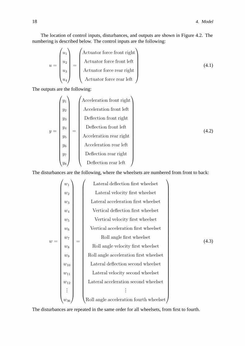
The location of control inputs, disturbances, and outputs are shown in Figure 4.2. Thenumbering is described below. The control inputs are the following:
u =
⎛⎜⎜⎜⎜⎜⎜⎝
u1
u2
u3
u4
⎞⎟⎟⎟⎟⎟⎟⎠
=
⎛⎜⎜⎜⎜⎜⎜⎝
Actuator force front right
Actuator force front left
Actuator force rear right
Actuator force rear left
⎞⎟⎟⎟⎟⎟⎟⎠
(4.1)
The outputs are the following:
y =
⎛⎜⎜⎜⎜⎜⎜⎜⎜⎜⎜⎜⎜⎜⎜⎜⎜⎜⎜⎝
y1
y2
y3
y4
y5
y6
y7
y8
⎞⎟⎟⎟⎟⎟⎟⎟⎟⎟⎟⎟⎟⎟⎟⎟⎟⎟⎟⎠
=
⎛⎜⎜⎜⎜⎜⎜⎜⎜⎜⎜⎜⎜⎜⎜⎜⎜⎜⎜⎝
Acceleration front right
Acceleration front left
Deflection front right
Deflection front left
Acceleration rear right
Acceleration rear left
Deflection rear right
Deflection rear left
⎞⎟⎟⎟⎟⎟⎟⎟⎟⎟⎟⎟⎟⎟⎟⎟⎟⎟⎟⎠
(4.2)
The disturbances are the following, where the wheelsets are numbered from front to back:
w =
⎛⎜⎜⎜⎜⎜⎜⎜⎜⎜⎜⎜⎜⎜⎜⎜⎜⎜⎜⎜⎜⎜⎜⎜⎜⎜⎜⎜⎜⎜⎜⎜⎜⎜⎜⎜⎜⎝
w1
w2
w3
w4
w5
w6
w7
w8
w9
w10
w11
w12
...
w36
⎞⎟⎟⎟⎟⎟⎟⎟⎟⎟⎟⎟⎟⎟⎟⎟⎟⎟⎟⎟⎟⎟⎟⎟⎟⎟⎟⎟⎟⎟⎟⎟⎟⎟⎟⎟⎟⎠
=
⎛⎜⎜⎜⎜⎜⎜⎜⎜⎜⎜⎜⎜⎜⎜⎜⎜⎜⎜⎜⎜⎜⎜⎜⎜⎜⎜⎜⎜⎜⎜⎜⎜⎜⎜⎜⎜⎝
Lateral deflection first wheelset
Lateral velocity first wheelset
Lateral acceleration first wheelset
Vertical deflection first wheelset
Vertical velocity first wheelset
Vertical acceleration first wheelset
Roll angle first wheelset
Roll angle velocity first wheelset
Roll angle acceleration first wheelset
Lateral deflection second wheelset
Lateral velocity second wheelset
Lateral acceleration second wheelset...
Roll angle acceleration fourth wheelset
⎞⎟⎟⎟⎟⎟⎟⎟⎟⎟⎟⎟⎟⎟⎟⎟⎟⎟⎟⎟⎟⎟⎟⎟⎟⎟⎟⎟⎟⎟⎟⎟⎟⎟⎟⎟⎟⎠
(4.3)
The disturbances are repeated in the same order for all wheelsets, from first to fourth.

4.2. Measured Input Data 19
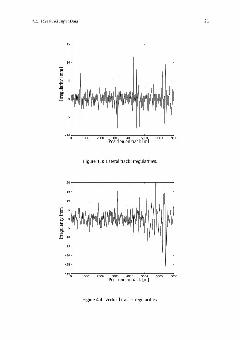
4.2 Measured Input Data
This section deals with the track irregularities exciting the vehicle. The irregularities havebeen obtained from Bombardier Transportation, and have been measured with 0.5 m interval.That means that if, for example, disturbances up to 20 Hz are desired, the vehicle needs tobe run at at least 72 km/h. (The model itself is valid also at lower velocities, but would needother inputs to enable evaluation of the entire interesting frequency region.)
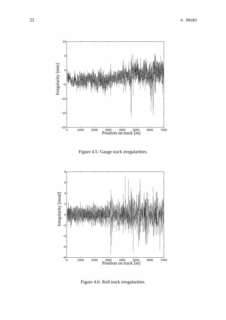
4.2.1 Track Irregularities in Spatial Domain
The measured track irregularities used in this report are shown in Figure 4.3 – Figure 4.6.Note that the scale on the y-axis is not the same in all figures.
4.2.2 Track Irregularities in Frequency Domain
Figure 4.7 – Figure 4.10 show the spatial frequency content of the track irregularities. Thefrequency content in the time domain depends on vehicle velocity. The dependency of thevelocity is due to the fact that when the spatial irregularities are traversed faster or slower,the vehicle will, for the same spatial irregularities, feel different frequencies in Hz. Note thatthe scale on the y-axis is not the same in all figures.
The frequency content is calculated, using the Welch’s method for power spectral densityestimate, with a Hamming window, 8 sections, and 50% overlap. Welch’s method is chosen,because the PSD is very noise if calculated directly, and Welch’s method smoothes this outa bit.
The data is, as previously mentioned, sampled at 0.5 meters interval. The peaks in theirregularities at approximately 0.32 m−1 (in Figure 4.7 – Figure 4.10) could be due to an aliasphenomenon from the sleeper passage, which in itself has a too high frequency to renderproperly with those measurement data. The sleeper distance is usually 0.60–0.65 metersat the main railway lines in Sweden, (Andersson and Berg 1999). This corresponds to aspatial frequency of 1.54–1.67 m−1. With the sampling frequency 2 m−1, this shows up as0.33–0.46 m−1. (A sleeper distance of 0.595 m would look like 0.32 m−1)

20 4. Model
Secondary suspension
Bogie frame
Car body
Figure 4.1: Schematic picture of where the secondary suspension is located. (It is within thedotted box.)
−10 −5 0 5 10−6
−4
−2
0
2
4
6
Car bodyOutput accelerationOutput deflectionInput controlInput disturbance
[m]
[m]
Figure 4.2: Location of inputs and outputs, top view.
4.2. Measured Input Data 21
0 1000 2000 3000 4000 5000 6000 7000−10
−5
0
5
10
15
Irre
gula
rity
[mm
]
Position on track [m]
Figure 4.3: Lateral track irregularities.
0 1000 2000 3000 4000 5000 6000 7000−30
−25
−20
−15
−10
−5
0
5
10
15
20
Irre
gula
rity
[mm
]
Position on track [m]
Figure 4.4: Vertical track irregularities.
22 4. Model
0 1000 2000 3000 4000 5000 6000 7000−20
−15
−10
−5
0
5
10
Irre
gula
rity
[mm
]
Position on track [m]
Figure 4.5: Gauge track irregularities.
0 1000 2000 3000 4000 5000 6000 7000−8
−6
−4
−2
0
2
4
6
8
Irre
gula
rity
[mra
d]
Position on track [m]
Figure 4.6: Roll track irregularities.

4.2. Measured Input Data 23
10−2
10−1
100
10−12
10−11
10−10
10−9
10−8
10−7
10−6
10−5
Pow
er/f
requ
ency
[m2/m
−1]
Spatial frequency [m−1]
Figure 4.7: Frequency content of lateral track irregularities, by Welch power spectral densityestimate.
10−2
10−1
100
10−11
10−10
10−9
10−8
10−7
10−6
10−5
10−4
Pow
er/f
requ
ency
[m2/m
−1]
Spatial frequency [m−1]
Figure 4.8: Frequency content of vertical track irregularities, by Welch power spectral den-sity estimate.

24 4. Model
10−2
10−1
100
10−11
10−10
10−9
10−8
10−7
10−6
10−5
10−4
Pow
er/f
requ
ency
[m2/m
−1]
Spatial frequency [m−1]
Figure 4.9: Frequency content of gauge track irregularities, by Welch power spectral densityestimate.
10−2
10−1
100
10−12
10−11
10−10
10−9
10−8
10−7
10−6
10−5
Pow
er/f
requ
ency
[rad
2/m
−1]
Spatial frequency [m−1]
Figure 4.10: Frequency content of roll track irregularities, by Welch power spectral densityestimate.

chapter v
feasibility considerations
The purpose of this chapter is to investigate if it seems reasonable to use active suspensionto replace some of the passive components. This is from the point of view if it is reasonableto assume that it is possible to construct actuators that are able to deal with the task of activesecondary vertical suspension. More specifically, the purpose of this chapter is to decidewhether it is reasonable to switch to one of the active designs described in Section 5.2.1.
For this purpose, requirements on forces that need to be delivered by an active secondaryrailway suspension system are investigated, as well as the active system’s estimated powerconsumption. This is done by calculating the corresponding properties for a specific passen-ger train with passive suspension system from Bombardier Transportation, for the differentscenarios. Although the future choice of control strategy will affect the requested forces andeffective powers from the actuators, and thus the requirements on actuator performance, thepassive behavior is used as an approximation of what is required.
Both quasi-static and dynamic conditions are studied. Through this quasi-static forces,dynamic forces, and powers, that need to be delivered by an actuator, are obtained.
5.1 Background Theory
This section describes the theoretical background that choices and conclusions in this chapterare based on.
5.1.1 Railway Vehicle
Speed Limitations
If the vehicle is run through a curve, the maximum allowed velocity, vmax, is limited also bythe maximum allowed lateral acceleration, ay,max by the following equation:
vmax =
√R(ay,max + g
ht
2bo
), (5.1)
where R is the curve radius, g is the acceleration of gravity, ht is the cant (distance that theouter rail is raised in a curve), and 2bo is the distance between the nominal wheel-rail contactpoints on the left and right rail, (Andersson et al. 2004). The maximum allowed lateral(track plane) acceleration is 0.98 m/s2 for vehicles of category B is Sweden, (Anderssonet al. 2004). This is the category the vehicle studied in this thesis belongs to.
26 5. Feasibility Considerations
Friction
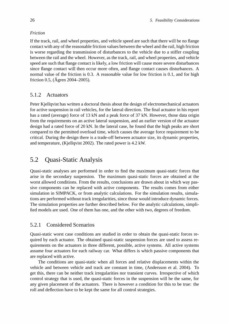
If the track, rail, and wheel properties, and vehicle speed are such that there will be no flangecontact with any of the reasonable friction values between the wheel and the rail, high frictionis worse regarding the transmission of disturbances to the vehicle due to a stiffer couplingbetween the rail and the wheel. However, as the track, rail, and wheel properties, and vehiclespeed are such that flange contact is likely, a low friction will cause more severe disturbancessince flange contact will then occur more often, and flange contact causes disturbances. Anormal value of the friction is 0.3. A reasonable value for low friction is 0.1, and for highfriction 0.5, (Agren 2004–2005).
5.1.2 Actuators
Peter Kjellqvist has written a doctoral thesis about the design of electromechanical actuatorsfor active suspension in rail vehicles, for the lateral direction. The final actuator in his reporthas a rated (average) force of 13 kN and a peak force of 37 kN. However, those data originfrom the requirements on an active lateral suspension, and an earlier version of the actuatordesign had a rated force of 20 kN. In the lateral case, he found that the high peaks are shortcompared to the permitted overload time, which causes the average force requirement to becritical. During the design there is a trade-off between actuator size, its dynamic properties,and temperature, (Kjellqvist 2002). The rated power is 4.2 kW.
5.2 Quasi-Static Analysis
Quasi-static analyses are performed in order to find the maximum quasi-static forces thatarise in the secondary suspension. The maximum quasi-static forces are obtained at theworst allowed conditions. From the results, conclusions are drawn about in which way pas-sive components can be replaced with active components. The results comes from eithersimulation in SIMPACK, or from analytic calculations. For the simulation results, simula-tions are performed without track irregularities, since those would introduce dynamic forces.The simulation properties are further described below. For the analytic calculations, simpli-fied models are used. One of them has one, and the other with two, degrees of freedom.
5.2.1 Considered Scenarios
Quasi-static worst case conditions are studied in order to obtain the quasi-static forces re-quired by each actuator. The obtained quasi-static suspension forces are used to assess re-quirements on the actuators in three different, possible, active systems. All active systemsassume four actuators for each railway car. What differs is which passive components thatare replaced with active.
The conditions are quasi-static when all forces and relative displacements within thevehicle and between vehicle and track are constant in time, (Andersson et al. 2004). Toget this, there can be neither track irregularities nor transient curves. Irrespective of whichcontrol strategy that is used, the quasi-static forces in the suspension will be the same, forany given placement of the actuators. There is however a condition for this to be true: theroll and deflection have to be kept the same for all control strategies.

5.2. Quasi-Static Analysis 27
For the quasi-static forces, three different scenarios where currently used componentswill be replaced with active, are studied. Those are
Scenario 1. Remove anti-roll bar and secondary vertical damper. (Studied in infinitecurve.) This scenario is studied by passive simulations in Section 5.2.2, andby analytic calculations in Section 5.2.3. The models for the analytic calcu-lations are more simplified than those for the simulations. Another differenceis that the analytical calculations deals with a tougher condition on the quasi-static roll performance, namely that the car body should be kept parallel tothe bogie. The passive simulations will give the quasi-static forces needed tokeep the same quasi-static roll performance as of the current passive vehicle,which does not require the car body to be quite parallel to the bogie.
Scenario 2. Remove pneumatic system of the air-spring (not the air-spring itself). (Stud-ied for payload deviations.) This scenario is studied in Section 5.2.4.
Scenario 3. Combine the two scenarios above. This scenario is studied in Section 5.2.5.
The quasi-static forces are studied since the force that an actuator can deliver during along period of time is lower than the peak force it can deliver, and specifications need thusto be stated for quasi-static forces. The limit for quasi-static forces is lower than the limitfor peak forces, since temperature is a limiting factor in actuator design, (Kjellqvist 2002).The temperature will not reach its maximum value for a given force instantly. Also, thequasi-static forces can be decided exactly when the running conditions and performance re-quirements are known, which makes it easy to find a requirement for quasi-static conditions.
5.2.2 Force to Control Roll, Passive Simulations (Scenario 1)
In the passive case, the quasi-static forces that are controlling the roll, are exerted by theanti-roll bars and the air-springs. The maximum quasi-static forces on the anti-roll bar areobtained in the worst allowed curves at maximum vehicle load. The worst possible casewould be, when the lateral (track plane) acceleration is at its maximum allowed value.
A simple way to imitate the worst case curve, is to do a simulation using a straight track,with a fictitious component of gravity pointing in the lateral direction. Such simulations arerun until initial transients decay and the forces are stabilized.
Simulation data are as follows:
• Mass AW3 (100 seated passengers in the car and 2 standing passengers per squaremeter. Carbody and passengers weighs 53052 kg together, where the payload part is10776 kg. Each person weighs 80 kg.) (Roos 2005).
• Vehicle velocity 0.1 m/s. (The velocity needs to be greater than zero for simulationpurposes, (Intec GmbH 2003).)
• Simulation time is 40 s, which suffices to let the transients decay.
• Pre-loaded forces (nominal forces) of the model’s preloaded force elements are calcu-lated analytically outside of SIMPACK, to get static equilibrium at straight track withno cant deficiency or cant excess. These are not consistent with the fictitious skewedgravity vector, which implies that the vehicle is not initially at equilibrium.

28 5. Feasibility Considerations
• Fictitious gravity vector:eithergx = 0 m/s2, gy = 0.98 m/s2, gz = 9.76 m/s2, corresponding to the case when theentire lateral part of the gravity comes from the true acceleration of gravity. Here theresultant gravity is 9.81 m/s2.orgx = 0 m/s2, gy = 0.98 m/s2, gz = 9.81 m/s2, corresponding to the case when no partof the lateral part of the gravity comes from the true acceleration of gravity, but comesfrom the centripetal force instead. Here, the resultant fictitious gravity is 9.86 m/s2.
The simulation results yield that the resulting force in each anti-roll bar is 32.3 kN, forboth cases of fictitious gravity vector. Also, each air-spring contributes to limit the roll.However, since there is no intention to remove the air-springs here (see Section 3.1), thiscontribution is assumed to remain also for a modified system, and is therefore not consideredhere.
5.2.3 Force to Control Roll, Carbody Parallel with Bogie (Scenario 1)
As opposed to the previous section, this section does not deal with the passive system. In-stead, an active system is studied. Here, the assumption is made that quasi-statically, thecar body should be kept parallel to the bogie. That is a requirement for better performanceregarding roll than in the passive case. If the roll is to be compensated in a way that keepsthe car body parallel to the bogie, higher forces than what is required to imitate the passivesystem will be needed. See the calculations below. For the following calculations, regard-ing components, it is assumed that the air-springs are kept at their current positions in thesuspension design, but the anti-roll bar and secondary dampers have been removed from theoriginal model. Instead, actuators are introduced at the former position of the dampers.
In Figure 5.1, all variables that are not explicitly defined in this section, are defined. αis the angle between the bogie frame and the wheelset. This angle is assumed to be small.θ is defined in Equation 5.12 – Equation 5.14. COG means center of gravity. gtot is thetotal acceleration caused by the combination of the maximum allowed lateral acceleration,a = 0.98 m/s2, see Section 5.2.2, and the acceleration of gravity, g = 9.81 m/s2. The lateralacceleration, a, could origin from either a centripetal force, or, if the track has a cant, theacceleration of gravity. It could also be a combination of both. The remaining part of theacceleration of gravity, that is pointing in the vertical direction, is called gz. The Pythagoreantheorem yields
gtot =√
g2z + a2. (5.2)
Force equilibrium in the vertical direction, with positive direction upwards, gives for the carbody
Fsl + Fal + Far + Fsr − mgtot cos θ = 0. (5.3)
Since the car body is kept parallel to the bogie, the displacements of the left and right air-spring are the same, and thus their forces are the same. In order to minimize the need ofactive force, the air-springs should carry the load of the car body. Thus
Fsl = Fsr =mgtot
2cos θ (5.4)

5.2. Quasi-Static Analysis 29
and
Fal + Far = 0. (5.5)
Moment equilibrium clockwise around the connection point of the left actuator to the carbody yields
Fsl(d − e) + emgtot cos θ + hmgtot sin θ − 2Fare − Fsr(d + e) = 0. (5.6)
Using Equation 5.4 and Equation 5.6, and solving for Far yields
Far =mgtoth
2esin θ. (5.7)
The force required by an actuator is increased with increased car body mass, increased totalacceleration acting on the car body, increased distance to the center of gravity of the car body,and increased angle between the resultant force from the accelerations and the bogie. Theforce needed is decreased with increased distances from the lateral center of the car bodyand the connection points of the actuators.
To find out the additional angle, α, caused by the deflections in the primary suspensions,equilibrium for the primary suspension was set up, see Equation 5.8 – Equation 5.12.
Fpl + Fpr − Fsl − Fal − Far − Fsr = 0, (5.8)
Fsl(f − d) + Fal(f − e) + Far(f + e) + Fsr(f + d) − Fpr2f = 0 (5.9)
xl =Fpl
kp
(5.10)
xr =Fpr
kp(5.11)
α = arctanxr − xl
2f(5.12)
kp is the vertical spring value of the primary suspension, and the other variables are definedin Figure 5.1. The angle α is then added to the angle from the track plane acceleration, θ0.Thus
θ = θ0 + α, (5.13)
where
θ0 = arcsina
gz, (5.14)
where a is the maximum allowed lateral acceleration, 0.98 m/s2, see Section 5.2.2, and gz isthe vertical part of the acceleration of gravity. gz can vary between 9.76 m/s2 and 9.81 m/s2,depending on how much from the gravity that will be a part of a. The calculations wereiterated until the angles and forces did not change anymore. The resulting force in eachactuator is 39.3 kN, for all allowed values of gz, at maximum payload. This can be comparedwith the result from Section 5.2.2, which was that the quasi-static force needed from eachactuator is 32.3 kN. Thus a higher quasi-static force is needed to keep the car body parallelto the bogie, than for keeping the roll at the level of today’s passive suspension.
30 5. Feasibility Considerations
5.2.4 Air-Spring Deviation from Equilibrium (Scenario 2)
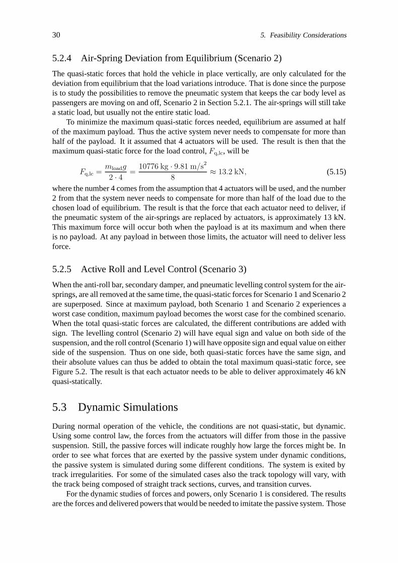
The quasi-static forces that hold the vehicle in place vertically, are only calculated for thedeviation from equilibrium that the load variations introduce. That is done since the purposeis to study the possibilities to remove the pneumatic system that keeps the car body level aspassengers are moving on and off, Scenario 2 in Section 5.2.1. The air-springs will still takea static load, but usually not the entire static load.
To minimize the maximum quasi-static forces needed, equilibrium are assumed at halfof the maximum payload. Thus the active system never needs to compensate for more thanhalf of the payload. It it assumed that 4 actuators will be used. The result is then that themaximum quasi-static force for the load control, Fq,lc, will be
Fq,lc =mloadg
2 · 4 =10776 kg · 9.81 m/s2
8≈ 13.2 kN, (5.15)
where the number 4 comes from the assumption that 4 actuators will be used, and the number2 from that the system never needs to compensate for more than half of the load due to thechosen load of equilibrium. The result is that the force that each actuator need to deliver, ifthe pneumatic system of the air-springs are replaced by actuators, is approximately 13 kN.This maximum force will occur both when the payload is at its maximum and when thereis no payload. At any payload in between those limits, the actuator will need to deliver lessforce.
5.2.5 Active Roll and Level Control (Scenario 3)
When the anti-roll bar, secondary damper, and pneumatic levelling control system for the air-springs, are all removed at the same time, the quasi-static forces for Scenario 1 and Scenario 2are superposed. Since at maximum payload, both Scenario 1 and Scenario 2 experiences aworst case condition, maximum payload becomes the worst case for the combined scenario.When the total quasi-static forces are calculated, the different contributions are added withsign. The levelling control (Scenario 2) will have equal sign and value on both side of thesuspension, and the roll control (Scenario 1) will have opposite sign and equal value on eitherside of the suspension. Thus on one side, both quasi-static forces have the same sign, andtheir absolute values can thus be added to obtain the total maximum quasi-static force, seeFigure 5.2. The result is that each actuator needs to be able to deliver approximately 46 kNquasi-statically.
5.3 Dynamic Simulations
During normal operation of the vehicle, the conditions are not quasi-static, but dynamic.Using some control law, the forces from the actuators will differ from those in the passivesuspension. Still, the passive forces will indicate roughly how large the forces might be. Inorder to see what forces that are exerted by the passive system under dynamic conditions,the passive system is simulated during some different conditions. The system is exited bytrack irregularities. For some of the simulated cases also the track topology will vary, withthe track being composed of straight track sections, curves, and transition curves.
For the dynamic studies of forces and powers, only Scenario 1 is considered. The resultsare the forces and delivered powers that would be needed to imitate the passive system. Those

5.3. Dynamic Simulations 31
indicate roughly what will be required from an active system. The reason that the results arenot exact is, as mentioned above, that the forces and powers will depend on control strategy.
The dynamic studies also yield the vehicle performance in the passive system, concern-ing deflections, roll, and comfort. These results can be used as requirements for an activesystem.
5.3.1 Simulated Cases
To obtain the dynamic forces in the secondary suspension, simulations are run at some certaincircumstances according to the list below. Some circumstances are chosen to be normal,other to be as bad as possible. Some parameters for the simulation that might need furtherexplanation are explained here:
• VelocityFor all cases listed below, the velocity is the maximum allowed for the vehicle, con-sidering the curve radius.
• Track irregularitiesFor all cases, measured track irregularities are used. In some cases, the amplitude ofthe irregularities are multiplied with some factor. Then the irregularities will corre-spond to a track with larger irregularities, since the factors are greater than 1.
• FrictionWhere the friction is not chosen as normal friction, the friction is chosen to causemaximum disturbance. In curves the friction are chosen to maximize the risk of flangecontact.
The following cases were evaluated:Case 1 (straight track)
• Straight track.
• Velocity 200 km/h.
• No payload – this will give the worst comfort, since then the quotient between theunsprung and sprung mass reaches its highest value.
• Measured track irregularities multiplied with 1.5.
• Friction 0.5 (high friction).
Case 2 (tight curve)
• Curve radius 300 m.
• Cant 150 mm.
• Velocity 87 km/h.
• No payload.
• Measured track irregularities multiplied by 2.

32 5. Feasibility Considerations
• Friction 0.1 (low friction).
Case 3 (tight curve, same as case 2 but with full payload)
• Curve radius 300 m.
• Cant 150 mm.
• Velocity 87 km/h (maximum to stay within allowed lateral acceleration (Anderssonand Berg 1999)).
• Full payload.
• Measured track irregularities multiplied by 2.
• Friction 0.1 (low friction).
Case 4 (measured track)
• Measured track.
• Velocity 200 km/h.
• No payload.
• Measured track irregularities.
• Friction 0.3 (normal friction).
Case 5 (measured track, same as case 4 but with full payload)
• Measured track.
• Velocity 200 km/h.
• Full payload.
• Measured track irregularities.
• Friction 0.3 (normal friction).
5.3.2 Simulation Results
This section describes the simulation results. The forces and powers can be used to estimatewhat will be required by the actuators if active suspension is used.
Simulations are run for the 5 different conditions described in Section 5.3.1. In thefollowing sub-sections, maximum and minimum values come from varying force elementsand simulation conditions. For a complete list of results, see Appendix D.
Forces in Anti-Roll Bar and Damper
The maximum peak force in the anti-roll bar is 41 kN. This occurs in case 3 (curve with fullload). The maximum mean of the absolute value of the force in the anti-roll bar is 32.0 kN.This also occurs in case 3.
The maximum peak force in the vertical damper in the secondary suspension is smaller,6.1 kN. This occurs in case 1 (straight track).

5.4. Concluding Remarks 33
Ideal Power Dissipation or Consumption in Anti-Roll Bar and Damper
The power dissipation in the secondary damper is, naturally, modelled as force times velocity(P = F ·v, (Nordling and Osterman 1996)). This yields a maximum peak power of 1.9 kW,which occurs in case 1.
The power that corresponds to the anti-roll bar is calculated in a less intuitive way. Theforce in the anti-roll bar is (for each component x, y, and z) multiplied with the velocitybetween the connection between the anti-roll bar and the car body, and a point on the bogiethat is originally right below the connection point. The reason of this choice is that this yieldsthe power needed if the anti-roll bar is replaced by an actuator placed in that position. Themaximum absolute value of the power derived from the anti-roll bar is 4.4 kW, also this isoccurring in case 1.
The differences in powers in the anti-roll bars and dampers are larger than the differencesin forces in the anti-roll bars and dampers. This indicates that the velocity is low near themaximum deflection. That is as expected, since that is where the movement change direction.
5.4 Concluding Remarks
First, the quasi-static conditions are discussed:For Scenario 1, the active suspension replaces the anti-roll bar and the secondary vertical
damper. Then the results show that each actuator must be able to deliver quasi-static forcesof roughly 32 kN.
For Scenario 2, the pneumatic pump system for the air-springs, which adapts the airpressure to compensate for payload variations, is removed. Instead, the active suspensionwill be used to keep the car body at the same vertical position regardless of the amount ofpayload. This requires a quasi-static force from each actuator of about 13 kN, for the worstcase.
Scenario 3 combines Scenario 1 and Scenario 2. The resulting quasi-static forces thatthe actuators might need to deliver is the sum of the quasi-static forces from the two differentsystems mentioned above, 46 kN.
Comparing the requirements in Kjellqvists’s thesis with the results in this section leadsto the following conclusion: The actuator prototype developed by Kjellqvist is strong enoughto handle load variations, scenario 2, but not strong enough to handle roll, scenario 1, or thecombination of these two scenarios.
Then, the dynamic conditions are discussed:For the dynamic simulation, which corresponds to Scenario 1 in the quasi-static case,
the results are, that over the running conditions the largest men force is 32 kN, the largestpeak force is 42 kN, the largest mean power is 0.64 kW, and the largest peak power is 4.6 kW.
Comparing this to what the prototype developed by Kjellqvist yields similar results asin the quasi-static case. Regarding the forces, the mean values are most critical, and thatwas the same as in the quasi-static case. The powers are more difficult to make conclusionsabout, since the losses are unknown.
Finally, a final conclusion for both quasi-static and dynamics conditions:The actuator developed by Kjellqvist does not seem to be able to handle neither the
quasi-static, nor the dynamic, conditions studied here. However, the forces required are ofthe same order of magnitude as those from the actuator. Also, powers are of the same sizeorder. This makes it reasonable to expect that an actuator, which is able to handle the required

34 5. Feasibility Considerations
forces, could be developed. To study the subject from a theoretical point does seem to makesense.

5.4. Concluding Remarks 35
COG
xl xr
mgtot cos θ
Fsl
Fsl Fal
Fal
Fsr
Fsr
Far
Far
Fpl Fpr
d e
f
h
Figure 5.1: Simplified 2D model for equilibrium calculations.
Figure 5.2: Illustration of superposition of quasi-static forces.


chapter vi
frequency range for linear model validity
The purpose of this chapter is to estimate in which frequency range the linear model, ex-tracted from the original nonlinear model as described in Section 3.2.2, is valid. To do that,the model has been compared to what physical insight tells us, and has also been validatedagainst the nonlinear model, as well as against itself using the redundant information it con-tains.
6.1 Comparison of Same Transfer Function Obtained in Dif-ferent Ways
The linear system matrices have been generated using more outputs than the ones reallywanted, to allow comparisons. The interesting outputs are car body acceleration and bogie-to-carbody deflection (position). However, for each interesting output location, the position,velocity and acceleration all been chosen as outputs. Any one of those would be enough tocalculate all three transfer functions, using integration or differentiation. The transfer func-tions not corresponding to the initial interesting outputs have either been integrated (dividedby s or jω), or the derivative has been taken on the function (it has been multiplied withs or jω), to also give the interesting input-output relation. In theory those three versionsshould give identical transfer functions. They do in some frequency range. However, at lowand high frequencies they don’t. This means that the linearized models cannot be trustedoutside this mid frequency range. In Figure 6.1–Figure 6.5 the transfer functions have beenstudied from vertical acceleration disturbances at the first wheelset, to different outputs. InFigure 6.6–Figure 6.9 the transfer functions have been studied from actuator force in thesame way. As can seen in those figures, the transfer functions are approximately the samefor all ways to compute them, for frequencies from approximately 1 Hz.
6.2 Gain Plots Compared to Physical Insight
It can be seen that the transfer functions are incorrect at low frequencies by studying thelow frequency asymptote when the vehicle is excited with all excitations in phase with eachother. Physical insight tells that a constant vertical acceleration in the rail should give thesame constant vertical acceleration in the car body. That is, this transfer function should tendto 1, or 0 dB, at low frequencies. That is not the case when the transfer function is calculateddirectly from input acceleration to output acceleration. However, if that transfer function isre-calculated with the position, differentiated twice, it comes close. See Figure 6.10. For

38 6. Frequency Range for Linear Model Validity
the same disturbance, the distance between the car body and bogie frame should reach aconstant value. That is not obtained from any of the ways to calculate a transfer function,see Figure 6.11.
10−15
10−10
10−5
100
105
1010
−600
−400
−200
0
200
400
600
Direct acceleration
1st derivative of velocity
2nd derivative of positionNonlinear simulation
Mag
nitu
de[d
B]
Frequency [Hz]
Figure 6.1: Acceleration in car body, front right. Input acceleration of vertical disturbances.
6.3 Comparison with Nonlinear Simulations
The linear model is compared with nonlinear simulations with disturbances at a single fre-quency for each simulation.
The disturbances are chosen as sinus signals, which are applied only on the front wheelset.This is to enable a direct comparison with the corresponding bode plots. Disturbance am-plitudes are chosen to give an output that looks as much as possible as a sinus, to resemblelinear behavior. This is difficult to achieve at low or high frequencies, but works well in amid frequency range. All the points plotted in Figure 6.1–Figure 6.5 are in that mid fre-quency range. It might be possible to measure gains at higher frequencies than can be seenin those figures, but then the disturbance amplitude has to be very small in order to get ap-proximately linear behavior, which leads to a very long time until the transients decay. Also,the nonlinearities tend to increase with increased frequency. Thus the linear model might notbe useable for high frequencies anyway.
When a simulation output is obtained, it is run through a bandpass filter with the follow-ing transfer function:
s3
(s2 + s + ω20)
3, (6.1)
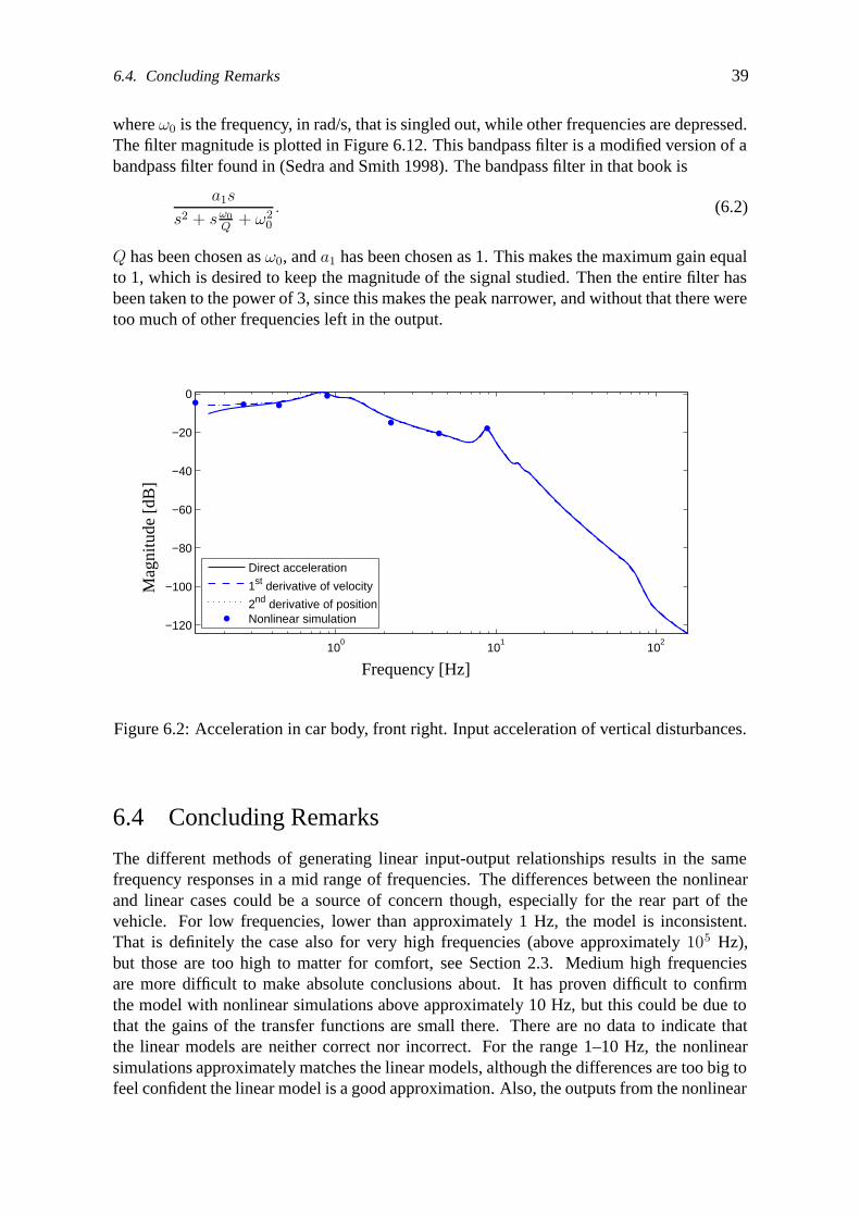
6.4. Concluding Remarks 39
where ω0 is the frequency, in rad/s, that is singled out, while other frequencies are depressed.The filter magnitude is plotted in Figure 6.12. This bandpass filter is a modified version of abandpass filter found in (Sedra and Smith 1998). The bandpass filter in that book is
a1s
s2 + sω0
Q+ ω2
0
. (6.2)
Q has been chosen as ω0, and a1 has been chosen as 1. This makes the maximum gain equalto 1, which is desired to keep the magnitude of the signal studied. Then the entire filter hasbeen taken to the power of 3, since this makes the peak narrower, and without that there weretoo much of other frequencies left in the output.
100
101
102
−120
−100
−80
−60
−40
−20
0
Direct acceleration
1st derivative of velocity
2nd derivative of positionNonlinear simulation
Mag
nitu
de[d
B]
Frequency [Hz]
Figure 6.2: Acceleration in car body, front right. Input acceleration of vertical disturbances.
6.4 Concluding Remarks
The different methods of generating linear input-output relationships results in the samefrequency responses in a mid range of frequencies. The differences between the nonlinearand linear cases could be a source of concern though, especially for the rear part of thevehicle. For low frequencies, lower than approximately 1 Hz, the model is inconsistent.That is definitely the case also for very high frequencies (above approximately 105 Hz),but those are too high to matter for comfort, see Section 2.3. Medium high frequenciesare more difficult to make absolute conclusions about. It has proven difficult to confirmthe model with nonlinear simulations above approximately 10 Hz, but this could be due tothat the gains of the transfer functions are small there. There are no data to indicate thatthe linear models are neither correct nor incorrect. For the range 1–10 Hz, the nonlinearsimulations approximately matches the linear models, although the differences are too big tofeel confident the linear model is a good approximation. Also, the outputs from the nonlinear
40 6. Frequency Range for Linear Model Validity
simulations were nonlinear, and needed to be filtered with a very narrow bandpass filter togive a linear output, which makes it even more difficult to make a comparison.
In brief, the linear model should not be used below 1 Hz or above 105 Hz. For 1–10 Hz, it seems reasonable to make an attempt to use the linear model. In the remainingfrequency interval, the model may or may not be sufficiently accurate. This means thatthe linear model is not suitable for studies of motion sickness, where low frequencies areimportant, see Section 2.3. For comfort studies, where the most interesting frequency regionis 2–40 Hz, with the peak at 6–10 Hz, it is more reasonable to use the linear model, althoughthere is some doubt about this usage also.

6.4. Concluding Remarks 41
100
101
102
−200
−150
−100
−50
0
50
Direct positionIntegrated velocity2 times integrated accelerationNonlinear simulation
Mag
nitu
de[d
B]
Frequency [Hz]
Figure 6.3: Deflection between car body and bogie frame, front right. Input acceleration ofvertical disturbances.
100
101
102
−120
−100
−80
−60
−40
−20
Direct acceleration
1st derivative of velocity
2nd derivative of positionNonlinear simulation
Mag
nitu
de[d
B]
Frequency [Hz]
Figure 6.4: Acceleration in car body, rear left. Input acceleration of vertical disturbances.

42 6. Frequency Range for Linear Model Validity
100
101
102
−300
−250
−200
−150
−100
−50
0
50
Direct positionIntegrated velocity2 times integrated accelerationNonlinear simulation
Mag
nitu
de[d
B]
Frequency [Hz]
Figure 6.5: Deflection between car body and bogie frame, rear left. Input acceleration ofvertical disturbances.
100
101
102
−115
−110
−105
−100
−95
−90
−85
−80
Direct acceleration
1st derivative of velocity
2nd derivative of position
Mag
nitu
de[d
B]
Frequency [Hz]
Figure 6.6: Acceleration in car body, front right. Input actuator force.
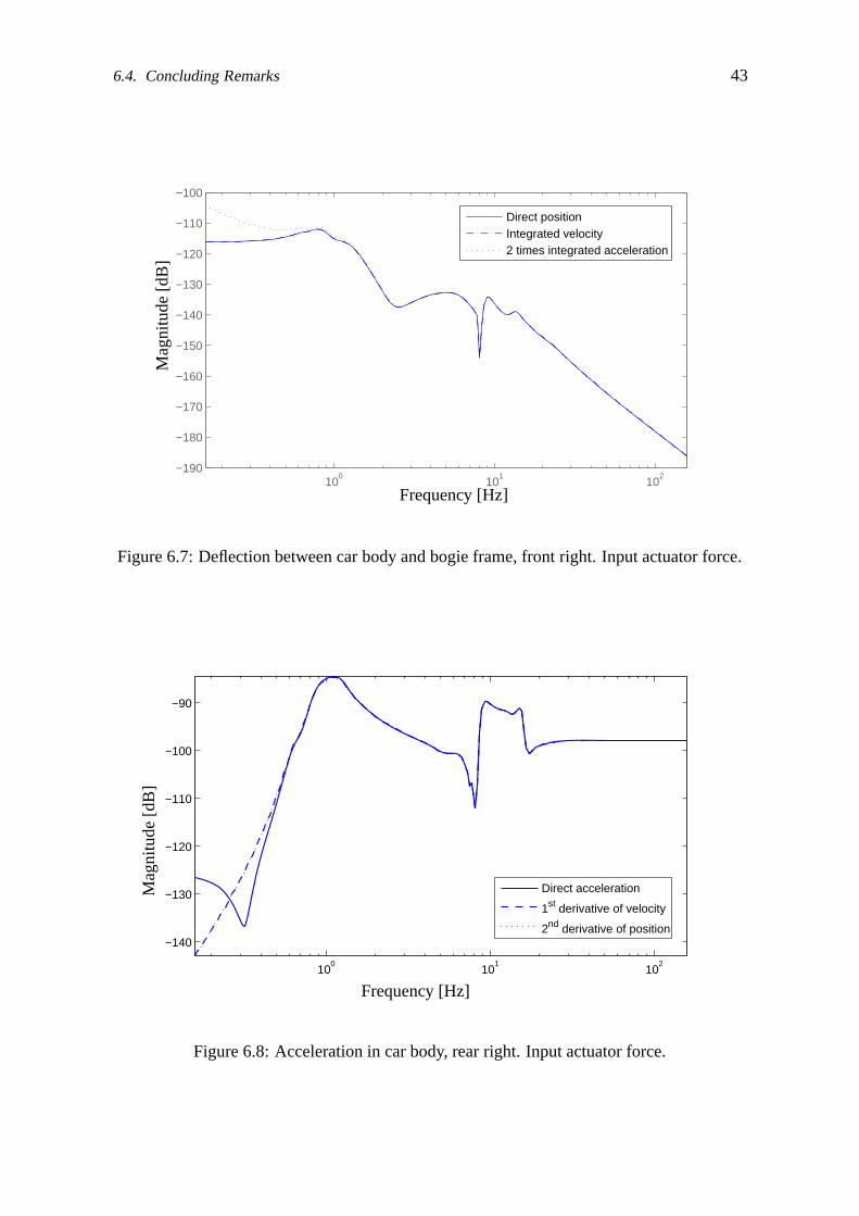
6.4. Concluding Remarks 43
100
101
102
−190
−180
−170
−160
−150
−140
−130
−120
−110
−100
Direct positionIntegrated velocity2 times integrated acceleration
Mag
nitu
de[d
B]
Frequency [Hz]
Figure 6.7: Deflection between car body and bogie frame, front right. Input actuator force.
100
101
102
−140
−130
−120
−110
−100
−90
Direct acceleration
1st derivative of velocity
2nd derivative of position
Mag
nitu
de[d
B]
Frequency [Hz]
Figure 6.8: Acceleration in car body, rear right. Input actuator force.

44 6. Frequency Range for Linear Model Validity
100
101
102
−220
−200
−180
−160
−140
−120
−100
Direct positionIntegrated velocity2 times integrated acceleration
Mag
nitu
de[d
B]
Frequency [Hz]
Figure 6.9: Deflection between car body and bogie frame, rear right. Input actuator force.
10−15
10−10
10−5
100
105
1010
−600
−400
−200
0
200
400
600
Direct acceleration
1st derivative of velocity
2nd derivative of position
Mag
nitu
de[d
B]
Frequency [Hz]
Figure 6.10: Acceleration in car body, front right. Input acceleration of vertical disturbances.All inputs in phase.

6.4. Concluding Remarks 45
10−10
10−5
100
105
1010
−1000
−500
0
500
1000
1500
Direct positionIntegrated velocity2 times integrated acceleration
Mag
nitu
de[d
B]
Frequency [Hz]
Figure 6.11: Deflection between car body and bogie frame, front right. Input acceleration ofvertical disturbances. All inputs in phase.
100
101
102
−180
−160
−140
−120
−100
−80
−60
−40
−20
0
Mag
nitu
de[d
B]
Frequency [Hz]
Figure 6.12: Bandpass filter used to get sinus from simulation output. Example forf0 = 4.4 Hz.


chapter vii
coupling between inputs and outputs
A single-input single-output (SISO) controller is easier to construct and analyze, and couldbe made less complex, than a multiple-input multiple-output (MIMO) controller. Therefore,it is interesting to study how each output depend on each input. It is also interesting to see ifthe system can be divided into smaller sub-systems.
The simplest solution would be, if one physical input (actuator force) could be connectedto the nearest output. That would allow for SISO design. If that is not possible, it might stillbe possible to decouple the system. That would also allow for SISO design, only the controland/or output signals used in the SISO design, would not correspond to any physical signal.Instead, they would have to be calculated from a combination of physical signals. It willhowever be shown below that neither version is possible.
7.1 Background Theory
This section describes formal methods to divide a system with multiple inputs and outputs,into several systems with a single input and output, for control purposes.
7.1.1 Relative Gain Array
To measure the amount of interaction between different inputs and output of a system, aspecial matrix called the Relative Gain Array, RGA, can be used, (Glad and Ljung 2000).For an arbitrary quadratic, invertible matrix A, this is defined as
RGA(A) = A. ∗ (A−1 )T , (7.1)
and for an arbitrary complex matrix A as
RGA(A) = A. ∗ (A† )T , (7.2)
where .* denotes elementwise multiplication, (Glad and Ljung 2000). In this chapter, RGAwill be used for the case when A = G(jω), where G(jω) is a matrix of transfer functions.
If RGA is used for a matrix of transfer functions, an input-output relation is not muchaffected by the other inputs, for RGA-elements near 1. If it is not near one for an output thatis supposed to be controlled by a certain input, there are significant cross couplings, (Gladand Ljung 2000). A perfectly decoupled system, where the inputs and outputs are numberedsuch that input number i controls output number i, for all i, has the unity matrix as its RGA,as can be seen from Equation 7.1.

48 7. Coupling Between Inputs and Outputs
7.1.2 The Pairing Problem
The pairing problem deals with deciding which output signals should be controlled by whichcontrol signals, (Glad and Ljung 2000). Two main rules are given in (Glad and Ljung 2000)to pair the signals using the RGA matrix.
1. Pair the signals in a way that will make the diagonal elements in RGA(G(jωc)), whereωc is the the intended bandwidth for the controlled system, as close to 1+0j as possible.
2. Avoid pairings that will make the diagonal elements in RGA(G(0)) negative.
When the relative gain is negative, there will be positive feedback in this loop, eitherwhen the other loops are open, or when they are closed, depending on controller configura-tion, (Shinskey 1996). Furthermore, if the relative gain is infinity, the loops are completelydependent, (Shinskey 1996).
7.1.3 Decoupling
If the inputs and outputs cannot be paired into pairs that dominate the dynamics, it might bepossible to use variable changes to find such pairs, (Glad and Ljung 2000). Let y = W2y andu = W−1
1 u. Then the transfer function from u to y will be
G(s) = W2(s)G(s)W1(s). (7.3)
W1 and W2 should be chosen to make G(s) as diagonal as possible, which would make itpossible to make a diagonal controller F diag
y for the new variables, (Glad and Ljung 2000).In the original variables the controller will then be
u = −W1Fdiagy W2y, (7.4)
which is a decoupled controller, (Glad and Ljung 2000).To get the system truly decoupled (diagonal), the matrices W1 and W2 would have to
be complex and dynamic (depending on s). Normally, this cannot be implemented, and thusconstant, real matrices have to be used instead as an approximation. This approximation ismade by choosing a frequency at which the decoupling is made, (Glad and Ljung 2000).
7.2 Signal Coupling and Pairing
To pair each input with one output it is necessary to have the same number of outputs andinputs. (The input and outputs and their numbering were described in Section 4.1.3.) Asthe main choice, only the acceleration outputs are chosen. This is since the accelerations arethe outputs that are related to comfort, which is what is aimed at to optimize in this thesis,see Section 3.1. Since deflection would have to be kept under control, some other controllaw would have to be superimposed to keep it within boundaries, though. Therefore, thecoupling of the deflections are also studied.

7.2. Signal Coupling and Pairing 49
7.2.1 Gain Plots
In this subsection gains between inputs and outputs are plotted. If one output is influencedmuch more by one input than by the others, the gain from that input will be much larger, andwill be a natural choice for SISO pairing. The advantage of using this method, compared tousing the RGA as in the next subsection, is that the entire interesting frequency range can bestudied at once. Thus, the risk of not noticing interaction that is limited to a small frequencyrange, is minimized.
To allow comparison, the magnitudes of the transfer functions from input number i tooutput number k, Gik, have been plotted in Figure 7.1–Figure 7.2. Then, to make it easierto see how much the actuators influence the output relative to each other, the quotient of thegains have been calculated. Those quotients, plotted in Figure 7.3–Figure 7.6, are calculatedas
Grel,ik(jω) =|Gik(jω)||Gkk(jω)| . (7.5)
When i = k it is the same function in the numerator as in the denominator. Thus the valueof Grel,ik(jω) is 1 for all ω. This is the transfer function from the actuator closest to themeasured output, which is the most natural choice of input-output pairing. That is, the inputactuator force, front right, is paired with the output car body acceleration, front right, andso on. It is desirable that the transfer functions from the other actuators to the same outputare small. However, as can be seen in Figure 7.3–Figure 7.6, they are not. In some casesthere are some frequency ranges in which they are even higher. The influence from otheractuators are thus substantial, and could hardly be neglected. This is true also when interestis directed to only the most important region, which would be approximately 2–40 Hz forthe acceleration, according to Figure 2.3, or maybe with an upper limit for model validityat 10 Hz according to the discussion in Section 6. The locations of inputs and outputs areillustrated in Figure 4.2. The vehicle is almost symmetric, and the plots for left and right sideare almost identical. Therefore only one side is plotted.
The reason for plotting both Gik(jω) and Grel,ik(jω) is that studying both those simul-taneously makes it easier to see if there are significant interaction from other actuators thanthe one that is supposed to control a certain output. It is easier to see the relative influencesin Grel,ik(jω), but if the coupling is strong only where the magnitude Gik(jω) has a notchfrequency, it might be of less importance, or even due to numerical errors. The highest, sharppeak in Figure 7.3 admittedly is at the frequency where there is a notch in the gain (see Fig-ure 7.1), but there are comparatively high influence from other actuators also at frequencieswhere the gain is high.
7.2.2 Relative Gain Array
A more formal way to show that there is no way to pair the inputs and outputs into SISO con-trolled loops is by using the relative gain array (RGA). The relative gain array is calculatedaccording to Section 7.1.1. (All the cases below turn out to have full rank. Thus the inverseexists, and is therefore used in the equations.) Relative gain arrays are calculated at steadystate as well as two different suggested bandwidths (10 Hz and 40 Hz). This since those areneeded to make the pairing according to Section 7.1.2. RGA has also been calculated for5 Hz, since this is about in the middle of the most interesting frequency region. If the systemis split into SISO systems, it is important to know that nothing strange happens there.

50 7. Coupling Between Inputs and Outputs
When accelerations are used as outputs the following relative gain arrays are obtained:
RGA(G(0)) = 107 ·
⎛⎜⎜⎜⎜⎜⎜⎝
-4.2 5.4 -5.6 4.5
4.3 -5.5 5.8 -4.6
3.4 -4.3 4.5 -3.6
-3.5 4.4 -4.7 3.7
⎞⎟⎟⎟⎟⎟⎟⎠
(7.6)
RGA(G(5 · 2πj)) = 1010 ·
⎛⎜⎜⎜⎜⎜⎜⎝
-6.4-28j 5.6+22j 1.9-1.6j -1.1+7.5j
5.6+22j -6.4-28j -1.0+7.5j 1.9-1.5j
-1.0-5.5j 1.8+11j 1.6-16j -2.5+9.8j
1.8+11j -1.0-5.5j -2.5+9.8j 1.7-1.6j
⎞⎟⎟⎟⎟⎟⎟⎠
(7.7)
RGA(G(10·2πj)) = 1011 ·
⎛⎜⎜⎜⎜⎜⎜⎝
4.0+5.3j -3.7-4.78j 1.1+1.2j -1.4-1.7j
-3.7-4.8j 4.0+5.3j -1.4-1.7j 1.1+1.2j
1.2+1.7j -1.5-2.2j 3.8+3.8j -3.4-3.3j
-1.5-2.2j 1.2+1.7j -3.4-3.3j 3.8+3.8j
⎞⎟⎟⎟⎟⎟⎟⎠
(7.8)
RGA(G(40 · 2πj)) = 1012 ·
⎛⎜⎜⎜⎜⎜⎜⎝
-9.1+19j 7.3-15j -1.5+3.1j 3.3-6.9j
7.3-15j -9.1+19j 3.3-6.9j -1.5+3.1j
-1.5+3.2j 3.3-6.9j -9.1+19j 7.2-15j
3.3-6.9j -1.5+3.2j 7.2-15j -9.1+19j
⎞⎟⎟⎟⎟⎟⎟⎠(7.9)
In the matrices above it is clearly seen that no element is anywhere near 1, which was neededfor pairing. Instead, they are very large, which means that the loops are very dependent ofeach other. Thus, there is no pairing possible. This is the same conclusion as in the previoussection, where the same interactions were studied in a different way.
When deflections are used as outputs the following relative gain arrays are obtained:
RGA(G(0)) =
⎛⎜⎜⎜⎜⎜⎜⎝
4.4 -3.2 -0.05 -0.1
-3.3 4.4 -0.09 -0.05
0.0001 -0.15 4.6 -3.4
-0.15 0.007 -3.4 4.6
⎞⎟⎟⎟⎟⎟⎟⎠
(7.10)

7.2. Signal Coupling and Pairing 51
RGA(G(5 · 2πj)) =⎛⎜⎜⎜⎜⎜⎜⎝
1.3-0.65j -0.26+0.65j -0.0006+0.0001j 0.001-0.001j
-0.26+0.65j 1.3-0.65j 0.001-0.001j 0.0006+0.0001j
-0.0007+0.0003j 0.001-0.001j 1.3-0.66j -0.31+0.67j
0.001-0.001j -0.0007+0.0003j -0.31+0.67j 1.3-0.66j
⎞⎟⎟⎟⎟⎟⎟⎠
(7.11)
RGA(G(10 · 2πj)) =⎛⎜⎜⎜⎜⎜⎜⎝
0.63-0.67j 0.38+0.67j -0.002-0.001j -0.002+0.0002j
0.38+0.67j 0.63-0.67j -0.002+0.0002j -0.002-0.001j
-0.002-0.001j -0.002+0.0002j 0.89-0.55j 0.12+0.55j
-0.002+0.0002j -0.002-0.001j 0.12+0.55j 0.89-0.55j
⎞⎟⎟⎟⎟⎟⎟⎠
(7.12)
RGA(G(40 · 2πj)) =⎛⎜⎜⎜⎜⎜⎜⎝
1.0-0.002j -0.002+0.002j -0.0005 -0.002
-0.002+0.002j 1.0-0.002j -0.002 -0.0005
-0.0005 -0.002 1.0-0.0006j 0.001+0.0006j
-0.002 -0.0005 0.001+0.0006j 1.0-0.0006j
⎞⎟⎟⎟⎟⎟⎟⎠
(7.13)
This is better than for acceleration, since those are much close to the identity matrix, andin all cases the numbers on the diagonal are positive. Here, if studying only those RGA:s,chosen according to the suggestions in Section 7.1.1, it would be possible to pair the signalsaccording to the rules in that same section. Then input number 1 would be paired with outputnumber 1, 2 with 2, 3 with 3 and 4 with 4. That means that each actuator would control theoutput closest to itself, see Chapter 4.1. The interaction from the nearest actuator is howeverhigh at low and medium frequencies. Therefore it might be better to divide the system intotwo 2×2 systems. However, as already mentioned, neither solution would be able to controlthe acceleration, which is important to comfort. Therefore, such a solution is impossible forthe purposes of this thesis.
The conclusion that if only deflections were interesting, it would be possible to dividethe system into two 2 × 2 systems, is not the same as in the previous subsection. StudyingFigure 7.4 and Figure 7.6 tells us that there are quite a lot of influences from all actuators atsome frequencies. Looking at those figures, for instance 1 Hz could be interesting to study.

52 7. Coupling Between Inputs and Outputs
Now we get
RGA(G(1 · 2πj)) =
⎛⎜⎜⎜⎜⎜⎜⎝
2.2-4.4j -1.4+4.3j 1.6-0.93j -1.4+0.96j
-1.4+4.3j 2.3-4.4j -1.4+0.98j 1.6-0.91j
1.5-0.79j -1.3+0.82j 1.0-5.0j -0.19+5.0j
-1.3+0.84j 1.4-0.77j -0.18+5.0j 1.0-5.1j
⎞⎟⎟⎟⎟⎟⎟⎠
.
(7.14)
Here it is no longer obvious which actuator should control which output. The influencesare high not only between left and right side, but also between front and rear bogie. Thisexample serves as a warning to accept a pairing suggested by the RGA without checkingintermediate frequencies.
7.3 Decoupling
Since input-output pairing didn’t work, an attempt is made at decoupling. An attempt ismade at exact decoupling at a single frequency. That is, complex matrices has been allowed.According to Section 7.1, normally real matrices are needed for implementation. Such ap-proximations have not been reported here, since already the complex decoupling matriceshave been found insufficient, as seen below. The weighing matrices W1 and W2 have beenchosen as G(jωdc)
−1 and the identity matrix, respectively, inspired by an example in (Gladand Ljung 2000). This corresponds to weighing of the input (control) signal. ωdc is the fre-quency that is chosen for decoupling, here 5 · 2π rad/s (5 Hz). The inverse of G does existat this frequency. With those choices of weighing matrices, the decoupled system, G(jω),will be the identity matrix at ωdc. Thus G(jωdc) is perfectly diagonal, as desired. With thischoice, also RGA(G(jωdc)) will be unity. The system is perfectly decoupled at the selectedfrequency. However, even a minor change in frequency will make the system heavily cou-pled again. Shown below is the RGA for 4.9 Hz, where we even get negative elements onthe diagonal, which indicates positive feedback.
RGA(G(4.9 · 2πj)) = 1013 ·
⎛⎜⎜⎜⎜⎜⎜⎝
-1.4-1.4j -0.89-1.5j 0.46+1.6j 1.8+1.3j
-0.9-1.6j -0.47-1.6j 0.05+1.6j 1.4+1.6j
0.55+1.8j 0.09+1.6j 0.32-1.6j -0.97-1.8j
1.8+1.2j 1.3+1.4j -0.82-1.7j -2.2-1.0j
⎞⎟⎟⎟⎟⎟⎟⎠
(7.15)
Similarly, for decoupling at 2 Hz. The decoupling is perfect at 2 Hz, but unacceptableat 1.9 Hz, see below.
RGA(G(1.9·2πj)) = 1013·
⎛⎜⎜⎜⎜⎜⎜⎝
1.0-0.34j 1.0-0.31j -1.0+0.30j -1.0+0.35j
1.0-0.31j 1.1-0.28j -1.1+0.26j -1.0+0.32j
-1.0+0.30j -1.1+0.27j 1.1-0.25j 1.0-0.31j
-1.0+0.35j -1.1+0.32j 1.0-0.31j 1.0-0.36j
⎞⎟⎟⎟⎟⎟⎟⎠
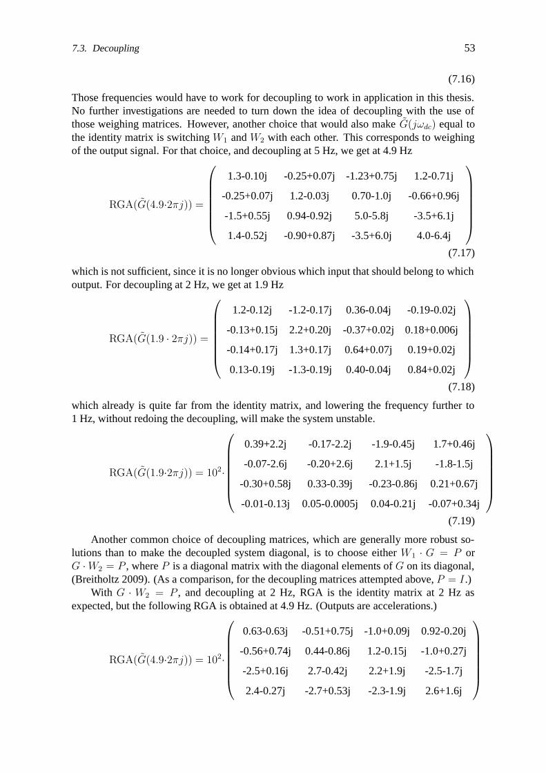
7.3. Decoupling 53
(7.16)
Those frequencies would have to work for decoupling to work in application in this thesis.No further investigations are needed to turn down the idea of decoupling with the use ofthose weighing matrices. However, another choice that would also make G(jωdc) equal tothe identity matrix is switching W1 and W2 with each other. This corresponds to weighingof the output signal. For that choice, and decoupling at 5 Hz, we get at 4.9 Hz
RGA(G(4.9·2πj)) =
⎛⎜⎜⎜⎜⎜⎜⎝
1.3-0.10j -0.25+0.07j -1.23+0.75j 1.2-0.71j
-0.25+0.07j 1.2-0.03j 0.70-1.0j -0.66+0.96j
-1.5+0.55j 0.94-0.92j 5.0-5.8j -3.5+6.1j
1.4-0.52j -0.90+0.87j -3.5+6.0j 4.0-6.4j
⎞⎟⎟⎟⎟⎟⎟⎠
(7.17)
which is not sufficient, since it is no longer obvious which input that should belong to whichoutput. For decoupling at 2 Hz, we get at 1.9 Hz
RGA(G(1.9 · 2πj)) =
⎛⎜⎜⎜⎜⎜⎜⎝
1.2-0.12j -1.2-0.17j 0.36-0.04j -0.19-0.02j
-0.13+0.15j 2.2+0.20j -0.37+0.02j 0.18+0.006j
-0.14+0.17j 1.3+0.17j 0.64+0.07j 0.19+0.02j
0.13-0.19j -1.3-0.19j 0.40-0.04j 0.84+0.02j
⎞⎟⎟⎟⎟⎟⎟⎠
(7.18)
which already is quite far from the identity matrix, and lowering the frequency further to1 Hz, without redoing the decoupling, will make the system unstable.
RGA(G(1.9·2πj)) = 102·
⎛⎜⎜⎜⎜⎜⎜⎝
0.39+2.2j -0.17-2.2j -1.9-0.45j 1.7+0.46j
-0.07-2.6j -0.20+2.6j 2.1+1.5j -1.8-1.5j
-0.30+0.58j 0.33-0.39j -0.23-0.86j 0.21+0.67j
-0.01-0.13j 0.05-0.0005j 0.04-0.21j -0.07+0.34j
⎞⎟⎟⎟⎟⎟⎟⎠
(7.19)
Another common choice of decoupling matrices, which are generally more robust so-lutions than to make the decoupled system diagonal, is to choose either W1 · G = P orG · W2 = P , where P is a diagonal matrix with the diagonal elements of G on its diagonal,(Breitholtz 2009). (As a comparison, for the decoupling matrices attempted above, P = I .)
With G · W2 = P , and decoupling at 2 Hz, RGA is the identity matrix at 2 Hz asexpected, but the following RGA is obtained at 4.9 Hz. (Outputs are accelerations.)
RGA(G(4.9·2πj)) = 102·
⎛⎜⎜⎜⎜⎜⎜⎝
0.63-0.63j -0.51+0.75j -1.0+0.09j 0.92-0.20j
-0.56+0.74j 0.44-0.86j 1.2-0.15j -1.0+0.27j
-2.5+0.16j 2.7-0.42j 2.2+1.9j -2.5-1.7j
2.4-0.27j -2.7+0.53j -2.3-1.9j 2.6+1.6j
⎞⎟⎟⎟⎟⎟⎟⎠

54 7. Coupling Between Inputs and Outputs
(7.20)
Here the elements are large and it is also unclear which input-output pairs are dominating.Thus this decoupling matrix did not work either.
A final attempt is made with W1 · G = P . With decoupling at 2 Hz, we get already at1.9 Hz:
RGA(G(1.9 · 2πj)) = 1012 ·
⎛⎜⎜⎜⎜⎜⎜⎝
-1.2+2.0j -1.3+2.0j 1.3-2.0j 1.2-2.0j
-1.3+2.0j -1.4+2.0j 1.4-2.0j 1.3-2.0j
1.3-2.0j 1.4-2.0j -1.4+1.9j -1.3+2.0j
1.2-2.0j 1.3-2.0j -1.3+2.0j -1.2+2.1j
⎞⎟⎟⎟⎟⎟⎟⎠
(7.21)
This is very large and the loops are therefore almost completely dependent.The conclusion is that decoupling does not work with neither input nor output weighing,
for any of the decoupling matrices studied for this system. Generally the output weighing de-teriorates slower though, as the RGA is studied further away from the decoupling frequency.
7.4 Concluding Remarks
Unfortunately the coupling between all input-to-output relations is very high, and no pairingthat can be used for control design can be found. Decoupling with stationary weight matricesdoes not look promising either, not even over a small frequency interval. This is probablydue to the strong frequency dependence of the coupling. Therefore, MIMO design has beenchosen.

7.4. Concluding Remarks 55
100
101
102
−140
−130
−120
−110
−100
−90
−80
−70
Front rightFront leftRear rightRear left
Mag
nitu
de[d
B((
m/s
2)/
N)]
Frequency [Hz]
Figure 7.1: Gain plot of transfer function from all actuator forces to acceleration in car body,front right. Train velocity 1 km/h, passive suspension.
100
101
102
−220
−200
−180
−160
−140
−120
−100
Front rightFront leftRear rightRear left
Mag
nitu
de[d
B(m
/N)]
Frequency [Hz]
Figure 7.2: Gain plot of transfer function from all actuator forces to bogie-to-carbody de-flection, rear right. Train velocity 1 km/h, passive suspension.

56 7. Coupling Between Inputs and Outputs
100
101
102
0
0.2
0.4
0.6
0.8
1
1.2
Front rightFront leftRear rightRear left
Frequency [Hz]
Rel
ativ
ega
in
Figure 7.3: Magnitude of transfer function from each actuator (force) to car body accel-eration front right, divided by magnitude of transfer function from the front right actuator.Normalized according to Equation 7.5.

7.4. Concluding Remarks 57
100
101
102
0
0.2
0.4
0.6
0.8
1
Front rightFront leftRear rightRear left
Frequency [Hz]
Rel
ativ
ega
in
Figure 7.4: Magnitude of transfer function from each actuator (force) to bogie-to-carbodydeflection front right, divided by magnitude of transfer function from the front right actuator.Normalized according to Equation 7.5.

58 7. Coupling Between Inputs and Outputs
100
101
102
0
0.2
0.4
0.6
0.8
1
Front rightFront leftRear rightRear left
Frequency [Hz]
Rel
ativ
ega
in
Figure 7.5: Magnitude of transfer function from each actuator (force) to car body accel-eration rear right, divided by magnitude of transfer function from the rear right actuator.Normalized according to Equation 7.5.
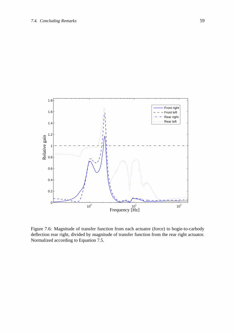
7.4. Concluding Remarks 59
100
101
102
0
0.2
0.4
0.6
0.8
1
1.2
1.4
1.6
1.8
Front rightFront leftRear rightRear left
Frequency [Hz]
Rel
ativ
ega
in
Figure 7.6: Magnitude of transfer function from each actuator (force) to bogie-to-carbodydeflection rear right, divided by magnitude of transfer function from the rear right actuator.Normalized according to Equation 7.5.

chapter viii
model reduction
Since Chapter 7 showed that SISO control design wasn’t feasible, the choice will have tofall on MIMO control design. Modern methods of controller design, such as H∞ and LQG,produce controllers of equal or higher order than the plant, (Skogestad and Postlethwaite1996). (Both H∞ and LQG are methods that can be used with MIMO systems, (Glad andLjung 2000).) If a system can be approximated with one of a lower order, it makes analysis,control design, and implementation easier, (Glad and Ljung 2000).
This approximation is what is referred to as model reduction or model simplification.One starts with a higher order model, and reduces it to a model with a lower order than theinitial model.
Assuming that not all states can be measured, it is necessary to use an observer if somekind of state feedback is to be used. (Which is the case for instance when using LQ control.)The Kalman filter requires a model both from disturbances and control signals (with thesame states and outputs), (The MathWorks 2007). Thus the goal of the model reduction isto calculate a reduced model from both the control signals and disturbances, with both thesame states and outputs. The models should be as much reduced as possible while still being“good enough”.
In this chapter an algorithm, tailored for model reduction of the railway vehicle modelstudied in this thesis, is developed and compared with two commercial methods. The modelused as a starting point for all reductions in this chapter, is a linear time-invariant model onstate space form, the same as in Chapter 6.
8.1 Background Theory
This section describes commercial methods of model reduction and their basis, as well as thetheoretical basis for another method suggested in this chapter.
Assume a system on the following form:
x = Ax + Bu (8.1)
y = Cx + Du, (8.2)
where x represents the states, u the inputs, and y the outputs.

62 8. Model Reduction
8.1.1 State Transform
With the state transform ξ = Tx, if the inverse of T exists, the state space model will turninto
ξ = TAT−1ξ + TBu (8.3)
y = CT−1ξ + Du, (8.4)
(Lennartson 2002).
8.1.2 Diagonalization
An n×n matrix A is diagonalizable if and only if A has n linearly independent eigenvectors.If it is diagonalizable it can be written on the form A = vAdiagv
−1, where v is an n×n-matrixconsisting of the eigenvectors to the diagonal matrix Adiag , (Bengtsson and Weisstein 2008).
8.1.3 Controllability and Observability
A state vector x∗ is controllable if there is an input signal that brings the state from the originto x∗ in finite time. A system is controllable if all its state vectors are controllable. A statevector x∗ �= 0 is unobservable if the output signal is identically zero when the initial valueis x∗ and the input signal is identically zero. The system is observable if none of its statevectors are unobservable, (Glad and Ljung 1989).
When a system is on a diagonal form, a mode xi with corresponding row vector Bi = 0is not affected by the input, and is thus uncontrollable, (Glad and Ljung 2000). In the sameway, a mode xi with corresponding column vector Ci = 0, does not affect the output, and isthus unobservable, (Glad and Ljung 2000).
The Controllability Gramian can be written as
Sx =
∫ ∞
0
eAtBBT eAT tdt, (8.5)
and the Observability Gramian as
Ox =
∫ ∞
0
eAT tCT CeAtdt, (8.6)
(Glad and Ljung 2000)
8.1.4 Balanced Realization
A balanced realization is an asymptotically stable minimal realization in which the control-lability and observability Gramians are equal and diagonal, (Skogestad and Postlethwaite1996).
8.1.5 Softwares for Model Simplification
Two software programs with support for model simplification, both based on balancing tech-niques, have been used. Those are briefly described below.

8.2. Evaluation Method 63
Slicot
SLICOT is a subroutine library based on BLAS and LAPACK routines and further devel-oped, partly in the framework of the European project NICONET1, (Benner et al. 1998). TheSLICOT routines are written in Fortran 77, but they can also run from Matlab and Scilab,(Varga 2000).
According to the Slicot manual, its command fwbred is a function for frequency-weighted balancing related model reduction. It has support for input and output weigh-ing. fwbred also handles unstable models, and will then always keep the unstable parts,(Niconet 2005). There are two methods available for the reduction: the Balanced TruncationApproximation and the Singular Perturbation Approximation, (Niconet 2005).
Matlab
In a paper published the year 2000, (Varga 2000), Varga showed that balreal, which is amethod for balanced realization in Matlab that is used for model reduction, systematicallyfails at high order systems, which Slicot handles. However, since this paper was published,Mathworks have improved their algorithms. It still indicates that there are numerical issuesto deal with when reducing large models, though.
According to the Matlab manual, its command balred uses implicit balancing tech-niques to compute a reduced-order approximation. balred also handles unstable models,and will then always keep the unstable parts, (The MathWorks 2007). As opposed to the Sli-cot routine described above, there is however no support for neither input nor output weigh-ing. With balred, there are two choices of how to reduce the model. One is to enforcematching DC gains, and the other to discard the states associated with small Hankel singularvalues. The latter method, that is referred to as the ’Truncate’ method, tends to produce abetter approximation in the frequency domain, but the DC gains are not guaranteed to match,(The MathWorks 2007).
8.2 Evaluation Method
The reduced model is good enough if it can be used to design a controller which, with anacceptable outcome, can be placed in the un-reduced model. This is difficult to see withoutactually doing so, but there are some indications. The un-reduced and reduced models arecompared in Bode plots. The Bode plots where the outputs are accelerations are multipliedwith the comfort filter, described in Section 2.3, before evaluation. The reason for this is thatcomfort is one of the evaluation criterions, which acceleration in itself isn’t, see Section 3.1.If the frequency weighted Bode plots from the reduced model seem to follow the unreducedrather well in the selected area, 1–40 Hz, the reduced model is a candidate for controllerdesign. The frequency range is chosen based on the vertical comfort filter in Section 2.3, andthe frequency range of model validity in Chapter 6, with some added margin in the upperfrequency region.
The Bode plots are compared for accurateness using visual inspection. More weight isput on the control signal to output relationship, than to the disturbance to output relationship.The reason for this is that if you cannot control a state it does not help much to model it.Also, there could be other, unknown, disturbances not modeled.
1http://www.win.tue.nl/niconet/niconet.html
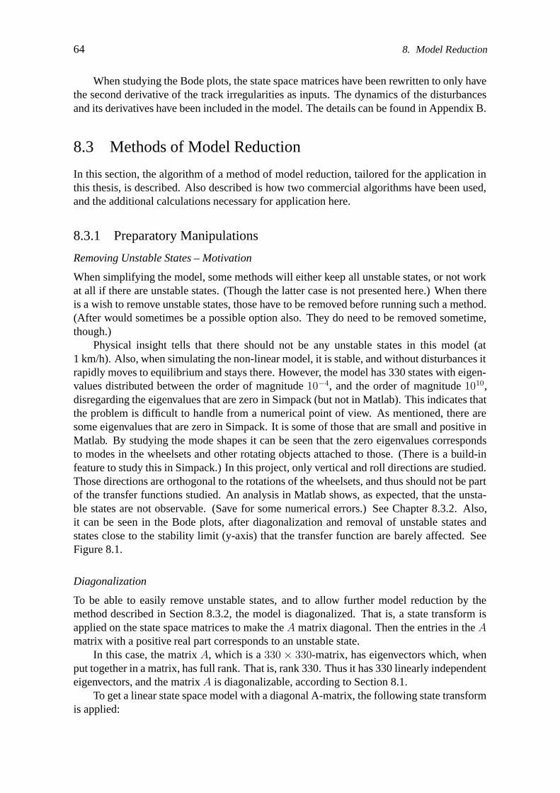
64 8. Model Reduction
When studying the Bode plots, the state space matrices have been rewritten to only havethe second derivative of the track irregularities as inputs. The dynamics of the disturbancesand its derivatives have been included in the model. The details can be found in Appendix B.
8.3 Methods of Model Reduction
In this section, the algorithm of a method of model reduction, tailored for the application inthis thesis, is described. Also described is how two commercial algorithms have been used,and the additional calculations necessary for application here.
8.3.1 Preparatory Manipulations
Removing Unstable States – Motivation
When simplifying the model, some methods will either keep all unstable states, or not workat all if there are unstable states. (Though the latter case is not presented here.) When thereis a wish to remove unstable states, those have to be removed before running such a method.(After would sometimes be a possible option also. They do need to be removed sometime,though.)
Physical insight tells that there should not be any unstable states in this model (at1 km/h). Also, when simulating the non-linear model, it is stable, and without disturbances itrapidly moves to equilibrium and stays there. However, the model has 330 states with eigen-values distributed between the order of magnitude 10−4, and the order of magnitude 1010,disregarding the eigenvalues that are zero in Simpack (but not in Matlab). This indicates thatthe problem is difficult to handle from a numerical point of view. As mentioned, there aresome eigenvalues that are zero in Simpack. It is some of those that are small and positive inMatlab. By studying the mode shapes it can be seen that the zero eigenvalues correspondsto modes in the wheelsets and other rotating objects attached to those. (There is a build-infeature to study this in Simpack.) In this project, only vertical and roll directions are studied.Those directions are orthogonal to the rotations of the wheelsets, and thus should not be partof the transfer functions studied. An analysis in Matlab shows, as expected, that the unsta-ble states are not observable. (Save for some numerical errors.) See Chapter 8.3.2. Also,it can be seen in the Bode plots, after diagonalization and removal of unstable states andstates close to the stability limit (y-axis) that the transfer function are barely affected. SeeFigure 8.1.
Diagonalization
To be able to easily remove unstable states, and to allow further model reduction by themethod described in Section 8.3.2, the model is diagonalized. That is, a state transform isapplied on the state space matrices to make the A matrix diagonal. Then the entries in the Amatrix with a positive real part corresponds to an unstable state.
In this case, the matrix A, which is a 330 × 330-matrix, has eigenvectors which, whenput together in a matrix, has full rank. That is, rank 330. Thus it has 330 linearly independenteigenvectors, and the matrix A is diagonalizable, according to Section 8.1.
To get a linear state space model with a diagonal A-matrix, the following state transformis applied:

8.3. Methods of Model Reduction 65
Anew = v−1Aoldv (8.7)
Bnew = v−1Bold (8.8)
Cnew = Coldv (8.9)
Dnew = Dold. (8.10)
In practice though, the eigenvector matrix v and the diagonal matrix Adiag with eigen-values on the diagonal, are calculated simultaneously with the Matlab command eig. Anew
is set to be Adiag . This way Anew will really be diagonal, and round-off errors on the off-diagonal elements will be avoided. In theory Adiag = v−1Aoldv.
State Removal
Since the system is now on diagonal form, the rows and columns corresponding to a certainstate, that has been found unimportant, can simply be deleted. This is also the method chosen.Another choice would have been to match the DC-gain (0 Hz), but this worsens the accuracyin other frequency intervals. The DC-gain is not considered the primary concern here, sinceif needed that could be taken care of by a slower loop containing integration, acting on theerror in the outputs. Also, it is outside of the chosen range, as mentioned above. And as seenin Chapter 6, the model is not valid below 1 Hz anyway.
8.3.2 Tailored Algorithm
When using the tailored algorithm described here, the model is reduced based on a combina-tion of observability, controllability from the actuators and (sometimes) controllability fromthe disturbances, as well as frequency concerns.
The original reason for developing a tailored algorithm was that the balancing methodsin Matlab could not handle sufficiently large models. After improvements in recent versionsof Matlab, Matlab’s build-in functions for model reduction can be used. The algorithmdescribed here yields significantly better results, though. See Section 8.4.
An overview of the tailored algorithm can be found in Figure 8.2. A more detaileddescription can be found in the enumerated list that follows. For clarifying reasons, theinputs have been divided into control inputs u, and disturbance inputs w. The syntax used is
x = Ax + Bu + Nw (8.11)
y = Cx + Du + Mw. (8.12)
1. To make it easy to see which states corresponds to high frequencies and which arecontrollable or observable, the model is written on diagonal form, as described inSection 8.3.1. Then the eigenvalues can be found on the diagonal.
2. Then, parts of the state space representation that correspond to high frequencies areselected for removal. Those are selected since the high frequency accelerations are notimportant for human comfort, and the deflections are small in those regions anyway.The choice has fallen on removing states with eigenvalues corresponding to frequen-cies higher than 40 Hz.
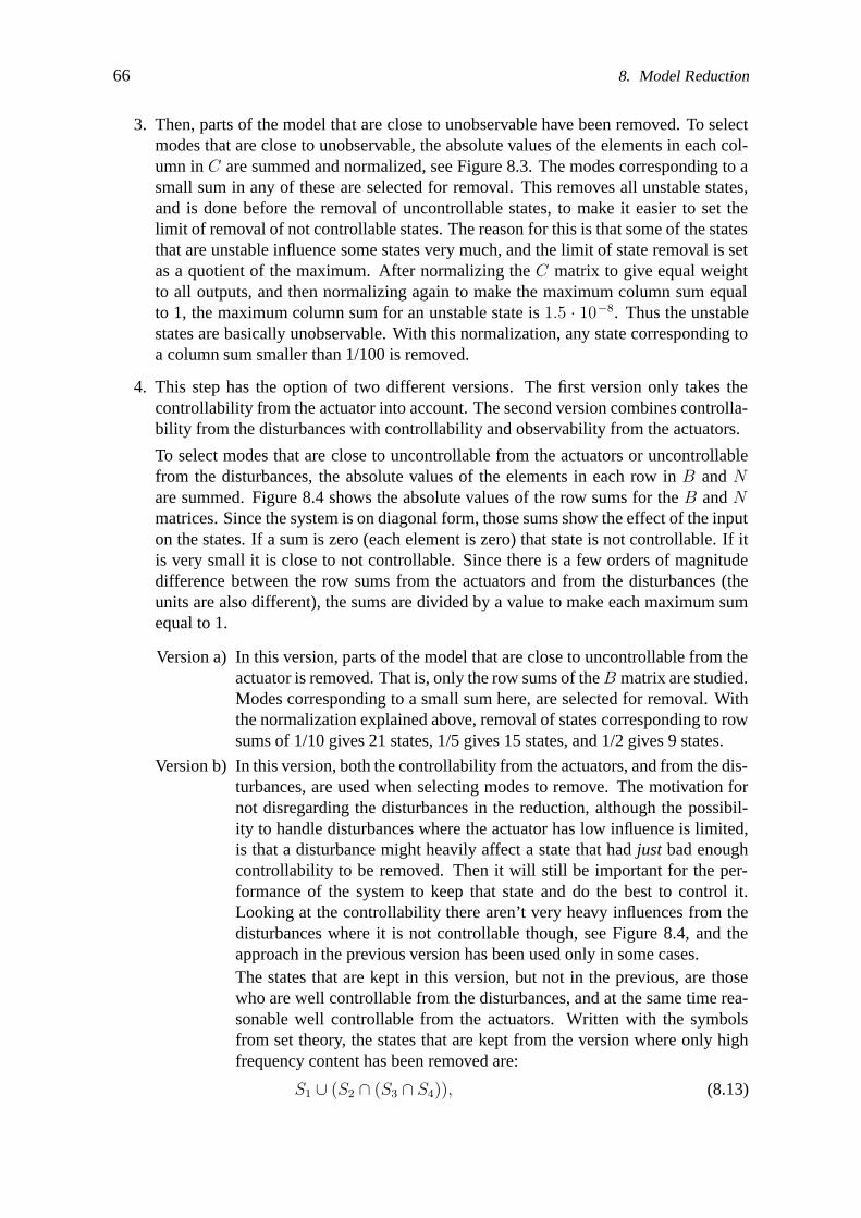
66 8. Model Reduction
3. Then, parts of the model that are close to unobservable have been removed. To selectmodes that are close to unobservable, the absolute values of the elements in each col-umn in C are summed and normalized, see Figure 8.3. The modes corresponding to asmall sum in any of these are selected for removal. This removes all unstable states,and is done before the removal of uncontrollable states, to make it easier to set thelimit of removal of not controllable states. The reason for this is that some of the statesthat are unstable influence some states very much, and the limit of state removal is setas a quotient of the maximum. After normalizing the C matrix to give equal weightto all outputs, and then normalizing again to make the maximum column sum equalto 1, the maximum column sum for an unstable state is 1.5 · 10−8. Thus the unstablestates are basically unobservable. With this normalization, any state corresponding toa column sum smaller than 1/100 is removed.
4. This step has the option of two different versions. The first version only takes thecontrollability from the actuator into account. The second version combines controlla-bility from the disturbances with controllability and observability from the actuators.
To select modes that are close to uncontrollable from the actuators or uncontrollablefrom the disturbances, the absolute values of the elements in each row in B and Nare summed. Figure 8.4 shows the absolute values of the row sums for the B and Nmatrices. Since the system is on diagonal form, those sums show the effect of the inputon the states. If a sum is zero (each element is zero) that state is not controllable. If itis very small it is close to not controllable. Since there is a few orders of magnitudedifference between the row sums from the actuators and from the disturbances (theunits are also different), the sums are divided by a value to make each maximum sumequal to 1.
Version a) In this version, parts of the model that are close to uncontrollable from theactuator is removed. That is, only the row sums of the B matrix are studied.Modes corresponding to a small sum here, are selected for removal. Withthe normalization explained above, removal of states corresponding to rowsums of 1/10 gives 21 states, 1/5 gives 15 states, and 1/2 gives 9 states.
Version b) In this version, both the controllability from the actuators, and from the dis-turbances, are used when selecting modes to remove. The motivation fornot disregarding the disturbances in the reduction, although the possibil-ity to handle disturbances where the actuator has low influence is limited,is that a disturbance might heavily affect a state that had just bad enoughcontrollability to be removed. Then it will still be important for the per-formance of the system to keep that state and do the best to control it.Looking at the controllability there aren’t very heavy influences from thedisturbances where it is not controllable though, see Figure 8.4, and theapproach in the previous version has been used only in some cases.The states that are kept in this version, but not in the previous, are thosewho are well controllable from the disturbances, and at the same time rea-sonable well controllable from the actuators. Written with the symbolsfrom set theory, the states that are kept from the version where only highfrequency content has been removed are:
S1 ∪ (S2 ∩ (S3 ∩ S4)), (8.13)

8.3. Methods of Model Reduction 67
where S1 contains the states that are well controllable from the control sig-nals, S2 contains the states that are well controllable from the disturbancesignals, S3 contains the states that are reasonable well controllable fromthe control signal, and S4 contains the states that are well observable.
5. The model has been on complex diagonal form during the reduction. However, tobe able to do simulations in Simulink, the model has to be on real form. Thereforethe model is transformed back into real block-diagonal form. This is the form that isfinally compared with the original model.
Discussion and Future Work
Different limits on observability and controllability have been tried. This naturally results indifferent sized reduces models, where the accuracy of the reduced model deteriorates withincreased reduction.
Unstable states are not removed before using this method. They disappear automaticallysince they are unobservable.
Due to the diagonalization (state transform), the states in the reduces models do notcorrespond to specific physical states, but are linear combinations of those.
When using the described method, it is necessary with some caution. The transfer func-tion from input number i to output number j can be calculated as
gij =
N∑n=1
cinbnj
s − ann+ dij , (8.14)
where N is the number of states, s is the Laplace variable, and a, b, c, d and g are singleelements in the corresponding matrices. G is here the matrix of transfer functions. All ma-trices have complex numbers. This equation is derived in Appendix C. From this it can beseen that the same input-output relationships can be described in different ways, by movinginfluences between the B and C matrices. In this particular application the described methodworks, although lowering the demands on observability deteriorates the system accuracy sig-nificantly faster than lowering the demands on controllability. The system here is generatedfrom physical data, consistently using SI-units, which might have helped. It is important toevaluate the system in each step to see if the suggested algorithm works, and where to put thelimits for reduction. For applications on other systems, the suggested algorithm may or maynot work, and it is recommendable to compare the results with those from an other methodas well.
The described algorithm does not offer much of a frequency weighting. It simply regardshigh frequencies all together, and considers the remaining equal. It would be straight-forwardto add frequency weighing though. When it is considered whether a state should be removedor not, the sum used to decide this could first be multiplied with a frequency dependentweight. The problem is that it is not so straight-forward to add different frequency dependentweights to acceleration and deflection outputs. Thus either acceleration or deflection wouldbe weighted wrong.
Another possible way to improve the reduced model is to manipulate the D matrix. Asseen in Equation 8.14, each element in D influences one single transfer function. The gainis influenced independent of frequency, and the phase is not influenced at all. Thus for cases

68 8. Model Reduction
where the entire gain function of the simplified model is too high or too low, this could be away to improve the simplification algorithm.
How to weigh the disturbances is another thing that is not optimized. Equal weight havebeen put to track irregularities and its derivatives. Putting some clever weights on thosemight improve the result, in the cases disturbances are at all taken into account.
8.3.3 Commercial Software
The two commercial softwares used for model reduction are Matlab and Slicot, where Slicotis used in the version Matlab add-on. Both the commands used, Matlab’s balred andSlicot’s fwbred always keeps the unstable part. Since those are not important here, they areremoved manually prior to the use of those commands, according to Section 8.3.1. It wouldalso be possible to run the general reduction first, and remove the unstable part afterwards.This solution is not chosen, since it is easier to decide how many states to leave when themodel reduction commands are used as the last step.
Matlab’s Build-In Function
There is a build-in function in Matlab that is called balred, described in Section 8.1. Thishas been used in the version that removes states by truncation, for the same reason as de-scribed in Section 8.3.1.
Reduction Using Balanced Realization Using Slicot Subroutine Library
There is a function in Slicot that is called fwbred, described in Section 8.1. This has beenused in the version that removes states by truncation, for the same reason as described inSection 8.3.1.
Weighting filters are used to tell the reduction command what is important to keep afterthe reduction. There are both input and output weighing filters.
1. Input weighing: Weight 1 is used for control inputs, and 0 for disturbances. That is,the effects of the disturbances have been disregarded during the reduction.
2. Output weighing: For the acceleration outputs the comfort filter for the vertical direc-tion, see Section 2.3, is used. For the deflection outputs a band pass filter, Hbp, withgain is used. This filter is chosen as
Hbp = K ·sω1
(1 + sω1
) · (1 + sω2
), (8.15)
where K = 317, ω1 = 12· 2 · π, and ω2 = 40 · 2 · π. The gain K has been chosen in the
same way (to the same number) as the relative importance of the deflection comparedto the acceleration was chosen in Section 8.3.2 (normalization of C matrix).

8.4. Comparisons and Conclusions 69
8.4 Comparisons and Conclusions
8.4.1 Bode Plot Comparisons
For each representation of the model (such as the full model or one of the reduced models),there are 4 · 8 = 32 transfer functions from the control inputs to the outputs, and 12 · 8 = 96transfer functions from the disturbances to the outputs. That is, 128 transfer functions intotal, each of which can be represented by its own Bode plot. Here, only a selection ofthose are shown. The Bode plots are plotted in Matlab. Note that Matlab has a tendency tosometimes plot the phase wrong with n · 360 degrees, and/or with 180 degrees. The lattercan usually be seen as a steep change of 180 degrees in the phase curve. In all plots withacceleration outputs, the plots are frequency weighted according to Section 2.3.
In Figure 8.5–Figure 8.6, the tailored algorithm in the form that disregards the distur-bances, is compared to the two commercial methods fwbred and balred. In both casesthose also disregard the disturbances. For all cases, there has been a reduction from 330states to 21 states. It is clear that for the Matlab function balred, this reduction is toobig. The Bode plots for the reduced models show no resemblance to the Bode plots of thefull, unreduced, model. The other methods both work better, but it is clear that the tailoredalgorithm produces a result closer to the unreduced model.
In Figure 8.7–Figure 8.11, the two versions of the tailored algorithm is compared. Inthe first version, it is the same reduction, to 21 states, as above. In the second version, thesame 21 states are kept, plus another 4 selected by using Equation 8.13. In the first 2 Bodeplots, representing actuator-to-output relationships, the differences between the two versionsare small. In the following 3 Bode plots however, the differences are larger, in favor ofthe method taking disturbances into account. Those 3 Bode plots represent disturbance-to-output relationships. This is as expected, since the additional 4 states were those, not alreadyincluded, that were influencing the states most according to Section 8.3.2.
In Figure 8.12–Figure 8.15 it is shown how the reduced model is getting further awayfrom the original, full, model, with increased reduction (to 21, 15, and 9 states). They alsoshow the differences between the transfer functions in the front and rear part of the vehicle.
8.4.2 Advantages with Each Method
All methods used have their advantages. Note however, that although Matlab’s algorithmhas some advantages, it is useless for this application.
Advantages of tailored algorithm:
• Flexible. It is for instance possible to set up conditions that will take several factorsinto account at once.
• Transparent. For instance, the influences from different states can be studied, before alimit for when a state should be removed, is set.
• Complex conjugated pairs can easily be kept as they are. (For other methods numberof states left has to be specified.)
• For this particular model and inputs to the algorithms, this is the method that yieldsbest results.
70 8. Model Reduction
Advantages of Matlab command balred:
• Very easy to use.
• Included in Control System Toolbox.
• Size of remaining model can be explicitly decided.
Advantages of Slicot command fwbred:
• Easy to use (at least as an add-on to Matlab).
• Supports weighing of inputs and outputs, including frequency weighting.
• Size of remaining model can be explicitly decided.
The influences from the disturbances can be taken into account both when using thetailored algorithm, and when using Slicot. A major difference though, is that the tailored al-gorithm can take into account if there is still some control available for a state considered forremoval. In the case of Slicot, if disturbances are taken into account, a state that is importantto the disturbance-to-output relationship will be kept even if it is completely uncontrollable.This will lead to controllers with unnecessary many states. However, for this application, theneed for taking disturbances into account is low. Therefore, generally both methods are usedcompletely without taking disturbances into account.
8.4.3 Concluding Remarks
The higher amount of reduction that is applied to a model, the worse it gets. Thus, thereis a trade-off between few states and accurate model. Which model to use depends on theapplication. In this case the application is control, and different size models are tried forcontrol purposes in a later chapter.
Between the three methods tried: tailored algorithm, Matlab’s algorithm, and Slicot’salgorithm, there is a clear looser. Matlab’s algorithm, which does not take frequency consid-eration into account, yields unacceptable results for much lesser amount of reduction thanthe other two. It is more difficult to make a fair comparison between the other two methods.The many possibilities to choose parameters makes it difficult to make any definite conclu-sions, although an attempt has been made to use similar parameters for both methods. Withthe author’s best attempt to choose parameters for both methods, the tailored algorithm isbest for this application.

8.4. Comparisons and Conclusions 71
−105
−100
−95
−90
−85
−80
−75
101
−45
0
45
90
135
Full modelStable model
Frequency [Hz]
Phas
e[d
eg]
Mag
nitu
de[d
B]
Figure 8.1: Bode plot from control input front right, to car body acceleration front right.Comparison between full model, and model with unstable parts removed. The curves arefully overlapping.
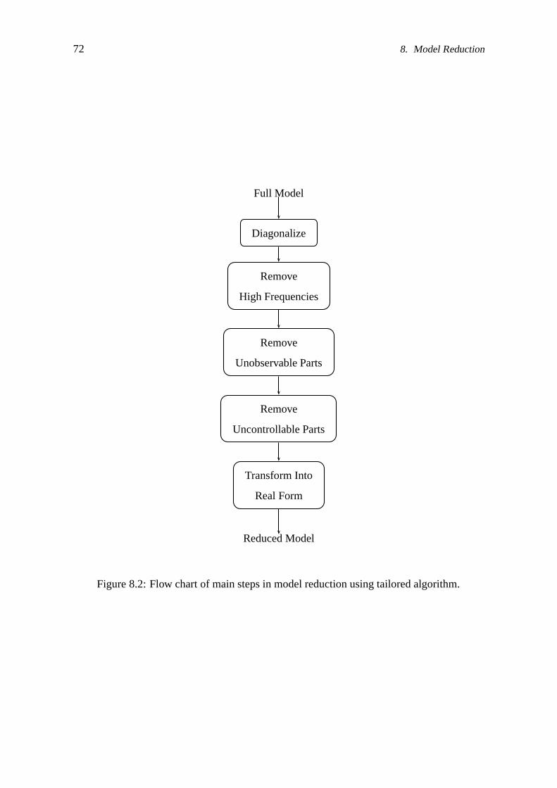
72 8. Model Reduction
Full Model
Diagonalize
Remove
High Frequencies
Remove
Unobservable Parts
Remove
Uncontrollable Parts
Transform Into
Real Form
Reduced Model
Figure 8.2: Flow chart of main steps in model reduction using tailored algorithm.
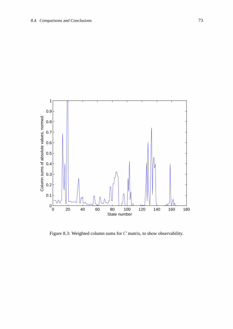
8.4. Comparisons and Conclusions 73
0 20 40 60 80 100 120 140 160 1800
0.1
0.2
0.3
0.4
0.5
0.6
0.7
0.8
0.9
1
State number
Col
umn
sum
s of
abs
olut
e va
lues
, nor
med
.
Figure 8.3: Weighted column sums for C matrix, to show observability.

74 8. Model Reduction
0 20 40 60 80 100 1200
0.1
0.2
0.3
0.4
0.5
0.6
0.7
0.8
0.9
1
State number
Row
sum
s of
abs
olut
e va
lues
, nor
med
.
ActuatorsDisturbances
Figure 8.4: Weighted row sums for B and N matrices, to show controllability from actuatorsand disturbances.

8.4. Comparisons and Conclusions 75
−120
−110
−100
−90
−80
101
−135
−90
−45
0
45
90
135
180
Full modelTailored algorithmFwbredBalred
Mag
nitu
de[d
B]
Frequency [Hz]
Phas
e[d
eg]
Figure 8.5: Model reduction to 21 states. From control input front right, to frequencyweighted acceleration front right.
−180
−160
−140
−120
−100
101
−720
−540
−360
−180
0
Full modelTailored algorithmFwbredBalred
Mag
nitu
de[d
B]
Frequency [Hz]
Phas
e[d
eg]
Figure 8.6: Model reduction to 21 states. From control input front right, to deflection frontright.

76 8. Model Reduction
−105
−100
−95
−90
−85
−80
−75
101
−135
−90
−45
0
45
90
135
180
Full model21 states25 states
Mag
nitu
de[d
B]
Frequency [Hz]
Phas
e[d
eg]
Figure 8.7: Model reduction with and without consideration of disturbances. From controlinput front right, to frequency weighted acceleration front right.
−180
−160
−140
−120
−100
101
−720
−540
−360
−180
0
Full model21 states25 states
Mag
nitu
de[d
B]
Frequency [Hz]
Phas
e[d
eg]
Figure 8.8: Model reduction with and without consideration of disturbances. From controlinput front right, to deflection front right.

8.4. Comparisons and Conclusions 77
−140
−120
−100
−80
−60
−40
101
−720
−540
−360
−180
0
180
Full model21 states25 states
Mag
nitu
de[d
B]
Frequency [Hz]
Phas
e[d
eg]
Figure 8.9: Model reduction with and without consideration of disturbances. From lateraldisturbance at the front wheelset, to frequency weighted acceleration front right.
−100
−80
−60
−40
−20
0
101
−540
−360
−180
0
180
Full model21 states25 states
Mag
nitu
de[d
B]
Frequency [Hz]
Phas
e[d
eg]
Figure 8.10: Model reduction with and without consideration of disturbances. From verticaldisturbance at the front wheelset, to frequency weighted acceleration front right.

78 8. Model Reduction
−120
−100
−80
−60
−40
−20
0
101
−900
−720
−540
−360
−180
0
Full model21 states25 states
Mag
nitu
de[d
B]
Frequency [Hz]
Phas
e[d
eg]
Figure 8.11: Model reduction with and without consideration of disturbances. From rolldisturbance at the front wheelset, to frequency weighted acceleration front right.
−105
−100
−95
−90
−85
−80
−75
101
−180
−90
0
90
180
Full modelTailored 21Tailored 15Tailored 9
Mag
nitu
de[d
B]
Frequency [Hz]
Phas
e[d
eg]
Figure 8.12: Different amount of reduction with tailored algorithm. From control input frontright, to frequency weighted acceleration front right. The curves for 9 states and 15 statesare difficult to tell apart.

8.4. Comparisons and Conclusions 79
−170
−160
−150
−140
−130
−120
−110
101
−720
−540
−360
−180
0
Full modelTailored 21Tailored 15Tailored 9
Mag
nitu
de[d
B]
Frequency [Hz]
Phas
e[d
eg]
Figure 8.13: Different amount of reduction with tailored algorithm. From control input frontright, to deflection front right. The curves for 9 states and 15 states are difficult to tell apart.
−105
−100
−95
−90
−85
−80
−75
101
−180
−90
0
90
180
Full modelTailored 21Tailored 15Tailored 9
Mag
nitu
de[d
B]
Frequency [Hz]
Phas
e[d
eg]
Figure 8.14: Different amount of reduction with tailored algorithm. From control input rearright, to frequency weighted acceleration rear right.

80 8. Model Reduction
−200
−180
−160
−140
−120
−100
101
−270
−180
−90
0
90
Full modelTailored 21Tailored 15Tailored 9
Mag
nitu
de[d
B]
Frequency [Hz]
Phas
e[d
eg]
Figure 8.15: Different amount of reduction with tailored algorithm. From control input rearright, to deflection rear right.

chapter ix
linear quadratic (lq) control design
Linear quadratic (LQ) control is a control method that is using state feedback, and that can beused for multiple-input multiple-output (MIMO) systems. Some aspects of linear quadraticcontrol have been studied on a reduced, stable, linear model from Chapter 8, using Mat-lab/Simulink. Of the reduces models, the one with 9 states has been chosen. All states of themodel are assumed to be measurable. This design model is controllable and observable. Allsimulations and evaluations are made on the reduced model. This is an initial approach tosimplify control design. The system is studied in continues time.
9.1 Background Theory
The following notations are used where nothing else is stated:
x = Ax + Bu (9.1)
y = Cx + Du, (9.2)
where x represents the states, u the control inputs, and y the measured outputs.
9.1.1 Detectability and Stabilizability
A system is stabilizable if there exists a matrix L, such that A−BL is stable. It is detectableif there exists a matrix K, such that A − KC is stable, (Glad and Ljung 2000).
9.1.2 Linear Quadratic Control
Linear quadratic optimization is used to find a linear, causal feedback law that minimizes thecriterion
V = ‖z‖2Q1
+ ‖u‖2Q2
, (9.3)
for a positive definite matrix Q2 and a positive semi-definite matrix Q1. (It is also possibleto have a cross term in the criterion.) z is the controlled variable, and u is the controlsignal. This is solved with the algebraic Riccati Equation. For more details, see (Gladand Ljung 2000). The evaluation criterion can also be chosen as
V =
∫(xT (t)Q1x(t) + u(t)T Q2u(t))dt. (9.4)

82 9. Linear Quadratic (LQ) Control Design
Let Q1 = SST . Then, for the infinite-time, time-invariant problem, there exists a stableclosed-loop optimal system with finite performance index V , if and only if (A, B) is stabi-lizable and (A, S) is detectable, (Anderson and Moore 1989).
LQ and Matlab
Matlab has 2 different build-in commands to calculate a controller by linear quadratic meth-ods (plus some for state estimation), (The MathWorks 2007). Those are:
• lqrFor a continuous-time state-space model, lqr calculates the optimal gain matrix L,such that the state-feedback law u = −Lx minimizes the cost function
V (L) =
∫(xT (t)Qx(t) + u(t)T Ru(t))dt + 2xT (t)Nu(t))dt. (9.5)
It is sufficient to provide the A and B matrices of the state-space model. Of coursealso the penalty weighting matrices Q, R, and N has to be provided.
• lqrylqry is similar to lqr, but uses output weighting. In this case it is necessary toprovide the state-space matrices A, B, C, and D. In this case cost function is
V (L) =
∫(yT (t)Qy(t) + u(t)T Ru(t))dt + 2yT (t)Nu(t))dt. (9.6)
9.1.3 State Observer
LQ control uses state feedback. If not all states are measurable, there is a need to estimatethe states. There are techniques to do this using measured outputs and known (measured)inputs. The states are normally estimated by a so called observer, (Glad and Ljung 2000).Under some conditions, described in (Glad and Ljung 2000), the optimal observer, whichminimizes the error in the estimation, is the Kalman filter. Among other things, the noise isassumed to be white, (Glad and Ljung 2000).
9.2 Inputs and Outputs
This section describes the disturbances that has been chosen to excite the system, as well asthe evaluation of the control.
9.2.1 Disturbances (Inputs)
For simplifying reasons, disturbances have been used only in the vertical direction. Thedisturbances are based on those described in Section 4.1. However, as can be seen in thatsame chapter, disturbance inputs are position, velocity, and acceleration. The data is onlygiven for position. The simulation program Simpack, which the original model is modeledin, calculates velocity and acceleration disturbances from position measurements, using par-tial differential equations. Those have been exported and used also for the simulations inMatlab/Simulink.
9.3. Control 83
The disturbances are given as track disturbances. When simulating the model thereare disturbance inputs at each wheelset. Those are obviously not in the same position onthe track. Therefore, the disturbances have been entered directly in the first wheelset, butdelayed with the times it takes to traverse the distances between the first wheelset and eachof the following. A velocity of 72 km/h has been used. With this velocity, the inputs sufficefor simulating 12.5 seconds.
9.2.2 Evaluation (Outputs)
The outputs from the model are car body acceleration, and deflection between car body andbogie, see Section 4.1. The accelerations have been used to calculate comfort according toSection 2.3. For the deflection, the maximum of the absolute value has been used, to designthe control to keep the bodies within the allowed space. For comparison, all those evaluationparameters have been calculated also for a passive simulation of the same reduced systemwith the same disturbances. Then, the quotient between the active and the passive system hasbeen calculated. If all those quotients are smaller than 1, the performance has been improvedby the control. The maximum of the absolute values of the control signal is also studied, tomake sure it is within reason.
In addition to the variables interesting for control (above), the criterion V (L) is calcu-lated, see Section 9.1. The purpose is to see that the optimization works. V (L) has beencalculated over the simulation time, and integrated numerically using the trapezoid method.
Note that the criterion minimized by linear quadratic control, and the criteria that aredesired, are not the same. However, they have in common that they want the error to besmall.
9.3 Control
The overall method used to find a control law has been to combine output weighting withthe selection of penalty weighting matrices for linear quadratic control. All states have beenmeasured. Therefore, no observer has been used.
Since the model (process) is stable, it is fulfilling the requirements on detectability andstabilizability in Section 9.1. If the weighting matrices are chosen according to Section 9.1,an LQ controller is expected to be found. It will however be seen that it is not quite thatsimple to find a satisfactory control law for this application.
9.3.1 Outputs as Criterion Based on State Space Matrices
If the size of the control signals are not considered of major importance, as long as theydon’t grow towards infinity, it would be a natural approach to concentrate on the outputs inthe criterion to be minimized. Since there is a direct term between the control and the output,and all control signals are used for this, there are some penalty on the control signal anyway.
If the criterion to be minimized by LQ is chosen as
V (L) =
∫ ∞
0
yT (t)y(t)dt, (9.7)

84 9. Linear Quadratic (LQ) Control Design
then, with
y(t) = Cx(t) + Du(t) (9.8)
we get
V (L) =
∫ ∞
0
(Cx(t) + Du(t))T (Cx(t) + Du(t))dt. (9.9)
This can be rewritten as
V (L) =
∫ ∞
0
(xT (t)CT Cx(t) + 2xT (t)CT Du(t) + u(t)T DT Du(t))dt. (9.10)
Unfortunately, the rank of DT D is only 3, although it is a 4 × 4 matrix. Thus, thepenalty weighing function that is wished to be used with u(t)Tu(t), is not positive definite,and therefore this criterion cannot be used. Two approaches, described below, have beenstudied to compensate for this.
Removal of One Control Input
Physical insight has led to the idea to remove one control input. The motivation is as follows:The car body is modeled as a rigid body. Originally, there are 4 force inputs in the verticaldirection. Those control the motions of the car body in the vertical, pitch, and roll directions.That is only 3 directions, which are controlled with 4 inputs. The fourth direction that theinputs is attempting to control, is flexing the car body by for instance pushing the frontleft and rear right corners upwards, while at the same time pulling the front right and rearleft corners downwards. Since the car body is modeled without flexibility here, this is notpossible. There are possibilities to affect the bogies though, since the front and rear bogieare separate.
The control input has been removed by removal of the corresponding parts in the statespace models. What is left is a model with 3 control signals and 8 outputs.
Adding Penalty on Control Input
Another approach is to keep all 4 control signals, but to add a small penalty on them bymodifying Equation 9.7 into
V (L) =
∫ ∞
0
(yT (t)y(t) + δuT (t)u(t))dt, (9.11)
Weighing of Outputs
The outputs are of different size orders. To make the outputs equally important during thecontrol design, which uses either the criterion in Equation 9.7 or in Equation 9.12, the modelhas been modified prior to the control design. If the output of the process is the vector yp,then the output of the design model can be written y = Wyp, where W is a weighing matrix.W has been chosen as a diagonal matrix, which means that each output can be written asyi = wiiypi.
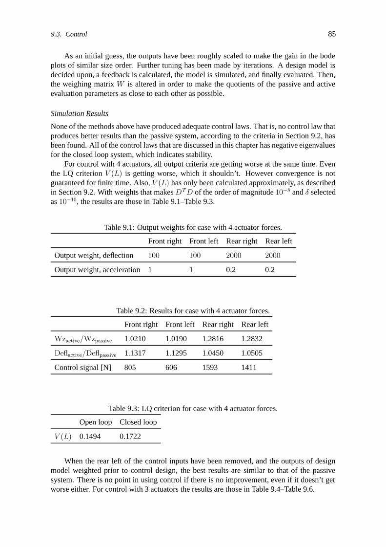
9.3. Control 85
As an initial guess, the outputs have been roughly scaled to make the gain in the bodeplots of similar size order. Further tuning has been made by iterations. A design model isdecided upon, a feedback is calculated, the model is simulated, and finally evaluated. Then,the weighing matrix W is altered in order to make the quotients of the passive and activeevaluation parameters as close to each other as possible.
Simulation Results
None of the methods above have produced adequate control laws. That is, no control law thatproduces better results than the passive system, according to the criteria in Section 9.2, hasbeen found. All of the control laws that are discussed in this chapter has negative eigenvaluesfor the closed loop system, which indicates stability.
For control with 4 actuators, all output criteria are getting worse at the same time. Eventhe LQ criterion V (L) is getting worse, which it shouldn’t. However convergence is notguaranteed for finite time. Also, V (L) has only been calculated approximately, as describedin Section 9.2. With weights that makes DT D of the order of magnitude 10−8 and δ selectedas 10−10, the results are those in Table 9.1–Table 9.3.
Table 9.1: Output weights for case with 4 actuator forces.
Front right Front left Rear right Rear left
Output weight, deflection 100 100 2000 2000
Output weight, acceleration 1 1 0.2 0.2
Table 9.2: Results for case with 4 actuator forces.
Front right Front left Rear right Rear left
Wzactive/Wzpassive 1.0210 1.0190 1.2816 1.2832
Deflactive/Deflpassive 1.1317 1.1295 1.0450 1.0505
Control signal [N] 805 606 1593 1411
Table 9.3: LQ criterion for case with 4 actuator forces.
Open loop Closed loop
V (L) 0.1494 0.1722
When the rear left of the control inputs have been removed, and the outputs of designmodel weighted prior to control design, the best results are similar to that of the passivesystem. There is no point in using control if there is no improvement, even if it doesn’t getworse either. For control with 3 actuators the results are those in Table 9.4–Table 9.6.

86 9. Linear Quadratic (LQ) Control Design
Table 9.4: Output weights for case with 3 actuator forces.
Front right Front left Rear right Rear left
Output weight, deflection 200 200 1700 1700
Output weight, acceleration 0.7 0.8 0.3 0.3
Table 9.5: Results for case with 3 actuator forces.
Front right Front left Rear right Rear left
Wzactive/Wzpassive 1.0221 0.9940 0.9998 0.9728
Deflactive/Deflpassive 1.0095 1.0028 1.0086 1.0098
Control signal [N] 420 770 634 0
9.3.2 Altering Output Penalty
Further studies have been made with other penalties. A diagonal weighing matrix has beenadded as follows:
V (L) =
∫ ∞
0
(yT (t)Qy(t) + δuT (t)u(t))dt, (9.12)
which can also be written
V (L) =
∫ ∞
0
(xT (t)CT QCx(t) + 2xT (t)CT QDu(t) + u(t)T (DT QD + δI)u(t))dt,
(9.13)
since Q is diagonal, and thus Q = QT . In practice though, the Matlab command lqry,described in Section 9.1, has been used in an attempt to find an adequate controller. Thepenalty weighing matrices Q and R have been chosen as diagonal, and N as 0. That is, nocross terms have been considered. For the design, a combination of scaling of the modelprior to the design, as in Section 9.3.1, and the penalties Q and R, has been used. The modelwas scaled roughly to avoid numerical difficulties, then Q and R was used for tuning. Theoutputs and control signals were studied. Large penalties have been used where the output (orcontrol signal) were too big, and small where there were room for improvement. However,despite extensive searches, no adequate controller was found. There were problems with thatafter a while further increases of the penalties did not change the controller.
9.3.3 LQ With Optimal Feed Forward
The wheelsets will be affected by the the same disturbances, with a time delay. If the distur-bances can be measured, there might be a possibility to compensate for them be use of feedforward. A simple way to estimate if this could lead to a satisfactory design, is to simply setall disturbances at all but the first wheelset to 0. This corresponds to perfect feed forward.

9.4. Concluding Remarks 87
Table 9.6: LQ criterion for case with 3 actuator forces.
Open loop Closed loop
V (L) 0.0700 0.0652
Although is not reasonable to assume this can be implemented, it can be assumed that noth-ing better can be achieved. If disconnecting disturbances does not give a satisfactory result,there is no use trying feed forward.
With the same output weighing as with 3 actuators without feed forward, see Table 9.4,the results in Table 9.7–Table 9.8 are obtained. The control signals are not included, sincepart of the control has been faked. Here both comfort and deflection were improved. If
Table 9.7: Results for case with 3 actuator forces and feed forward.
Front right Front left Rear right Rear left
Wzactive/Wzpassive 0.8316 0.8030 0.8124 0.8132
Deflactive/Deflpassive 0.6250 0.6111 0.4886 0.4903
Table 9.8: LQ criterion for case with 3 actuator forces and feed forward.
Open loop Closed loop
V (L) 0.0705 0.0194
the output weights are changed to keep deflection at today’s level, there is room to improvecomfort further, see Table 9.9–Table 9.11.
9.4 Concluding Remarks
LQ design have proved complicated for this model. Either more thorough studies have tobe made, or a different design method need to be chosen. No satisfactory control have beenfound, even disregarding the size of the control signals. Although the LQ criterion is usuallymade smaller by using control, it is not sufficient to make the output errors smaller by thedesired criteria. It is possible to make some of the criteria smaller, but no controller has beenfound that makes all criteria smaller at the same time, when using the measured disturbances.
If an optimal feed forward could be constructed, there seem to be some possibilities toimprove comfort and decrease deflection. But although this looks promising, it is importantto keep in mind that this is a theoretical upper bound, that in practice might be difficult toeven get close. One major challenge in reality is to measure or estimate the disturbancesduring the ride. Another challenge is to approximate the feed forward design. It would

88 9. Linear Quadratic (LQ) Control Design
Table 9.9: Output weights for case with 3 actuator forces and feed forward, optimized forcomfort.
Front right Front left Rear right Rear left
Output weight, deflection 10 10 100 100
Output weight, acceleration 0.7 0.8 0.3 0.3
Table 9.10: Results for case with 3 actuator forces and feed forward, optimized for comfort.
Front right Front left Rear right Rear left
Wzactive/Wzpassive 0.3214 0.3760 0.5024 0.5077
Deflactive/Deflpassive 0.7492 0.7465 0.9440 0.9467
include an approximate plant inversion, as well as model reduction. Still, this idea could beinteresting for future research.
Another approach could be to try design on another reduced model. However, smallermodels will be less accurate and thus a control designed on those are less likely to workon the original model. Larger models, on the other hand, are prone to cause problems withsimulations and numerics. Also, although all reduced models are designed to be controllableand observable, somewhat larger models are not considered controllable or observable byMatlab. For larger models the simulation times are significantly increased.
It is not reasonable to assume that all states can be measured in reality, as done here.Therefore, an observer will be needed. All states have been measured during simulations toisolate the control problem from the state estimation problem. Before implementation, thecontrol law with state estimator needs to be verified on the original model. However, firsta controller that works sufficiently well on the design model, with known states, has to befound.

9.4. Concluding Remarks 89
Table 9.11: LQ criterion for case with 3 actuator forces and feed forward, optimized forcomfort.
Open loop Closed loop
V (L) 0.0118 1.1077 · 10−4


chapter x
concluding remarks
Concluding remarks can be found in the end of Chapter 5–Chapter 9. In this chapter, asummary of those can be found, along with more general comments and recommendations.
Although it would be challenging for the actuators, it is reasonable to design a verticalactive suspension, when adding the actuators in parallel with passive springs. The modelat hand is not adequate for linear studies of motion sickness. Comfort studies, on the otherhand, could be feasible. However, there are nonlinearities, and those are more pronouncedat higher frequencies, which makes the linear model less reliable for high frequencies.
The coupling between the different inputs and outputs are high. Also, to decouple thesystem to make single-input single-output (SISO) control possible, does not look promising.It is not surprising that there are problems with coupling. The car body is stiff, and thecorners cannot be controlled independently. Also, the number of inputs is lower than thenumber of outputs, which means some outputs could not be used. To make multiple-inputmultiple-output (MIMO) design possible, model reduction is needed. The model can bereduced in different ways, to different extents. Which models that are sufficient for controldesign cannot be know until a control design is found and is tested on the original model.However, if a too big model is chosen for control design, there are numerical issues. Linearquadratic control have been attempted with no success. A problem is that the LQ criterion isnot the same as the criteria used in this thesis.
Generally, the problem is numerically challenging, which should be kept in mind.
10.1 Future Work
There are room for further improvements in each of the areas studied. However, it is notnecessarily refining those techniques that will lead to a satisfactory active suspension. A listof suggested things to study follows here.
• Study the model with more simplified assumptions, such as symmetry of vehicle and /or disturbances.
• Improve model simplification, for instance by combining different techniques.
• Generate a model by physical modeling or system identification, instead of by usingmodel reduction.
• An attempt could be made on designing the control on a model using flexible bodies.That would mitigate the problem that there are more control inputs than there are

92 10. Concluding Remarks
degrees of freedom that can be controlled in the car body. On the other hand thiswould make the model even more complicated.
• Change the positions of the actuators. Also, the number of actuators used can bereconsidered.
• Improve control design.
• Evaluate the control design on the original model.
• Model actuator dynamics.
• Calculate forces from passive components that are wished to be removed, and includethem in the control law. This could also be done without adding any further control.
• Model measurement noise.

appendices


appendix a
passenger model
When simulations are run with full load, passengers are modeled as masses, springs, anddampers, according to ISO 5982-1981 (E), (Mechanical vibration and shock - Vibration andshock – Mechanical driving point impedance of the human body 1981). The ISO-standarddescribes how to model a seated or standing person in the vertical direction with two masses,two springs, and two dampers, each. The seated and standing human is not modeled in thesame way. The standard also includes information about a human in supine position, butthere are no people laying down in this model, so that is not used here. To model the lateraldirection, the spring and damper values from the ISO-standard have been divided by two.The choice of model for the lateral direction is rather random. Different ways to model thelateral direction will alter the simulation results, but not severely, according to simulations.Since the car body of the vehicle is modeled as rigid instead of flexible, there will be errorsanyway, and to model the passengers very well is therefore not motivated. The humans aremodeled with only translational degrees of freedom, and the I-tensors of the masses havebeen neglected. In order to reduce the amount of modeling, the humans have been lumpedtogether in six lumps: four with seated people and two with standing. The placements in thecar body are as follows: In the longitudinal direction, the length of the car body was reducedby 10%, and the remaining length was divided by 4. An equal amount of both standing andsitting people were then placed at that distance from the center in both directions. In thelateral direction, all standing people were placed in the middle. For the seated people, themaximum width of the car body was divided by 4. The seated people was then placed thatdistance away from the center, in both directions. See Figure 1.
−15 −10 −5 0 5 10 15
−2
0
2
[meter]
[met
er]
Figure 1: Placement of passengers. x denotes sitting and o denotes standing passengers.
In the vertical direction, the standing passengers are connected to the floor, with centerof gravity 1.00 m above the floor. The sitting passengers have been connected to a point0.45 m above the floor, with center of gravity 0.20 m above the point of connection. Thereare 100 seated people in the model, each weighing 75 kg. Then there are 43.68 standing

96 A. Passenger Model
people. The weight of one passenger is according to ISO 5982-1981 (E), which is not thesame weight as Bombardier uses for one passenger. The number of standing passengers havehowever been increased to reach the same total payload.

appendix b
disturbance dynamics modeling by stateexpansion
There are dynamic dependencies between the disturbances from the rail. The disturbanceinputs are acceleration, velocity, and position displacements of the rail, as experienced bythe moving railway vehicle. When sending disturbances into the model, those dynamic de-pendencies must be taken into account, for the disturbances to be physically correct. Thosedependencies can, however, also be incorporated in the model. Starting from the acceler-ation, it is possible to calculate the velocity and positions by integrations. (Assuming thestarting point is at rest.) Such a modeling will reduce the number of disturbance inputs, butalso leads to more states. The modeling to incorporate the disturbance dynamics into themodel is described in this appendix.
Assume the original model is expressed with the state space model
xo = Aoxo + Bou + Nowo (B.1)
y = Coxo + Dou + Mowo, (B.2)
where xo are the original states, wo are the original disturbances, and the outputs y andcontrol inputs u will stay the same before and after incorporating the disturbance dynamicsinto the model.
Let the number of original states be J , and the number of original disturbances K, ofwhich there are K/3 each of positions, velocities, and accelerations. Then Equation B.1–Equation B.2 can be written as
xo = Aoxo + Bou +(No,1 No,2 No,3 · · · No,K
)
⎛⎜⎜⎜⎜⎜⎜⎜⎜⎜⎝
wo,1
wo,2
wo,3
...
wo,K
⎞⎟⎟⎟⎟⎟⎟⎟⎟⎟⎠
(B.3)
y = Coxo + Dou +(Mo,1 Mo,2 Mo,3 · · · Mo,K
)
⎛⎜⎜⎜⎜⎜⎜⎜⎜⎜⎝
wo,1
wo,2
wo,3
...
wo,K
⎞⎟⎟⎟⎟⎟⎟⎟⎟⎟⎠
. (B.4)

98 B. Disturbance Dynamics Modeling by State Expansion
Let the input order of the disturbances be first position, then velocity, then acceleration,repeated for each physical disturbance. Then wo2 = wo,1, wo,3 = wo,2 = wo,1, wo,5 = wo,4,wo,6 = wo,5 = wo,4, etc. Add new states as
xJ+1 = wo,1
xJ+2 = wo,2
xJ+3 = wo,4
xJ+4 = wo,5
...
xJ+2K/3 = wo,K−1
(B.5)
Now, the state vector can be written as
x =
⎛⎜⎜⎜⎜⎜⎜⎜⎜⎜⎜⎜⎜⎜⎜⎜⎝
xo
xJ+1
xJ+2
xJ+3
xJ+4
...
xJ+2K/3
⎞⎟⎟⎟⎟⎟⎟⎟⎟⎟⎟⎟⎟⎟⎟⎟⎠
. (B.6)
The remaining disturbances will be kept as disturbance inputs for the modified system. Thedisturbances for the modified system can now be written as
w =
⎛⎜⎜⎜⎜⎜⎜⎝
w1
w2
...
wK/3
⎞⎟⎟⎟⎟⎟⎟⎠
=
⎛⎜⎜⎜⎜⎜⎜⎝
wo,3
wo,6
...
wo,K
⎞⎟⎟⎟⎟⎟⎟⎠
. (B.7)
The derivatives of the new states can now be expressed in other states and disturbance inputsas
xJ+1 = xJ+2
xJ+2 = w1
xJ+3 = xJ+4 (B.8)
xJ+4 = w2
...
xJ+2K/3 = w2

99
Now, the full new model can be written as
x = Ax + Bu + Nw (B.9)
y = Cx + Du + Mw, (B.10)
where
A =
⎛⎜⎜⎜⎜⎜⎜⎜⎜⎜⎜⎜⎜⎜⎜⎜⎜⎜⎜⎜⎜⎜⎜⎝
Ao No,1 No,2 No,4 No,5 · · · No,K−2 No,K−1
0 0 1 0 0 · · · 0 0
0 0 0 0 0 · · · 0 0
0 0 0 0 1 · · · 0 0
0 0 0 0 0 · · · 0 0
......
......
.... . .
......
0 0 0 0 0 · · · 0 1
0 0 0 0 0 · · · 0 0
⎞⎟⎟⎟⎟⎟⎟⎟⎟⎟⎟⎟⎟⎟⎟⎟⎟⎟⎟⎟⎟⎟⎟⎠
, (B.11)
B =
⎛⎜⎜⎜⎜⎜⎜⎜⎜⎜⎝
Bo
0
0...
0
⎞⎟⎟⎟⎟⎟⎟⎟⎟⎟⎠
, (B.12)
N =
⎛⎜⎜⎜⎜⎜⎜⎜⎜⎜⎜⎜⎜⎜⎜⎜⎜⎜⎜⎜⎜⎜⎜⎝
No,3 No,6 · · · No,K
0 0 · · · 0
1 0 · · · 0
0 0 · · · 0
0 1 · · · 0
......
. . ....
0 0 · · · 0
0 0 · · · 1
⎞⎟⎟⎟⎟⎟⎟⎟⎟⎟⎟⎟⎟⎟⎟⎟⎟⎟⎟⎟⎟⎟⎟⎠
, (B.13)
C =(
Co Mo,1 Mo,2 Mo,4 Mo,5 · · · Mo,K−2 Mo,K−1
), (B.14)
D =(Do 0 0 · · · 0
), (B.15)

and
M =(
Mo,3 Mo,6 · · · Mo,K
). (B.16)

appendix c
single transfer function derived from adiagonal mimo system
For a system represented on state space form,
x = Ax + Bu (C.1)
y = Cx + Du, (C.2)
the transfer functions can be written as
G(s) = C(sI − A)−1B + D, (C.3)
where I is the identity matrix, (Glad and Ljung 1989).If A is diagonal, so is (sI − A). Therefore, block inversion can be used, with each
element on the diagonal being a block of size 1 × 1, (Rade and Westergren 1998). With Nstates we get:
(sI − A)−1 =
⎛⎜⎜⎜⎜⎜⎜⎝
1s−a11
0
1s−a22
. . .
0 1s−aNN
⎞⎟⎟⎟⎟⎟⎟⎠
. (C.4)
Inserting Equation C.4 into Equation C.3 yields, with J number of inputs and K numberof outputs:

G(s) =
⎛⎜⎜⎜⎝
c11 · · · c1N
.... . .
...
cK1 · · · cKN
⎞⎟⎟⎟⎠
⎛⎜⎜⎜⎝
1s−a11
0. . .
0 1s−aNN
⎞⎟⎟⎟⎠
⎛⎜⎜⎜⎝
b11 · · · b1J
.... . .
...
bN1 · · · bNJ
⎞⎟⎟⎟⎠ + D(s) = (C.5)
=
⎛⎜⎜⎜⎜⎜⎜⎝
c11s−a11
c12s−a22
· · · c1N
s−aNN
c21s−a11
c22s−a22
· · · c2N
s−aNN
......
. . ....
cK1
s−a11
cK2
s−a22· · · cKN
s−aNN
⎞⎟⎟⎟⎟⎟⎟⎠
⎛⎜⎜⎜⎝
b11 · · · b1J
.... . .
...
bN1 · · · bNJ
⎞⎟⎟⎟⎠ + D(s) = (C.6)
=
⎛⎜⎜⎜⎝
∑Nn=1
c1nbn1
s−ann· · · ∑N
n=1c1nbnJ
s−ann
.... . .
...∑Nn=1
cKnbn1
s−ann· · · ∑N
n=1cKnbnJ
s−ann
⎞⎟⎟⎟⎠ + D(s). (C.7)
Thus, the transfer function from input number j to output number k can be written:
gkj =N∑
n=1
cknbnj
s − ann
+ dkj. (C.8)

appendix d
numerical results from feasibility chapter
Here, the full numerical results from the feasibility studies in Chapter 5, are listed. The casesare defined in Section 5.3.1. In the following tables the parts of the variables stands for:
F Force
P Power
Wz Comfort number (Wz)
Z Vertical deflection (between car body and bogie)
Al Roll angle α (between car body and bogie)
ARB Anti-roll bar
VD Vertical damper
B1 Bogie 1
B2 Bogie 2
R Right
L Left
C Center
x Longitudinal
y Lateral
z Vertical
D.1 Forces in Anti-Roll Bar and Damper
The following table shows the mean and maximum forces in the anti-roll bar and damper,separately. The mean is the mean value taken on the absolute value,
F mean =1
N
N∑i=1
|Fi|.

104 D. Numerical Results from Feasibility Chapter
Case 1 Case 2 Case 3 Case 4 Case 5
F mean ARB B1 R [kN] 5.0467 23.002 32.009 6.2134 7.6153
F max ARB B1 R [kN] 29.329 31.359 40.662 24.165 26.852
F mean ARB B1 L [kN] 5.0463 23.013 32.024 6.2136 7.6148
F max ARB B1 L [kN] 29.336 31.338 40.749 23.953 26.883
F mean ARB B2 R [kN] 4.0703 22.941 31.898 5.8434 7.5232
F max ARB B2 R [kN] 20.832 33.092 41.204 21.158 24.067
F mean ARB B2 L [kN] 4.0667 22.962 31.929 5.8408 7.5227
F max ARB B2 L [kN] 20.861 33.166 41.211 21.172 24.063
F mean VD B1 R [kN] 0.6280 0.3610 0.3577 0.4107 0.4065
F max VD B1 R [kN] 6.1157 2.1355 2.1413 3.9358 3.1779
F mean VD B1 L [kN] 0.6279 0.3661 0.3632 0.4119 0.4108
F max VD B1 L [kN] 5.7143 1.7129 1.6909 3.6121 3.8905
F mean VD B2 R [kN] 0.6268 0.3504 0.3406 0.4275 0.4391
F max VD B2 R [kN] 4.7412 2.0226 2.2793 3.1899 3.5197
F mean VD B2 L [kN] 0.6187 0.3559 0.3412 0.4283 0.4379
F max VD B2 L [kN] 5.2267 1.8157 1.6817 2.8551 2.9135
The following table shows the sum of the forces in the anti-roll bar and damper. Theforces are added with sign. The total forces are evaluated in each time sample, before calcu-lating mean and maximum forces.
Case 1 Case 2 Case 3 Case 4 Case 5
F mean B1 R [kN] 5.0988 23.002 32.008 6.2315 7.6347
F max B1 R [kN] 28.378 32.035 41.232 25.025 27.198
F mean B1 L [kN] 5.0990 23.013 32.025 6.2309 7.6325
F max B1 L [kN] 27.897 31.330 40.717 24.894 26.955
F mean B2 R [kN] 4.1173 22.940 31.897 5.8655 7.5468
F max B2 R [kN] 21.333 33.407 41.605 21.524 26.484
F mean B2 L [kN] 4.1125 22.961 31.928 5.8620 7.5453
F max B2 L [kN] 21.072 33.161 41.291 21.227 26.341

D.2. Ideal Power Dissipation in Anti-Roll Bar and Damper 105
D.2 Ideal Power Dissipation in Anti-Roll Bar and Damper
The following table shows the mean and maximum powers in the anti-roll bar and damper,separately.
Case 1 Case 2 Case 3 Case 4 Case 5
P mean ARB B1 R [kW] 0.1843 0.4187 0.5817 0.1352 0.1624
P max ARB B1 R [kW] 4.3051 2.5907 3.6525 3.0065 2.7924
P mean ARB B1 L [kW] 0.1842 0.4583 0.6361 0.1382 0.1649
P max ARB B1 L [kW] 3.5521 3.1055 4.0418 2.4493 2.1020
P mean ARB B2 R [kW] 0.1483 0.4163 0.5628 0.1366 0.1780
P max ARB B2 R [kW] 3.7406 2.3567 3.2387 2.0719 2.7155
P mean ARB B2 L [kW] 0.1494 0.4424 0.5853 0.1362 0.1750
P max ARB B2 L [kW] 4.3637 2.2949 2.8302 1.9171 2.3432
P mean VD B1 R [kW] 0.0362 0.0108 0.0105 0.0152 0.0151
P max VD B1 R [kW] 1.8701 0.2280 0.2293 0.7745 0.5050
P mean VD B1 L [kW] 0.0360 0.0107 0.0105 0.0155 0.0153
P max VD B1 L [kW] 1.6327 0.1467 0.1430 0.6524 0.7568
P mean VD B2 R [kW] 0.0346 0.0102 0.0097 0.0159 0.0168
P max VD B2 R [kW] 1.1240 0.2046 0.2598 0.5088 0.6194
P mean VD B2 L [kW] 0.0342 0.0101 0.0092 0.0160 0.0168
P max VD B2 L [kW] 1.3659 0.1648 0.1414 0.4076 0.4244
The following table shows the sum of the powers in the anti-roll bar and damper.
Case 1 Case 2 Case 3 Case 4 Case 5
P mean B1 R [kW] 0.1838 0.4187 0.5817 0.1357 0.1616
P max B1 R [kW] 3.8135 2.7557 3.7976 2.7751 2.5880
P mean B1 L [kW] 0.1904 0.4585 0.6363 0.1395 0.1671
P max B1 L [kW] 4.0718 3.0722 4.0144 2.5590 2.3745
P mean B2 R [kW] 0.1508 0.4168 0.5632 0.1368 0.1760
P max B2 R [kW] 3.6918 2.3257 3.1737 2.0725 2.5205
P mean B2 L [kW] 0.1549 0.4422 0.5851 0.1389 0.1794
P max B2 L [kW] 4.5930 2.2715 2.7850 2.0006 2.6840
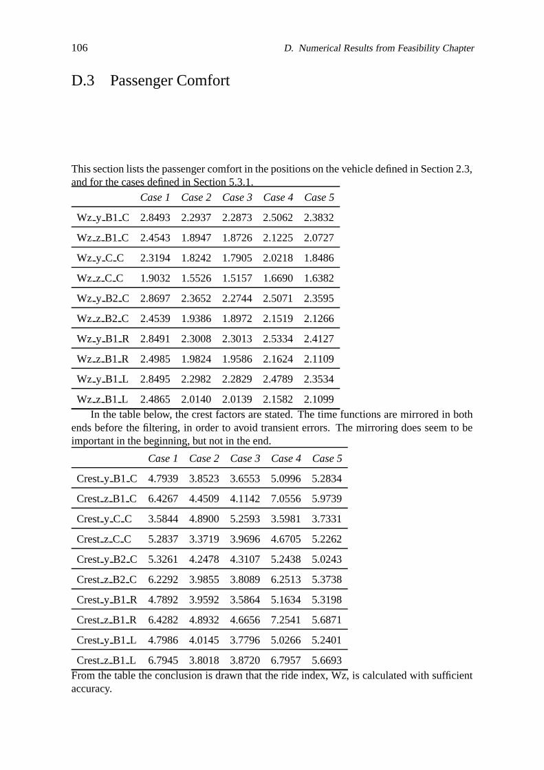
106 D. Numerical Results from Feasibility Chapter
D.3 Passenger Comfort
This section lists the passenger comfort in the positions on the vehicle defined in Section 2.3,and for the cases defined in Section 5.3.1.
Case 1 Case 2 Case 3 Case 4 Case 5
Wz y B1 C 2.8493 2.2937 2.2873 2.5062 2.3832
Wz z B1 C 2.4543 1.8947 1.8726 2.1225 2.0727
Wz y C C 2.3194 1.8242 1.7905 2.0218 1.8486
Wz z C C 1.9032 1.5526 1.5157 1.6690 1.6382
Wz y B2 C 2.8697 2.3652 2.2744 2.5071 2.3595
Wz z B2 C 2.4539 1.9386 1.8972 2.1519 2.1266
Wz y B1 R 2.8491 2.3008 2.3013 2.5334 2.4127
Wz z B1 R 2.4985 1.9824 1.9586 2.1624 2.1109
Wz y B1 L 2.8495 2.2982 2.2829 2.4789 2.3534
Wz z B1 L 2.4865 2.0140 2.0139 2.1582 2.1099In the table below, the crest factors are stated. The time functions are mirrored in both
ends before the filtering, in order to avoid transient errors. The mirroring does seem to beimportant in the beginning, but not in the end.
Case 1 Case 2 Case 3 Case 4 Case 5
Crest y B1 C 4.7939 3.8523 3.6553 5.0996 5.2834
Crest z B1 C 6.4267 4.4509 4.1142 7.0556 5.9739
Crest y C C 3.5844 4.8900 5.2593 3.5981 3.7331
Crest z C C 5.2837 3.3719 3.9696 4.6705 5.2262
Crest y B2 C 5.3261 4.2478 4.3107 5.2438 5.0243
Crest z B2 C 6.2292 3.9855 3.8089 6.2513 5.3738
Crest y B1 R 4.7892 3.9592 3.5864 5.1634 5.3198
Crest z B1 R 6.4282 4.8932 4.6656 7.2541 5.6871
Crest y B1 L 4.7986 4.0145 3.7796 5.0266 5.2401
Crest z B1 L 6.7945 3.8018 3.8720 6.7957 5.6693From the table the conclusion is drawn that the ride index, Wz, is calculated with sufficientaccuracy.
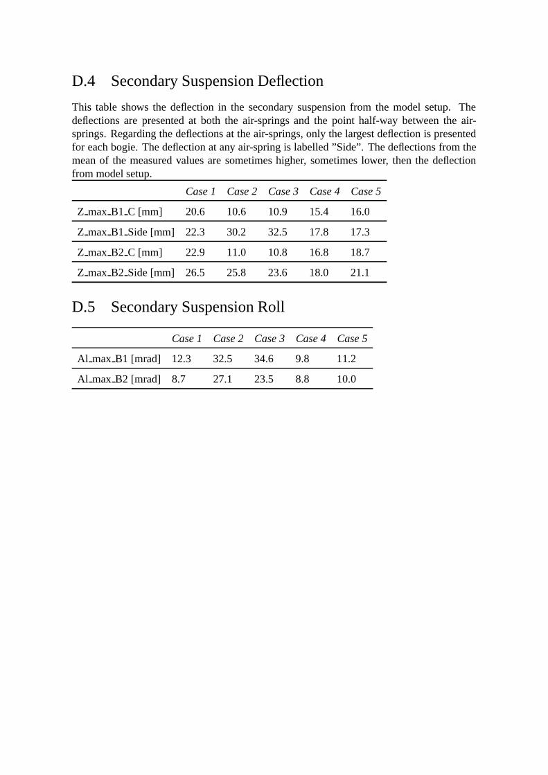
D.4 Secondary Suspension Deflection
This table shows the deflection in the secondary suspension from the model setup. Thedeflections are presented at both the air-springs and the point half-way between the air-springs. Regarding the deflections at the air-springs, only the largest deflection is presentedfor each bogie. The deflection at any air-spring is labelled ”Side”. The deflections from themean of the measured values are sometimes higher, sometimes lower, then the deflectionfrom model setup.
Case 1 Case 2 Case 3 Case 4 Case 5
Z max B1 C [mm] 20.6 10.6 10.9 15.4 16.0
Z max B1 Side [mm] 22.3 30.2 32.5 17.8 17.3
Z max B2 C [mm] 22.9 11.0 10.8 16.8 18.7
Z max B2 Side [mm] 26.5 25.8 23.6 18.0 21.1
D.5 Secondary Suspension Roll
Case 1 Case 2 Case 3 Case 4 Case 5
Al max B1 [mrad] 12.3 32.5 34.6 9.8 11.2
Al max B2 [mrad] 8.7 27.1 23.5 8.8 10.0

108 D. Numerical Results from Feasibility Chapter

references


111
bibliography
Agren, J. (2004–2005). Private communication. Bombardier Transportation.
Anderson, B. and Moore, J. (1989). Optimal control – linear quadratic methods, Prentice-Hall, Englewood Cliffs, NJ, USA.
Andersson, E. and Berg, M. (1999). Jarnvagssystem och sparfordon, Railway Group KTH,Stockholm, Sweden.
Andersson, E., Berg, M. and Stichel, S. (2004). Rail Vehicle Dynamics, Railway GroupKTH, Stockholm, Sweden.
Bengtsson, V. and Weisstein, E. (2008). Diagonalizable matrix.*http://mathworld.wolfram.com/DiagonalizableMatrix.html
Benner, P., Mehrmann, V., Sima, V., Huffel, S. V. and Varga, A. (1998). Slicot — a subroutinelibrary in systems and control theory.*citeseer.ist.psu.edu/benner97slicot.html
Breitholtz, C. (2009). Private communication. Chalmers University of Technology.
Glad, T. and Ljung, L. (1989). Reglerteknik – Grundlaggande teori, Studentlitteratur, Lund,Sweden.
Glad, T. and Ljung, L. (2000). Control Theory – Multivariable and Nonlinear Methods,Studentlitteratur, Lund, Sweden.
Goodall, R. and Mei, T. (2006). Active suspensions, in S. Iwnicki (ed.), Handbook of Rail-way Vehicle Dynamics, pp. 327–357.
Intec GmbH (2003). Simpack training, Educational material.*http://www.simpack.com/
Intec GmbH (2005). SIMDOC 8.704, Intec GmbH, Wessling, Germany.*http://www.simpack.com/
Kjellqvist, P. (2002). Modelling and design of electromechanical actuators for active sus-pension in rail vehicles, PhD thesis, KTH Electrical Machines and Power Electronics,Stockholm, Sweden.
Lennartson, B. (2002). Reglerteknikens grunder, 4:th edn, Studentlitteratur, Lund, Sweden.
Mechanical vibration and shock - Evaluation of human exposure to whole-body vibration –Part 1: General requirements (1997). ISO 2631/1-1997(E).
Mechanical vibration and shock - Vibration and shock – Mechanical driving point impedanceof the human body (1981). ISO 5982-1981(E).

112
Niconet (2005). Slicot Manual, Niconet.*http://www.slicot.org/
Nordling, C. and Osterman, J. (1996). Physics Handbook for Science and Engineering, 5:thedn, Studentlitteratur, Lund, Sweden.
Orlova, A. and Boronenko, Y. (2006). The anatomy of railway vehicle running gear, inS. Iwnicki (ed.), Handbook of Railway Vehicle Dynamics, pp. 39–84.
Rade, L. and Westergren, B. (1998). Mathematics Handbook for Science and Engineering,4:th edn, Studentlitteratur, Lund, Sweden.
Roos, B. (2005). Private communication. Bombardier Transportation.
Sedra, A. and Smith, K. (1998). Microelectronic Circuits, 4:th edn, Oxford University Press.
Shinskey, F. (1996). Process Control Systems – Application, Design, and Tuning, McGraw-Hill.
Skogestad, S. and Postlethwaite, I. (1996). Multivariable Feedback Control – Analysis andDesign, John Wiley & Sons.
The MathWorks (2007). Matlab Manual, The MathWorks.*http://www.mathworks.com/
Varga, A. (2000). Model reduction software in the slicot library.*citeseer.ist.psu.edu/varga00model.html
Zolotas, A., Pearson, J. and Goodall, R. (2006). Modelling requirements for the design ofactive stability control strategies for a high speed bogie, Multibody System Dynamics15: 51–66.