2352020

Berichte zur ErdsystemforschungReports on Earth System Science

Variability of theContemporary Southern Ocean

Carbon Fluxes and Storage

Lydia KepplerHamburg 2020

Hinweis

Die Berichte zur Erdsystemforschung werden vom Max-Planck-Institut für Meteorologie in Hamburg in unregelmäßiger Abfolge heraus-gegeben.

Sie enthalten wissenschaftliche und technische Beiträge, inklusive Dissertationen.

Die Beiträge geben nicht notwendigerweise die Auffassung des Instituts wieder.

Die "Berichte zur Erdsystemforschung" führen die vorherigen Reihen "Reports" und "Examens-arbeiten" weiter.

Anschrift / Address

Max-Planck-Institut für MeteorologieBundesstrasse 5320146 HamburgDeutschland

Tel./Phone: +49 (0)40 4 11 73 - 0Fax: +49 (0)40 4 11 73 - 298

name.surname@mpimet.mpg.dewww.mpimet.mpg.de

Notice

The Reports on Earth System Science are published by the Max Planck Institute for Meteorology in Hamburg. They appear in irregular intervals.

They contain scientific and technical contribu-tions, including Ph. D. theses.

The Reports do not necessarily reflect the opinion of the Institute.

The "Reports on Earth System Science" continue the former "Reports" and "Examensarbeiten" of the Max Planck Institute.

Layout

Bettina Diallo and Norbert P. NoreiksCommunication

Copyright

Photos below: ©MPI-MPhotos on the back from left to right:Christian Klepp, Jochem Marotzke,Christian Klepp, Clotilde Dubois,Christian Klepp, Katsumasa Tanaka

Variability of theContemporary Southern Ocean

Carbon Fluxes and Storage

Lydia KepplerHamburg 2020

Berichte zur Erdsystemforschung / Max-Planck-Institut für Meteorologie 235Reports on Earth System Science / Max Planck Institute for Meteorology 2020

ISSN 1614-1199

Lydia Keppleraus Stuttgart, Deutschland

Max-Planck-Institut für MeteorologieThe International Max Planck Research School on Earth System Modelling(IMPRS-ESM)Bundesstrasse 5320146 Hamburg

Universität HamburgGeowissenschaftenMeteorologisches InstitutBundesstr. 5520146 Hamburg

Tag der Disputation: 16. Juni 2020

Folgende Gutachter empfehlen die Annahme der Dissertation:Dr. Peter LandschützerProf. Dr. Johanna Baehr

Vorsitzender des Promotionsausschusses: Prof. Dr. Dirk Gajewski

Dekan der MIN-Fakultät:Prof. Dr. Heinrich Graener

________________

The figure on the front page depicts dissolved inorganic carbon at the surface ocean (y-axis) as a function of latitude (x-axis) and longitude (color). Although not bursting with useful information, it passes as a piece of modern art. A slightly modified version of this figure won the Clim*Art Contest of the 2019 MPI-M annual retreat.

ii

“Humanity is currently enacting a narrative that nature is ours to abuse and exploitand pollute as we see fit, forgetting that we are a part of it. We are part of the webof life, and when we harm one part of that web, we harm ourselves. We urgentlyneed a new narrative, where instead of hubris we have humility. Instead of rapaciousdestruction we have respect and stewardship. Instead of disconnection, we have deepconnection - to nature, to each other, to ourselves, and to our future.”

Roz Savage

iii

Abstract

Around half of the ocean’s uptake of anthropogenic carbon from theatmosphere currently takes place in the Southern Ocean. However, thevariability of this important carbon sink, as well as the drivers behind thisvariability, are still debated and it is unclear if the Southern Ocean willremain a carbon sink in the future. Until this PhD project, the developmentof the Southern Ocean carbon uptake at the air-sea interface was unknownbased on observations beyond 2011. Furthermore, the seasonal tointerannual variability of dissolved inorganic carbon (DIC) in the interiorSouthern Ocean had not been analyzed based on observations at regionalscale. This dissertation closes these research gaps.

In the first part of my dissertation (Appendix A), I investigate theSouthern Ocean carbon flux and its drivers until 2016 using an updatedobservation-based air-sea carbon flux estimate. After a stagnation period inthe 1990s, and a reinvigoration in the 2000s, I find that the Southern Oceancarbon uptake weakened again since about 2011. My study reveals that theSouthern Annular Mode, the dominant mode of climate variability in thesouthern high latitudes, is not the driver behind this weakening due toopposing effects that cancel each other out. Instead, regional shifts insurface wind velocity modulate the recent evolution of the carbon uptake inthe Southern Ocean. In the second part (Appendix B), I develop a monthlyclimatology of global mapped interior DIC fields using a neural-networkmapping approach. Using this new data product, I describe the seasonalcarbon dynamics at global scale, including the phase and amplitude of thesurface seasonal cycle, how deep seasonal signals are detectable, and Iestimate the net community production. In the third part (Appendix C), Iincrease the temporal resolution of my new data product to resolve monthlyfields from 2004 through 2017. I then re-focus on the Southern Ocean toinvestigate the interannual variability of DIC in the water column anddetermine the potential drivers behind this variability. Using this secondnew data product, I demonstrate that sub-surface DIC is subject tosignificant decadal fluctuations. These fluctuations extend to at least 500 mand could be linked to changes in the Meridional Overturning Circulation.

The methods and the publicly available data products I developedprovide an opportunity for further analysis of the global carbon cycle. Thefindings from my PhD project represent an updated estimate of the carbonuptake and storage in the Southern Ocean and enable an improveddescription of the processes and drivers of variability. This knowledgeforms an essential part of our understanding of the global carbon cycle andcan, therefore, contribute to more accurate climate projections, forming animportant basis for political decisions aimed at reducing carbon emissions.

iv

Zusammenfassung

Im Südpolarmeer findet derzeit etwa die Hälfte der ozeanischen Aufnahmevon anthropogenem Kohlenstoff aus der Atmosphäre statt. Über dieVariabilität dieser wichtigen Kohlenstoffsenke sowie die Einflussfaktorendieser Variabilität wird jedoch debattiert, und es ist unklar, ob dasSüdpolarmeer auch in der Zukunft eine Kohlenstoffsenke bleiben wird. Vordiesem Promotionsprojekt fehlte eine Abschätzung der atmosphärischenKohlenstoffaufnahme des Südpolarmeers basierend auf Beobachtungsdatendie nach 2011 erhoben wurden. Des Weiteren wurde die saisonale undzwischenjährliche Variabilität des gelösten anorganischen Kohlenstoffs(DIC) im tiefen Südpolarmeer bisher noch nicht anhand vonBeobachtungsdaten auf regionaler Ebene analysiert. Diese Dissertationschließt die bestehenden Forschungslücken.

Im ersten Teil meiner Dissertation (Anhang A) untersuche ich dieozeanische Kohlenstoffaufnahme aus der Atmosphäre und derenEinflussfaktoren im Südpolarmeer bis 2016 anhand aktualisierterBeobachtungsdaten, die an der Meeresoberfläche erhoben wurden. Nacheiner Stagnationsphase in den 1990er Jahren und einem Wiedererstarken inden 2000er Jahren, ermittle ich, dass die Kohlenstoffaufnahme imSüdpolarmeer seit ca. 2011 erneut nachgelassen hat. Meine Studie zeigt,dass der Southern Annular Mode, der dominante Modus vonKlimaschwankungen in den südlichen hohen Breitengraden, nicht derEinflussfaktor hinter diesem Abschwächen der Senke ist, da sichgegensätzliche Effekte aufheben. Stattdessen kontrollieren regionaleVerschiebungen der Oberflächenwindgeschwindigkeit die jüngsteEntwicklung der Kohlenstoffsenke im Südpolarmeer. Im zweiten Teil(Anhang B) etabliere ich ein Verfahren, das es erlaubt, mithilfe neuronalerNetzwerke die globale Tiefenverteilung von gelöstem anorganischenKohlenstoff als monatliche Klimatologie abzubilden. Mit diesem neuentwickelten Datenprodukt beschreibe ich die saisonale DIC-Dynamik aufglobaler Ebene. Diese Beschreibung erstreckt sich auf die Phase undAmplitude des saisonalen Zyklus an der Oberfläche und dessenTiefenausdehnung, sowie eine Abschätzung der Nettoproduktion vonorganischem Kohlenstoff durch marine Lebensgemeinschaften. Im drittenTeil (Anhang C) erhöhe ich die zeitliche Auflösung dieses Datenprodukts,um auch die zwischenjährlichen Veränderungen der monatlichenDIC-Felder von 2004 bis Ende 2017 aufzulösen. Für die inhaltlicheInterpretation der neu generierten Datensätze lege ich den Schwerpunkterneut auf das Südpolarmeer, um hier die zwischenjährliche Variabilität desgelösten anorganischen Kohlenstoffs in der Wassersäule zu beschreiben unddie möglichen Einflussfaktoren für diese Variabilität zu bestimmen. Anhanddieses zweiten neuen Datenprodukts zeige ich, dass der gelösteanorganische Kohlenstoff unterhalb der Meeresoberfläche signifikanten

v

dekadischen Schwankungen unterliegt. Diese Schwankungen erstreckensich mindestens über die oberen 500 m der Wassersäule und könnten mitÄnderungen der meridionalen Umwälzzirkulation verbunden sein.

Die von mir entwickelten Methoden und öffentlich zur Verfügunggestellten Datenprodukte eröffnen diverse Möglichkeiten zur weiterenAnalyse des globalen Kohlenstoffkreislaufs. Die Ergebnisse meinesPromotionsprojekts stellen eine aktualisierte Abschätzung derKohlenstoffaufnahme und -speicherung im Südpolarmeer dar undermöglichen eine erheblich verbesserte Beschreibung der beteiligtenProzesse und Einflussfaktoren. Dieses Wissen ist ein wesentlicherBestandteil unseres Verständnisses des globalen Kohlenstoffkreislaufs undkann somit zu genaueren Klimaprojektionen beitragen. Damit bilden dieBefunde auch eine wichtige Grundlage für politische Entscheidungen, dieauf die Reduzierung der Kohlenstoffemissionen abzielen.

vi

Parts of this dissertationpre-published or intendedfor publication

Keppler, L. and P. Landschützer (2019). "Regional Wind VariabilityModulates the Southern Ocean Carbon Sink". In: Scientific Reports 9, 7384.https://doi.org/10.1038/s41598-019-43826-y. Appendix A

Keppler, L., P. Landschützer, N. Gruber, S.K. Lauvset, I. Stemmler (inreview). "Seasonal Carbon Dynamics in the Global Ocean based on aNeural-Network Mapping of Observations". In review at GlobalBiogeochemical Cycles. Appendix B

Keppler, L. and P. Landschützer (in prep.). "Temporary Reduction inSouthern Ocean sub-surface Dissolved Inorganic Carbon". To be submitted toGeophysical Research Letters. Appendix C

vii

Acknowledgments

I have received an incredible amount of support from many people, forwhich I am extremely grateful.

First, I would like to thank my main supervisor. Thank you, PeterLandschützer, for giving me this opportunity, your positive attitude, alwayshaving my back, and everything I learned from you. I also am extremelygrateful for my co-advisors, Jochem Marotzke and Birgit Klein, for theirinvaluable input and support. Many thanks also to Johanna Baehr for herwell-thought-out advice during our panel meetings. I could not have askedfor better support and guidance from my advisory panel throughout myPhD.

I would also like to thank my colleagues and friends from the MPI-M,with special thanks to the Ocean Department, the OAS and DRO groups,the Journal Club and LunchBytes, and the IMPRS. I have been privileged towork with you all and am grateful for the many lessons learned, theinteresting discussions and seminars, as well as the coffee breaks, lunches,Feierabendbiere, and other fun activities. Thank you also for all theadministrative and moral support from Antje, Connie, Michaela, andKornelia.

I am also very grateful for my co-authors—Niki Gruber, Siv Lauvset, andIrene Stemmler. It has been a fantastic experience to write a paper with you.I also want to thank the people that have provided feedback to thisthesis—Laura, Rike, Jens, and Hauke. I am extremely grateful for yourvaluable contributions.

Last but not least, I want to thank my family and friends for their supportand friendship. Our chats and meet-ups have meant a lot to me. Thank youfor the laughs, discussions, and the reminders to focus on self-care. Thankyou, Shupiwe, for your incredible support, moving to Hamburg with me,always believing in me, your editing, and your love. Finally, I want to thankmy grandmother, Oma Evchen. Thank you for all the inspiration, yourremarkable optimism, and your love. I got my passion for the ocean fromyou, and I know how proud you would have been.

viii

Contents

Abstract iii

Zusammenfassung iv

Publications vi

Acknowledgments vii

Lists of Figures and Abbreviations ix

Unifying Essay 11 Background . . . . . . . . . . . . . . . . . . . . . . . . . . . . . . 1

1.1 Basics of the oceanic carbon system . . . . . . . . . . . 11.2 Biogeochemical and physical drivers . . . . . . . . . . 31.3 The relevance of the Southern Ocean . . . . . . . . . . 4

2 Current Knowledge and Research Gaps . . . . . . . . . . . . . . 42.1 Observations of the carbon system in the Southern Ocean . 42.2 The mean Southern Ocean carbon uptake . . . . . . . . 62.3 Southern Ocean carbon uptake variability . . . . . . . . 82.4 Variability in interior Southern Ocean DIC . . . . . . . . 9

3 Machine Learning . . . . . . . . . . . . . . . . . . . . . . . . . . . 103.1 Terminology . . . . . . . . . . . . . . . . . . . . . 103.2 SOM-FFN . . . . . . . . . . . . . . . . . . . . . . 113.3 Approaches developed and used in this study . . . . . . 13

4 Summary of Key Results . . . . . . . . . . . . . . . . . . . . . . . 144.1 Interannual variability of Southern Ocean carbon fluxes . . 144.2 Monthly climatology of global interior DIC . . . . . . . 154.3 Interannual variability of interior Southern Ocean DIC . . 174.4 Drivers of variability at the surface and below . . . . . . 17

5 Outlook and Implications . . . . . . . . . . . . . . . . . . . . . . 18

Appendices 20A Regional Wind Variability Modulates the Southern Ocean

Carbon Sink . . . . . . . . . . . . . . . . . . . . . . . . . . . . . . 21B Seasonal Carbon Dynamics in the Global Ocean based on a

Neural-Network Mapping of Observations . . . . . . . . . . . . 37C Temporary Reduction in Southern Ocean sub-surface

Dissolved Inorganic Carbon . . . . . . . . . . . . . . . . . . . . . 71

Bibliography 86

Declaration of Oath 94

ix

List of Figures

1 Marine Carbon Chemistry . . . . . . . . . . . . . . . . . . . . . 22 Location of recent Southern Ocean carbon measurements . . . 63 Temporal mean Southern Ocean carbon flux . . . . . . . . . . 74 Zonal mean Southern Ocean circulation . . . . . . . . . . . . . 75 Evolution of the Southern Ocean Carbon sink until 2011 . . . 86 Schematic of SOM clustering . . . . . . . . . . . . . . . . . . . 127 Schematic of a generic FFN configuration . . . . . . . . . . . . 138 Extension of the evolution of the Southern Ocean carbon flux 159 Seasonal characteristics of DIC . . . . . . . . . . . . . . . . . . 1610 Change in DIC over time and depth . . . . . . . . . . . . . . . 18A.1 Recent Southern Ocean carbon sink variability . . . . . . . . . 25A.2 The SAM’s effect on the Southern Ocean carbon sink . . . . . 27A.3 Physical sea surface properties and the carbon flux . . . . . . 29A.4 Regional shifts in sea level pressure and surface winds . . . . 32B.1 Ship measurements of DIC . . . . . . . . . . . . . . . . . . . . 41B.2 Spatial distribution of DIC . . . . . . . . . . . . . . . . . . . . . 49B.3 Comparison with Lauvset . . . . . . . . . . . . . . . . . . . . . 50B.4 Comparison with HAMOCC (time-mean) . . . . . . . . . . . . 52B.5 Seasonal cycle in climate regions . . . . . . . . . . . . . . . . . 53B.6 Amplitude and phase of the seasonal cycle . . . . . . . . . . . 54B.7 Regional response function . . . . . . . . . . . . . . . . . . . . 55B.8 Comparison with HAMOCC (seasonal cycle) . . . . . . . . . . 56B.9 Comparison with HOT time-series . . . . . . . . . . . . . . . . 57B.10 Comparison with BATS time-series . . . . . . . . . . . . . . . 58B.11 Comparison with SOCCOM floats . . . . . . . . . . . . . . . . 59B.12 Nodal depth of DIC . . . . . . . . . . . . . . . . . . . . . . . . 60B.13 Spatial distribution of summer NCP . . . . . . . . . . . . . . . 61B_SI.1 Location and variability of SOM clusters . . . . . . . . . . . . 66B_SI.2 Schematic of our FFN configuration . . . . . . . . . . . . . . . 68B_SI.3 Time or location as predictor . . . . . . . . . . . . . . . . . . . 69B_SI.4 Summary of validation tests . . . . . . . . . . . . . . . . . . . . 70C.1 Change in DIC over time and depth . . . . . . . . . . . . . . . 76C.2 Temporal sub-surface reduction in direct DIC measurements . 77C.3 Comparison with independent data . . . . . . . . . . . . . . . 79C.4 Physical drivers of the interior DIC . . . . . . . . . . . . . . . . 81C_SI.1 Time-mean of DIC in the Southern Ocean . . . . . . . . . . . . 84C_SI.2 Timeline of the recent SAM . . . . . . . . . . . . . . . . . . . . 85

x

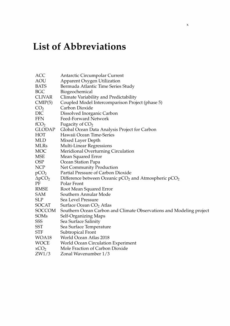
List of Abbreviations

ACC Antarctic Circumpolar CurrentAOU Apparent Oxygen UtilizationBATS Bermuda Atlantic Time Series StudyBGC BiogeochemicalCLIVAR Climate Variability and PredictabilityCMIP(5) Coupled Model Intercomparison Project (phase 5)CO2 Carbon DioxideDIC Dissolved Inorganic CarbonFFN Feed-Forward NetworkfCO2 Fugacity of CO2GLODAP Global Ocean Data Analysis Project for CarbonHOT Hawaii Ocean Time-SeriesMLD Mixed Layer DepthMLRs Multi-Linear RegressionsMOC Meridional Overturning CirculationMSE Mean Squared ErrorOSP Ocean Station PapaNCP Net Community ProductionpCO2 Partial Pressure of Carbon Dioxide∆pCO2 Difference between Oceanic pCO2 and Atmospheric pCO2PF Polar FrontRMSE Root Mean Squared ErrorSAM Southern Annular ModeSLP Sea Level PressureSOCAT Surface Ocean CO2 AtlasSOCCOM Southern Ocean Carbon and Climate Observations and Modeling projectSOMs Self-Organizing MapsSSS Sea Surface SalinitySST Sea Surface TemperatureSTF Subtropical FrontWOA18 World Ocean Atlas 2018WOCE World Ocean Circulation ExperimentxCO2 Mole Fraction of Carbon DioxideZW1/3 Zonal Wavenumber 1/3

1

Unifying Essay

This thesis is structured as a cumulative dissertation, where the UnifyingEssay precedes three Appendices containing the research articles I producedas part of my PhD. The Unifying Essay first introduces my PhD project byproviding the scientific background knowledge and then putting myresearch into the broader literature context, presenting the currentknowledge and related research gaps. After describing some of the methodsI developed and applied during this PhD, I present my main researchfindings and a brief overview of how this study may affect subsequentresearch and the implications of my findings.

1 Background

1.1 Basics of the oceanic carbon system

Of the carbon dioxide (CO2) emitted annually by humans, currently, onlyabout half accumulates in the atmosphere, whereas the land and ocean takeup the rest. Specifically, the Global Carbon Budget (Friedlingstein et al.,2019) estimates, that between 2009 and 2018, the ocean took up 2.5 ±0.6 PgCyr−1 from the atmosphere, which is approximately 23% of the annualanthropogenic emissions for that period (1 PgC = 1 petagram carbon = 1015

grams of carbon). Due to this oceanic uptake of anthropogenic carbon, theocean plays an important mitigating role in climate change (Ciais et al.,2014).

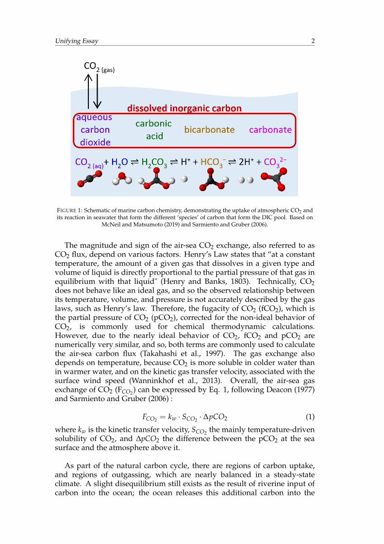
The oceanic uptake of CO2 from the atmosphere occurs at the airsea-interface (Fig. 1). When gaseous CO2 dissolves in the ocean, the nowaqueous CO2 reacts chemically with water molecules (H2O) and formscarbonic acid (H2CO3), which can dissociate twice into bicarbonate ions(HCO3

−) and carbonate ions (CO32−) (Sarmiento and Gruber, 2006; Zeebe

and Wolf-Gladrow, 2001). These ‘species’ of inorganic carbon in seawaterare collectively referred to as dissolved inorganic carbon (DIC). In itsdissolved form, the carbon can be transported through currents andturbulent mixing (Heinze et al., 2015). However, the chemical equilibriumreactions described here, can occur in both directions and so, carbon can betaken up by the ocean and stored as DIC, but DIC can also outgas into theatmosphere.

Unifying Essay 2

FIGURE 1: Schematic of marine carbon chemistry, demonstrating the uptake of atmospheric CO2 andits reaction in seawater that form the different ‘species’ of carbon that form the DIC pool. Based on

McNeil and Matsumoto (2019) and Sarmiento and Gruber (2006).

The magnitude and sign of the air-sea CO2 exchange, also referred to asCO2 flux, depend on various factors. Henry’s Law states that “at a constanttemperature, the amount of a given gas that dissolves in a given type andvolume of liquid is directly proportional to the partial pressure of that gas inequilibrium with that liquid" (Henry and Banks, 1803). Technically, CO2does not behave like an ideal gas, and so the observed relationship betweenits temperature, volume, and pressure is not accurately described by the gaslaws, such as Henry’s law. Therefore, the fugacity of CO2 (fCO2), which isthe partial pressure of CO2 (pCO2), corrected for the non-ideal behavior ofCO2, is commonly used for chemical thermodynamic calculations.However, due to the nearly ideal behavior of CO2, fCO2 and pCO2 arenumerically very similar, and so, both terms are commonly used to calculatethe air-sea carbon flux (Takahashi et al., 1997). The gas exchange alsodepends on temperature, because CO2 is more soluble in colder water thanin warmer water, and on the kinetic gas transfer velocity, associated with thesurface wind speed (Wanninkhof et al., 2013). Overall, the air-sea gasexchange of CO2 (FCO2) can be expressed by Eq. 1, following Deacon (1977)and Sarmiento and Gruber (2006) :

FCO2 = kw · SCO2 · ∆pCO2 (1)

where kw is the kinetic transfer velocity, SCO2 the mainly temperature-drivensolubility of CO2, and ∆pCO2 the difference between the pCO2 at the seasurface and the atmosphere above it.

As part of the natural carbon cycle, there are regions of carbon uptake,and regions of outgassing, which are nearly balanced in a steady-stateclimate. A slight disequilibrium still exists as the result of riverine input ofcarbon into the ocean; the ocean releases this additional carbon into the

Unifying Essay 3

atmosphere (Resplandy et al., 2018). In addition to the natural carbon cycle,the release of anthropogenic CO2 into the atmosphere creates a partialpressure gradient that results in net oceanic uptake of carbon (Ciais et al.,2014).

Compared to the ocean, CO2 in the atmosphere is relatively well-mixed,meaning that the concentration does not vary as much around the globe.However, different factors modulate the oceanic pCO2, resulting in largevariations that are orders of magnitude larger than the variations inatmospheric pCO2. Subsequently, at the regional scale, the sea surface pCO2largely controls the sign and magnitude of the flux (Landschützer et al.,2014). Different physical and biogeochemical processes drive the variabilityin the air-sea carbon flux, and these are superimposed on the positive trendof increased carbon uptake due to the anthropogenic perturbation(Sarmiento and Gruber, 2006; Takahashi et al., 2002).

The positive effect of the oceans abating climate change by absorbinganthropogenic CO2 (Friedlingstein et al., 2019) does not occur withoutnegative side effects: the reaction of CO2 in sea-water releases hydrogenions (H+, Fig. 1), directly lowering the pH of the seawater (Sarmiento andGruber, 2006; Zeebe and Wolf-Gladrow, 2001). Subsequently, additional DICin the ocean lowers its pH, a process called ocean acidification (Doney et al.,2009). In more acidic water, calcifying organisms such as calcareousplankton, corals, and mollusks, struggle to produce calcium carbonatestructures. Thus, ocean acidification endangers these species (Sarmientoand Gruber, 2006; Zeebe and Wolf-Gladrow, 2001). A decline or loss incalcifying organisms can then affect species on higher trophic levels andthreaten the ecosystem stability (IPCC, 2013).

1.2 Biogeochemical and physical drivers

Biological activity affects the oceanic pCO2 through photosynthesis,respiration, and remineralization. At the sea surface, organisms such asphytoplankton consume CO2, forming organic carbon. Thisbiological-driven process leaves the surface water under-saturated withinorganic carbon and allows for additional uptake. Sinking particles andfecal matter transport the organic carbon from the surface to the interiorocean. Conversely, remineralization, that is the break-down of organicmatter by microbial organisms, and respiration by organisms ranging frombacteria to large mammals, dominate below the surface. Bothremineralization and respiration release CO2 back into the inorganic carbonpool (Sarmiento and Gruber, 2006). The overall biological draw-down ofinorganic carbon is referred to as net community production (NCP) oforganic matter. Changes in light availability and nutrients, for examplethrough seasonal changes in insolation, riverine input of nutrients, orupwelling of nutrient-rich waters, affect the biological uptake of carbon(Heinze et al., 2015).

Unifying Essay 4

The main physical processes affecting the oceanic pCO2, and thereby thecarbon flux, are linked to ocean circulation and temperature. Upwellingbrings deep carbon-rich water to the surface, resulting in a super-saturationof the surface water, leading to outgassing. Temperature affects the uptakeof CO2; for example, poleward flowing waters are cooled, increasing thesolubility of CO2 in these waters, thus under-saturating them and allowingfor carbon uptake (Takahashi et al., 2002). Similarly, warming throughseasonal forcing increases the oceanic pCO2, which over-saturates thesurface water, leading to outgassing, while cooling under-saturates thesurface water, leading to carbon uptake (Sarmiento and Gruber, 2006).

1.3 The relevance of the Southern Ocean

The Southern Ocean is a key region of both carbon uptake and outgassing,and variability on various timescales considerably alters the mean field inthis region. In pre-industrial times, the outgassing in upwelling regions inthe Southern Ocean dominated over the carbon uptake, and so, theSouthern Ocean was a net carbon source to the atmosphere (Gruber et al.,2009). However, due to the anthropogenic perturbation of the carbon cycle,the mean concentration gradient between the ocean and the atmosphere haschanged direction, resulting in net carbon uptake. The Southern Ocean isthe only basin that has turned from being a net carbon source inpre-industrial times, to a net carbon sink at present.

The Southern Ocean covers about 1/3 of the world’s ocean, butapproximately 1/2 of the oceanic uptake of anthropogenic carbon takesplace in this region (Landschützer et al., 2016) and approximately 40% of theanthropogenic carbon that was stored in the ocean until 2008 was taken upin the Southern Ocean (Khatiwala et al., 2009). In the following section, Iwill focus on the processes dominating the air-sea carbon fluxes and storagein this dynamic region.

2 Current Knowledge and Research Gaps

2.1 Observations of the carbon system in the Southern Ocean

The Southern Ocean is a historically under-sampled region due to its remotelocation, and cold, windy, and rough weather conditions (Rintoul et al.,2012). In addition, excessive cloud cover and darkness in the high southernlatitudes in austral winter render optical satellite data unavailable in thisregion (Pope et al., 2017). However, the number of available in-situmeasurements of carbonate system parameters, such as pCO2, DIC, pH, andalkalinity, has increased substantially in recent years due to a collectiveeffort in the scientific community.

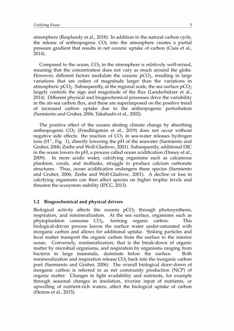
For the sea surface, the Surface Ocean CO2 Atlas (SOCAT, Bakker et al.,2016) compiles and quality controls measurements from global underwayships, as well as fixed moorings and drifting buoys (Fig. 2a). The large

Unifying Essay 5

majority of these measurements are collected from programs such asVoluntary Observing Ships and among other variables, this databasecontains pCO2 data that are used to compute the air-sea carbon flux. Mostof the SOCAT measurements are taken autonomously using an equilibratorwith a continuous sea-water flow (Bakker et al., 2016). Here, the pCO2 is notmeasured directly, but the mole fraction of CO2 (xCO2 in parts per million)is measured, from which the pCO2 (in µatm) can be inferred.

For the water column, the Global Ocean Data Analysis Project for Carbon(GLODAP, Olsen et al., 2019; Key et al., 2015) compiles and quality controlsglobal ship measurements of carbonate system parameters at depth (Fig.2b). The DIC is directly measured using bottled sea-water samples that areanalyzed in the laboratory. There are some research cruises as part ofGLODAP that did not measure the DIC directly; there, the DIC wascalculated based on pH and alkalinity measurements from bottled samples.As the system of measuring DIC is not autonomous, there are substantiallyfewer measurements of DIC available than of the surface carbonparameters, such as pCO2 (Fig. 2). However, locations with measurementshave often been sampled multiple times through the repeat hydrographysurveys that include the World Ocean Circulation Experiment (WOCE,http://woceatlas.ucsd.edu/) in the 1990s and CLIVAR(http://www.clivar.org/) since the 2000s (Talley et al., 2016).

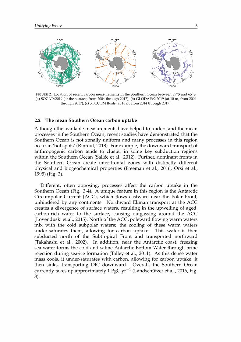
Since 2014, Argo floats equipped with biogeochemical sensors, as a newtype of in-situ observing platform, have substantially increased the numberof carbon measurements in the Southern Ocean. As part of the SouthernOcean Carbon and Climate Observations and Modeling project (SOCCOM,https://soccom.princeton.edu/, Fig. 2c), these robotic floats measuretemperature, conductivity (for salinity), pressure (for depth), pH, oxygen,nitrate, and bio-optics. The DIC can then be calculated using the CO2SYSanalysis tool (Heuven et al., 2011) with pH measurements from the floatsand total alkalinity estimated, for example, with temperature and salinitymeasurements and the LIAR algorithm (Carter et al., 2018). Approximately200 of these autonomous floats have been deployed in the Southern Oceanto complement shipboard measurements. In the four years from 2014through 2017, the SOCCOM floats have already considerably increased thespatio-temporal resolution of carbon measurements in the Southern Ocean(Fig. 2).

Unifying Essay 6

FIGURE 2: Location of recent carbon measurements in the Southern Ocean between 35◦S and 65◦S.(a) SOCATv2019 (at the surface, from 2004 through 2017); (b) GLODAPv2.2019 (at 10 m, from 2004

through 2017); (c) SOCCOM floats (at 10 m, from 2014 through 2017).

2.2 The mean Southern Ocean carbon uptake

Although the available measurements have helped to understand the meanprocesses in the Southern Ocean, recent studies have demonstrated that theSouthern Ocean is not zonally uniform and many processes in this regionoccur in ’hot spots’ (Rintoul, 2018). For example, the downward transport ofanthropogenic carbon tends to cluster in some key subduction regionswithin the Southern Ocean (Sallée et al., 2012). Further, dominant fronts inthe Southern Ocean create inter-frontal zones with distinctly differentphysical and biogeochemical properties (Freeman et al., 2016; Orsi et al.,1995) (Fig. 3).

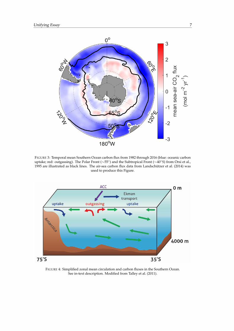
Different, often opposing, processes affect the carbon uptake in theSouthern Ocean (Fig. 3-4). A unique feature in this region is the AntarcticCircumpolar Current (ACC), which flows eastward near the Polar Front,unhindered by any continents. Northward Ekman transport at the ACCcreates a divergence of surface waters, resulting in the upwelling of aged,carbon-rich water to the surface, causing outgassing around the ACC(Lovenduski et al., 2015). North of the ACC, poleward flowing warm watersmix with the cold subpolar waters; the cooling of these warm watersunder-saturates them, allowing for carbon uptake. This water is thensubducted north of the Subtropical Front and transported northward(Takahashi et al., 2002). In addition, near the Antarctic coast, freezingsea-water forms the cold and saline Antarctic Bottom Water through brinerejection during sea-ice formation (Talley et al., 2011). As this dense watermass cools, it under-saturates with carbon, allowing for carbon uptake; itthen sinks, transporting DIC downward. Overall, the Southern Oceancurrently takes up approximately 1 PgC yr−1 (Landschützer et al., 2016, Fig.3).

Unifying Essay 7

FIGURE 3: Temporal mean Southern Ocean carbon flux from 1982 through 2016 (blue: oceanic carbonuptake; red: outgassing). The Polar Front (∼55◦) and the Subtropical Front (∼40◦S) from Orsi et al.,1995 are illustrated as black lines. The air-sea carbon flux data from Landschützer et al. (2014) was

used to produce this Figure.

FIGURE 4: Simplified zonal mean circulation and carbon fluxes in the Southern Ocean.See in-text description. Modified from Talley et al. (2011).

Unifying Essay 8

2.3 Southern Ocean carbon uptake variability

While the processes involving the mean Southern Ocean carbon sink aregenerally well understood, the variability of these processes is not. Recentstudies of the CO2 uptake in the Southern Ocean have suggested a largecarbon sink variability on interannual to decadal timescales, which is notcaptured by models (Frölicher et al., 2015) and the physical processes anddrivers contributing to this variability in the various sectors of the SouthernOcean are still debated (DeVries et al., 2017; Landschützer et al., 2015;Le Quéré et al., 2007).

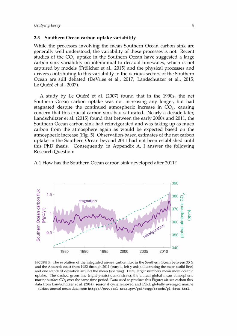
A study by Le Quéré et al. (2007) found that in the 1990s, the netSouthern Ocean carbon uptake was not increasing any longer, but hadstagnated despite the continued atmospheric increase in CO2, causingconcern that this crucial carbon sink had saturated. Nearly a decade later,Landschützer et al. (2015) found that between the early 2000s and 2011, theSouthern Ocean carbon sink had reinvigorated and was taking up as muchcarbon from the atmosphere again as would be expected based on theatmospheric increase (Fig. 5). Observation-based estimates of the net carbonuptake in the Southern Ocean beyond 2011 had not been established untilthis PhD thesis. Consequently, in Appendix A, I answer the followingResearch Question:

A.1 How has the Southern Ocean carbon sink developed after 2011?

FIGURE 5: The evolution of the integrated air-sea carbon flux in the Southern Ocean between 35°Sand the Antarctic coast from 1982 through 2011 (purple, left y-axis), illustrating the mean (solid line)and one standard deviation around the mean (shading). Here, larger numbers mean more oceanicuptake. The dashed green line (right y-axis) demonstrates the annual global mean atmosphericmarine surface CO2 over the same time period. Data used to produce this Figure: air-sea carbon fluxdata from Landschützer et al. (2014), seasonal cycle removed and ESRL globally averaged marine

surface annual mean data from https://www.esrl.noaa.gov/gmd/ccgg/trends/gl_data.html.

Unifying Essay 9

Several different processes have been proposed as potential drivers forthis large interannual to decadal variability. The Southern Annular Mode(SAM), defined as the zonal pressure difference between 40◦S and 65◦S, isthe dominant mode of climate variability in the southern high latitudes(Marshall, 2003). There has been a positive trend in the SAM in recentdecades, causing a strengthening and poleward shift of the westerly winds(Hall and Visbeck, 2002). These strengthened winds lead to enhancedoutgassing which Le Quéré et al. (2007) argued led to the stagnation of thenet Southern Ocean carbon uptake in the 1990s. However, the positive trendin the SAM has continued beyond the stagnation period, but the SouthernOcean carbon sink did not continue to stagnate. Another proposed driver ofthe Southern Ocean carbon sink variability is based on recently observedchanges in the upper Meridional Overturning Circulation (MOC, DeVrieset al., 2017). That study argued that a slow-down in the MOC had led to anoverall increase in oceanic carbon uptake in the 1990s through lessoutgassing of natural carbon. That weakening was followed by a strongerMOC in the 2000s, which decreased the net carbon uptake throughenhanced outgassing. In addition, the reinvigoration in the 2000s has alsobeen also linked to a zonally asymmetric atmospheric circulation thatenhanced the CO2 uptake in that period (Landschützer et al., 2015). Gregoret al. (2018) argued that biological activity drives the Southern Ocean carbonsink variability in austral summer, and wind stress in austral winter.Bronselaer et al. (2020) found that besides the positive trend in the SAM,increased melting of the Antarctic ice sheet in recent years has led toincreases in oceanic carbon content in the water column. The relativeimportance of the potential drivers of the carbon uptake variability in theSouthern Ocean is, however, still debated. Thus, in Appendix A, I addressthe following Research Question:

A.2 What are the drivers behind the recent interannual variability of theSouthern Ocean carbon sink?

2.4 Variability in interior Southern Ocean DIC

Previous studies of changes in the oceanic carbon at depth have focused onthe uptake of anthropogenic carbon and the decadal changes thereof(Clement and Gruber, 2018; Gruber et al., 2019b; Khatiwala et al., 2009;Sabine et al., 2004). Most recently, Gruber et al. (2019b) found that althoughthe Southern Ocean took up approximately 1 PgC yr−1, between 1994 and2007, only approximately 0.6 PgC yr−1 was stored in this region as DIC,while the rest was transported northward, leaving the Southern Ocean(DeVries, 2014; Gruber et al., 2019a; Mikaloff Fletcher et al., 2006).

Due to different processes being dominant in sub-regions of the SouthernOcean, regional studies taking mapped fields into consideration arenecessary to fully reflect the different processes in the Southern Ocean. Thisstudy is the first observation-based study that includes the Southern Oceanat regional scale to investigate the temporal changes in DIC on time-scales

Unifying Essay 10

shorter than decadal, or changes in contemporary (natural + anthropogenic)DIC on any time-scale. Subsequently, in Appendices B and C, I answer thefollowing Research Questions:

B.1 Can we map time-varying fields of DIC using sparse ship data to createa monthly climatology?

C.1 Can we map time-varying fields of DIC in the Southern Ocean atinterannual monthly resolution?

Knowing about the changes in Southern Ocean DIC allows for ananalysis of these changes, thereby contributing to our collectiveunderstanding of the global carbon cycle and the processes involved. Thus,in Appendix C, I delve into the data estimate of monthly DIC from 2004through 2017 to answer the following Research Questions:

C.2 What is the extent of the variability of DIC in the water column?

C.3 What are the drivers behind the variability of DIC at the surface andbelow?

3 Machine Learning

As traditional interpolation methods, such as optimal interpolations, hadbeen unable to resolve time-varying global mapped fields of surface carbonmeasurements, various interpolation and mapping methods have recentlyemerged, ranging from statistical auto-correlation techniques to machinelearning approaches (Jones et al., 2015; Landschützer et al., 2013; Rödenbecket al., 2015). In the field of machine learning, computational algorithms arestatistically trained to classify, predict, cluster, or discover patterns in adataset (Reichstein et al., 2019). Neural networks, a sub-branch of machinelearning, can be used to reconstruct and map data that have spatio-temporalgaps (Gardner and Dorling, 1998).

3.1 Terminology

As the terms gridded, interpolated, and mapped data are often usedinterchangeably, I first briefly define them here, following the work byLauvset et al. (2016).

Observations are often projected onto a regular grid, using binning andaveraging, but without interpolation or calculations to fill empty grid cells.One such example is the gridded dataset of SOCAT data (Bakker et al., 2016)by Sabine et al. (2013). In a classical interpolation, the original observationsdo not change, and values are only added between the data gaps, hencethere are no residuals in interpolations. One such example is the verticalinterpolation commonly performed to bring ship-based observations onto

Unifying Essay 11

standard depth levels and Cubic Hermite functions are commonly used forthese interpolations. In a mapped data product, observational gaps are filledusing some form of interpolation or other mapping approaches to produce agap-filled map. In some mapping approaches, such as the one describedbelow, each grid cell, including those containing the original griddedobservations, is computed. In such an approach there are residuals betweenthe observations and the mapped values, which are set to be minimal.

3.2 SOM-FFN

Landschützer et al. (2013) developed a two-step neural network mappingapproach to overcome the low spatio-temporal density of surface carbonmeasurements. In their SOM-FFN approach, the authors first useself-organizing maps (SOMs) to cluster the oceans into regions of similarbiogeochemical properties, and in a second step, they run a feed-forwardnetwork (FFN) in each of the clusters to compute and apply the statisticalrelationship between pCO2 and specific predictor data. The predictor dataare more numerous and spread more evenly around the world than thetarget data (pCO2), thereby helping to overcome the low spatio-temporaldensity of surface carbon measurements.

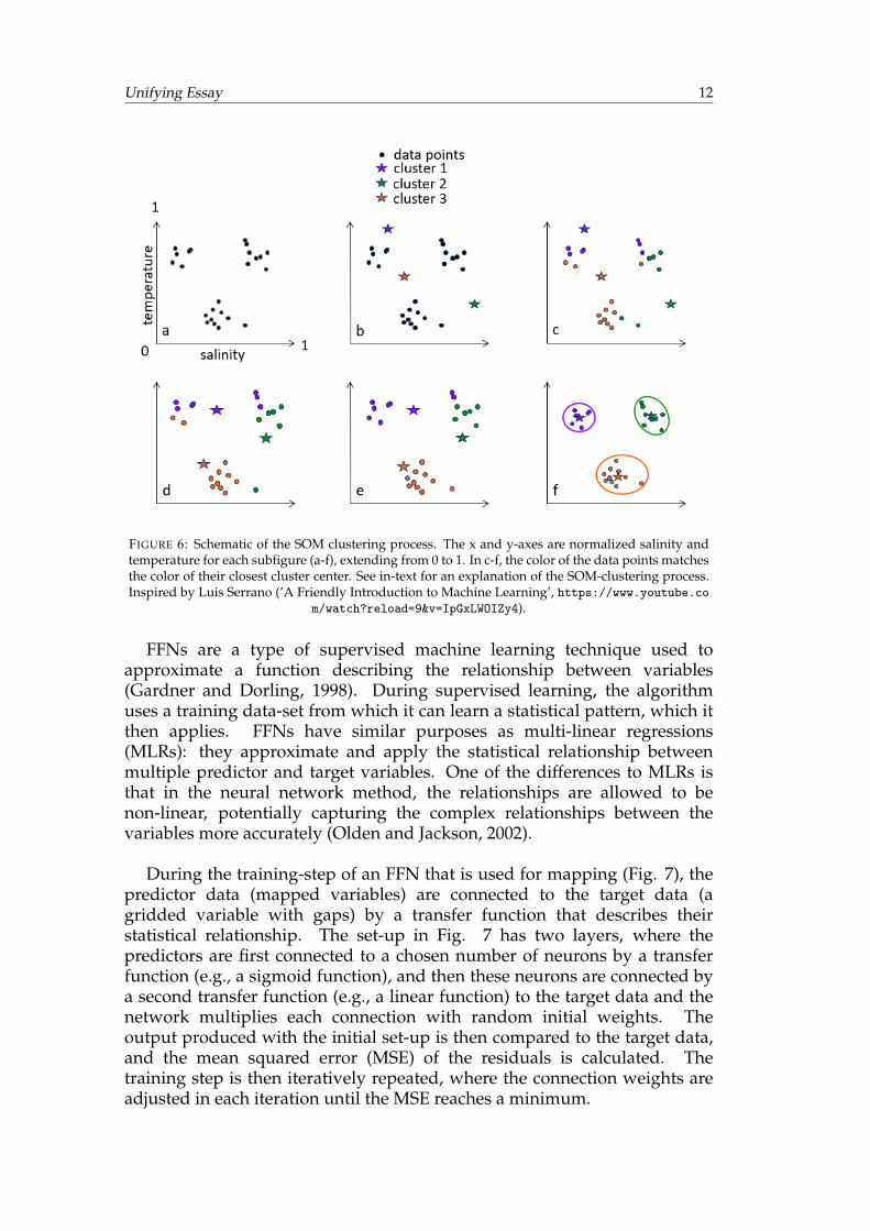
SOMs are a type of unsupervised machine learning technique to clusterdata (Kohonen, 1989; Kohonen, 2001). During unsupervised learning, thealgorithm looks for patterns in a data set, that were not labeled as suchbefore. The SOM-clustering process is as follows (Fig. 6): the variables thatare to be clustered—in the schematic temperature and salinity—are usuallyfirst normalized (Fig. 6a) and the user prescribes the number of desiredclusters (in the schematic: three). The algorithm begins by placing proposedcluster centers randomly in the grid space around the input variables andcalculates the Euclidean distance between the input variables and theirclosest cluster center (Fig. 6b). Next, the centers are iteratively movedaround to minimize the sum of the distances of all the input variables totheir closest cluster center (Fig. 6c-f). The user prescribes a maximumnumber of iterations, but the algorithm stops before that number is reachedif the distances cannot be minimized further (Fig. 6f).

Unifying Essay 12

FIGURE 6: Schematic of the SOM clustering process. The x and y-axes are normalized salinity andtemperature for each subfigure (a-f), extending from 0 to 1. In c-f, the color of the data points matchesthe color of their closest cluster center. See in-text for an explanation of the SOM-clustering process.Inspired by Luis Serrano (’A Friendly Introduction to Machine Learning’, https://www.youtube.co

m/watch?reload=9&v=IpGxLWOIZy4).

FFNs are a type of supervised machine learning technique used toapproximate a function describing the relationship between variables(Gardner and Dorling, 1998). During supervised learning, the algorithmuses a training data-set from which it can learn a statistical pattern, which itthen applies. FFNs have similar purposes as multi-linear regressions(MLRs): they approximate and apply the statistical relationship betweenmultiple predictor and target variables. One of the differences to MLRs isthat in the neural network method, the relationships are allowed to benon-linear, potentially capturing the complex relationships between thevariables more accurately (Olden and Jackson, 2002).

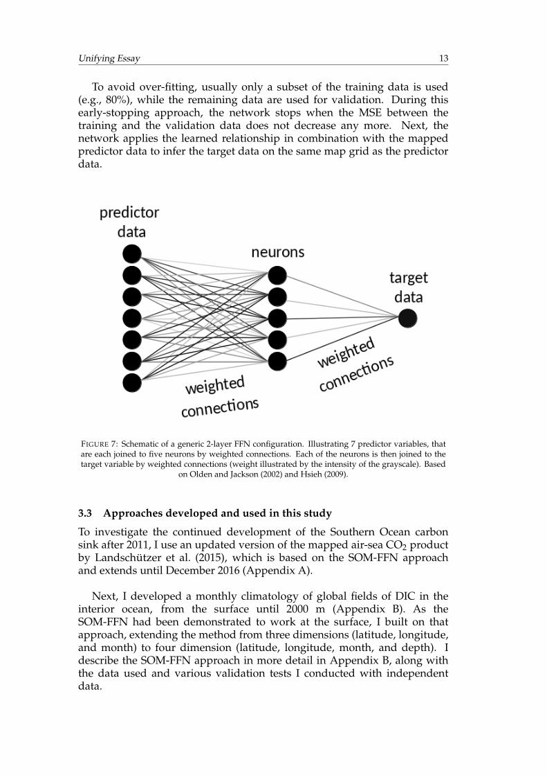
During the training-step of an FFN that is used for mapping (Fig. 7), thepredictor data (mapped variables) are connected to the target data (agridded variable with gaps) by a transfer function that describes theirstatistical relationship. The set-up in Fig. 7 has two layers, where thepredictors are first connected to a chosen number of neurons by a transferfunction (e.g., a sigmoid function), and then these neurons are connected bya second transfer function (e.g., a linear function) to the target data and thenetwork multiplies each connection with random initial weights. Theoutput produced with the initial set-up is then compared to the target data,and the mean squared error (MSE) of the residuals is calculated. Thetraining step is then iteratively repeated, where the connection weights areadjusted in each iteration until the MSE reaches a minimum.

Unifying Essay 13

To avoid over-fitting, usually only a subset of the training data is used(e.g., 80%), while the remaining data are used for validation. During thisearly-stopping approach, the network stops when the MSE between thetraining and the validation data does not decrease any more. Next, thenetwork applies the learned relationship in combination with the mappedpredictor data to infer the target data on the same map grid as the predictordata.

FIGURE 7: Schematic of a generic 2-layer FFN configuration. Illustrating 7 predictor variables, thatare each joined to five neurons by weighted connections. Each of the neurons is then joined to thetarget variable by weighted connections (weight illustrated by the intensity of the grayscale). Based

on Olden and Jackson (2002) and Hsieh (2009).

3.3 Approaches developed and used in this study

To investigate the continued development of the Southern Ocean carbonsink after 2011, I use an updated version of the mapped air-sea CO2 productby Landschützer et al. (2015), which is based on the SOM-FFN approachand extends until December 2016 (Appendix A).

Next, I developed a monthly climatology of global fields of DIC in theinterior ocean, from the surface until 2000 m (Appendix B). As theSOM-FFN had been demonstrated to work at the surface, I built on thatapproach, extending the method from three dimensions (latitude, longitude,and month) to four dimension (latitude, longitude, month, and depth). Idescribe the SOM-FFN approach in more detail in Appendix B, along withthe data used and various validation tests I conducted with independentdata.

Unifying Essay 14

To investigate the interannual variability of DIC in the interior SouthernOcean, I further built on the method from Appendix B, increasing thetemporal resolution to create a second data set, which consists of globalmapped fields of interior DIC with monthly temporal resolution from 2004through 2017, from the surface until 500 m (Appendix C).

In my SOM-FFN set-up, the target data of the FFN are the sparse shipmeasurements of DIC, while the predictor data are better-constrainedvariables that are related to DIC (e.g., temperature, salinity, dissolvedoxygen, and nutrients). These variables exist at a higher spatio-temporaldensity than DIC measurements, and so, mapped time-varying dataproducts of these variables have been produced using traditionalinterpolation techniques, such as optimal interpolations.

Mapping the interior DIC poses additional challenges compared tomapping the surface pCO2. First, the DIC measurements at depth are evensparser than surface carbon measurements (Fig. 2). Second, while manypredictors can be used at the surface, for example, from satelliteobservations, very few variables are available as predictors at depth.Despite these challenges, the method passes relevant validation tests andcan adequately map the time-varying DIC fields, as demonstrated inAppendices B and C.

4 Summary of Key Results

4.1 Interannual variability of Southern Ocean carbon fluxes

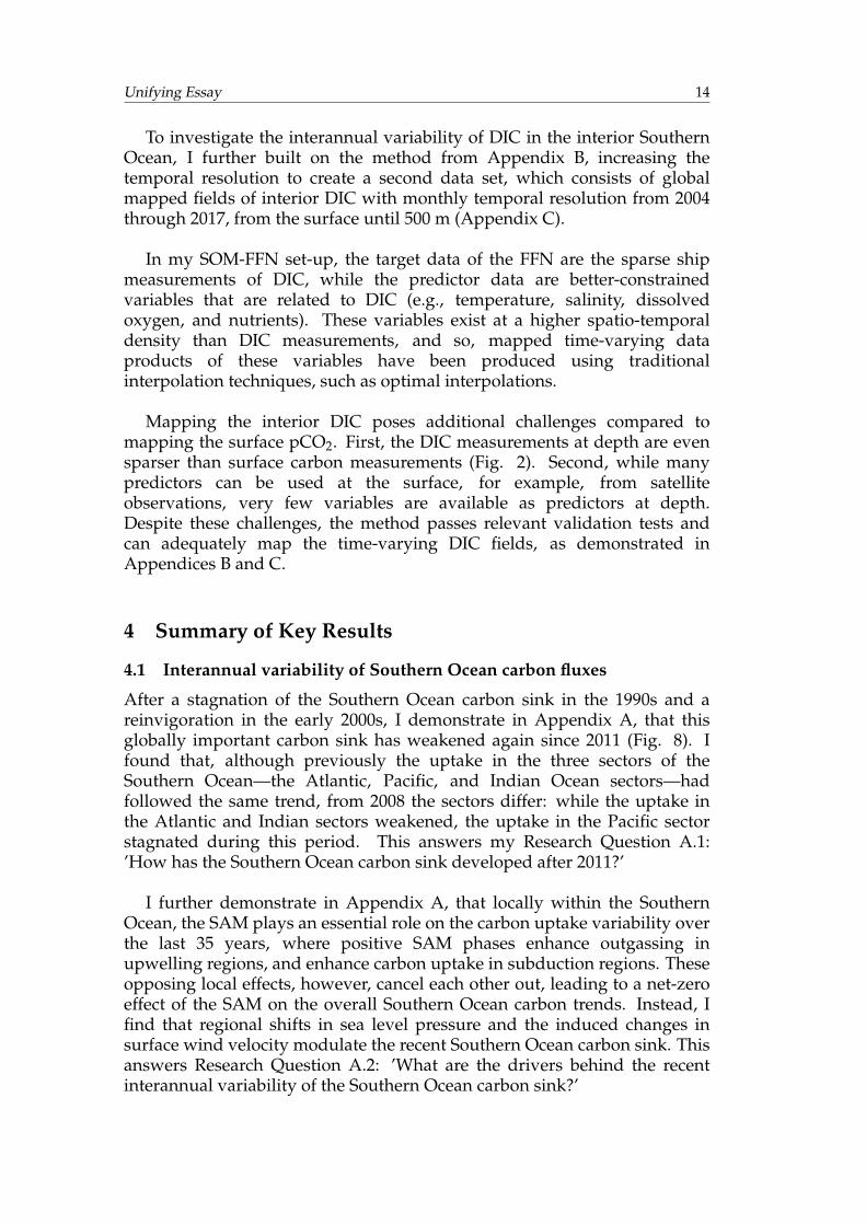
After a stagnation of the Southern Ocean carbon sink in the 1990s and areinvigoration in the early 2000s, I demonstrate in Appendix A, that thisglobally important carbon sink has weakened again since 2011 (Fig. 8). Ifound that, although previously the uptake in the three sectors of theSouthern Ocean—the Atlantic, Pacific, and Indian Ocean sectors—hadfollowed the same trend, from 2008 the sectors differ: while the uptake inthe Atlantic and Indian sectors weakened, the uptake in the Pacific sectorstagnated during this period. This answers my Research Question A.1:’How has the Southern Ocean carbon sink developed after 2011?’

I further demonstrate in Appendix A, that locally within the SouthernOcean, the SAM plays an essential role on the carbon uptake variability overthe last 35 years, where positive SAM phases enhance outgassing inupwelling regions, and enhance carbon uptake in subduction regions. Theseopposing local effects, however, cancel each other out, leading to a net-zeroeffect of the SAM on the overall Southern Ocean carbon trends. Instead, Ifind that regional shifts in sea level pressure and the induced changes insurface wind velocity modulate the recent Southern Ocean carbon sink. Thisanswers Research Question A.2: ’What are the drivers behind the recentinterannual variability of the Southern Ocean carbon sink?’

Unifying Essay 15

FIGURE 8: Extension of the evolution of the Southern Ocean carbon flux per unit area, between 35°Sand the Antarctic coast from 1982 through 2016 in the Atlantic (green), Pacific (purple), and Indian

(orange) sectors.

4.2 Monthly climatology of global interior DIC

In Appendix B, I demonstrate that it is possible to map time-varying fieldsof interior DIC using sparse ship data. I created a monthly climatology ofDIC from the sea-surface to 2000 m, using a 2-step neural-network-basedmapping technique and DIC measurements from the GLODAPv2.2019 dataproduct. Various tests with an ocean biogeochemistry model, and withindependent observations that were not used to train the networkdemonstrate that the method can capture the seasonal cycle of DIC at globalscale with an average root mean squared error (RMSE) of approximately 20µmol kg−1. This answers my Research Question B.1: ’Can we maptime-varying fields of DIC using sparse ship data to create a monthlyclimatology?’

In addition to answering the main research questions in this dissertation,I also describe the global seasonal carbon dynamics using my new dataproduct in Appendix B. As the largest signal in the changes in DIC is theseasonal cycle, it considerably affects the amount of carbon taken up by theocean. A study by Mongwe et al. (2018) demonstrated that the CoupledModel Intercomparison Project phase 5 (CMIP5) models disagree on thephase and amplitude of Southern Ocean inorganic carbon, while Nevisonet al. (2016) highlighted that the seasonal carbon dynamics in the CMIP5models significantly affect their climate projections. Thus, understandingthe seasonal carbon dynamics and the underlying processes forms animportant part of climate research.

Unifying Essay 16

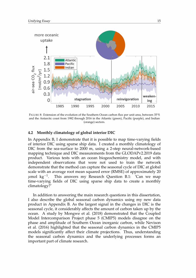
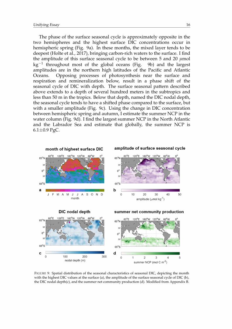
The phase of the surface seasonal cycle is approximately opposite in thetwo hemispheres and the highest surface DIC concentrations occur inhemispheric spring (Fig. 9a). In these months, the mixed layer tends to bedeepest (Holte et al., 2017), bringing carbon-rich waters to the surface. I findthe amplitude of this surface seasonal cycle to be between 5 and 20 µmolkg−1 throughout most of the global oceans (Fig. 9b) and the largestamplitudes are in the northern high latitudes of the Pacific and AtlanticOceans. Opposing processes of photosynthesis near the surface andrespiration and remineralization below, result in a phase shift of theseasonal cycle of DIC with depth. The surface seasonal pattern describedabove extends to a depth of several hundred meters in the subtropics andless than 50 m in the tropics. Below that depth, named the DIC nodal depth,the seasonal cycle tends to have a shifted phase compared to the surface, butwith a smaller amplitude (Fig. 9c). Using the change in DIC concentrationbetween hemispheric spring and autumn, I estimate the summer NCP in thewater column (Fig. 9d). I find the largest summer NCP in the North Atlanticand the Labrador Sea and estimate that globally, the summer NCP is6.1±0.9 PgC.

FIGURE 9: Spatial distribution of the seasonal characteristics of seasonal DIC, depicting the monthwith the highest DIC values at the surface (a), the amplitude of the surface seasonal cycle of DIC (b),the DIC nodal depth(c), and the summer net community production (d). Modified from Appendix B.

Unifying Essay 17

4.3 Interannual variability of interior Southern Ocean DIC

In Appendix C, I build on the method from Appendix B, extending thetemporal resolution to monthly mapped fields of DIC at global scale from2004 through 2017. Focusing on the Southern Ocean, I test this new dataestimate with independent data and find that the method adequately mapsthe Southern Ocean DIC, capturing its mean, trend, and interannualvariability, illustrated by the RMSE of 24 µmol kg−1 between my DICestimate and the DIC calculated from SOCCOM floats. In addition, testswith synthetic data from the ocean biogeochemistry model HAMOCC(Ilyina et al., 2013; Mauritsen et al., 2019) demonstrate that our estimate canreconstruct the model field with an RMSE of 8 µmol kg−1. This answersResearch Question C.1: ’Can we map time-varying fields of DIC in theSouthern Ocean at interannual monthly resolution?’

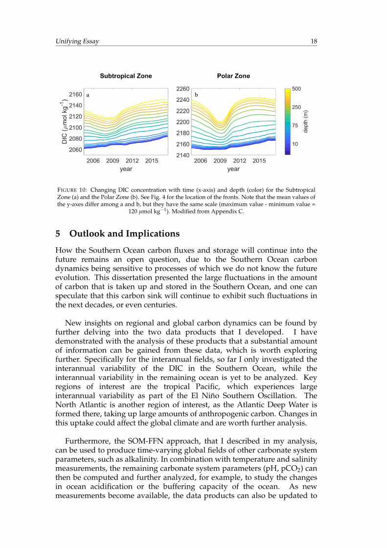
Analyzing this new data estimate of monthly mapped DIC fields, I findthat the surface DIC has a very weak interannual variability compared tothe air-sea CO2 flux, and the strongest signal here is theanthropogenically-driven positive trend. Below the surface, my analysisreveals a large temporary sub-surface reduction in DIC from 2004 until theyear 2009, which is followed by a recovery until 2012 (Fig. 10). Thisreduction is the strongest south of the Polar Front, i.e., near the Antarcticcoast, and extends to 500 m. This answers Research Question C.2: ’What isthe extent of the variability of DIC in the water column?’

I present multiple lines of evidence that link this temporary reduction insub-surface DIC to recent changes in the MOC. A weakening overturningcirculation in the 2000s led to less upwelling of Southern Ocean DIC,creating the sub-surface reduction, allowing for additional carbon uptake atthe surface. While we do not know the evolution of the MOC after 2009, it islikely that enhanced upwelling aided the recovery of the sub-surfacereduction in DIC, and weakened the carbon uptake at the surface. Thisanswers Research Question C.3: ’What are the drivers behind the variabilityof DIC at the surface and below?’

4.4 Drivers of variability at the surface and below

In Appendix A, I find that the SAM does not have an overall effect on therecent variability in the air-sea carbon uptake, integrated over the wholeSouthern Ocean. Conversely, in Appendix C, I attribute the variability insub-surface DIC to changes in the MOC, which is tied to the SAM. Thesefindings demonstrate that in positive SAM phases, the regional effects ofenhanced outgassing in regions of upwelling is counter-balanced byenhanced uptake elsewhere at the surface, which creates the overall net-zeroeffect of the SAM on the Southern Ocean carbon flux. However, below thesurface, the reduced upward transport is visible in the DIC pool, asdemonstrated in Appendix C.

Unifying Essay 18

FIGURE 10: Changing DIC concentration with time (x-axis) and depth (color) for the SubtropicalZone (a) and the Polar Zone (b). See Fig. 4 for the location of the fronts. Note that the mean values ofthe y-axes differ among a and b, but they have the same scale (maximum value - minimum value =

120 µmol kg−1). Modified from Appendix C.

5 Outlook and Implications

How the Southern Ocean carbon fluxes and storage will continue into thefuture remains an open question, due to the Southern Ocean carbondynamics being sensitive to processes of which we do not know the futureevolution. This dissertation presented the large fluctuations in the amountof carbon that is taken up and stored in the Southern Ocean, and one canspeculate that this carbon sink will continue to exhibit such fluctuations inthe next decades, or even centuries.

New insights on regional and global carbon dynamics can be found byfurther delving into the two data products that I developed. I havedemonstrated with the analysis of these products that a substantial amountof information can be gained from these data, which is worth exploringfurther. Specifically for the interannual fields, so far I only investigated theinterannual variability of the DIC in the Southern Ocean, while theinterannual variability in the remaining ocean is yet to be analyzed. Keyregions of interest are the tropical Pacific, which experiences largeinterannual variability as part of the El Niño Southern Oscillation. TheNorth Atlantic is another region of interest, as the Atlantic Deep Water isformed there, taking up large amounts of anthropogenic carbon. Changes inthis uptake could affect the global climate and are worth further analysis.

Furthermore, the SOM-FFN approach, that I described in my analysis,can be used to produce time-varying global fields of other carbonate systemparameters, such as alkalinity. In combination with temperature and salinitymeasurements, the remaining carbonate system parameters (pH, pCO2) canthen be computed and further analyzed, for example, to study the changesin ocean acidification or the buffering capacity of the ocean. As newmeasurements become available, the data products can also be updated to

Unifying Essay 19

extend further in time, allowing for continuous monitoring of the carbonuptake and storage, as well as its drivers.

It is worth noting that the potential drivers on the Southern Ocean carbonvariability are difficult to disentangle based on observations. As correlationdoes not imply causation, it is challenging to determine which drivers arenecessary and which are sufficient. A necessary cause would be an event,without which the consequence cannot occur, while a sufficient cause wouldbe an event that is always followed by the consequence (Pearl, 2016). EarthSystem Models are potentially capable tools to disentangle these factorswith sensitivity analyses (Pearl, 2016). However, as models currently tend tounderestimate the observed variability (Frölicher et al., 2015), first they haveto be able to capture this variability before being able to disentangle itsdrivers.

Another opportunity for further research is the analysis of the statisticaldrivers of the seasonal cycle of DIC in observations and models. DifferentCMIP5 models substantially disagree on the phase and amplitude of theseasonal cycle of inorganic carbon in the Southern Ocean (Mongwe et al.,2018). Using the method from Appendix B (Fig. B.7), the seasonal responsefunction from the Neural Network in the Southern Ocean could be derivedin models to determine the statistical drivers of DIC in these models. Thismethod could, for example, be applied with different Coupled ModelIntercomparison Project (CMIP) models to provide us insights into whichmodels best represent the seasonal cycle of DIC in the Southern Ocean anddemonstrate statistically why they do so (e.g., the biology or circulationcould be too strong or too weak as a driver). This information could then beused to understand the carbon cycle better and improve climate projections.

Due to the global importance of the Southern Ocean carbon sink(Friedlingstein et al., 2019; Frölicher et al., 2015), the findings from thisdissertation are crucial for the sustained monitoring and understanding ofnot only the Southern Ocean carbon sink, but also of the global carbon cycle,essential for governmental and economic decisions on carbon emissionreduction pathways.

20

Appendices

AppendixA: Keppler, L. and P. Landschützer (2019). "Regional WindVariability Modulates the Southern Ocean Carbon Sink". In: ScientificReports 9, 7384. DOI: 10.1038/s41598-019-43826-y.

Appendix B: Keppler, L., P. Landschützer, N. Gruber, S.K. Lauvset, I.Stemmler (in review). "Seasonal Carbon Dynamics in the Global Oceanbased on a Neural-Network Mapping of Observations". In review at GlobalBiogeochemical Cycles.

Appendix C: Keppler, L. and P. Landschützer (in prep.). "TemporaryReduction in Southern Ocean sub-surface Dissolved Inorganic Carbon". Tobe submitted to Geophysical Research Letters.

21

A Regional Wind Variability Modulates the Southern OceanCarbon Sink

Keppler, Lydia1,2 & Peter Landschützer1

1 Max-Planck-Institute for Meteorology (MPI-M), Hamburg, Germany.2 International Max Planck Research School on Earth System Modelling(IMPRS-ESM), Hamburg, Germany.

Paper status: Published online on 14 May 2019 in Scientific Reports (2019)9:7384 https://www.nature.com/articles/s41598-019-43826-y.

Data availability: The datasets generated during the current study areavailable from NOAA OCADS (https://www.nodc.noaa.gov/ocads/oceans/SPCO$_2$_1982_present_ETH_SOM_FFN.html). All remaining dataanalysed during this study are included in this published article (and itsSupplementary Information files).

Supplementary Information accompanies this paper (see online version).

Contributions: L.K. and P.L. designed the research; L.K. performed the research andanalysed the data; P.L. developed the CO2 data product. L.K. wrote the draftmanuscript;P.L. contributed to the discussion of the results and the manuscript atall stages.

Appendix A 22

Abstract

The Southern Ocean south of 35◦S accounts for approximately half of theannual anthropogenic carbon uptake by the ocean, thereby substantiallymitigating the effects of anthropogenic carbon dioxide (CO2) emissions. Theintensity of this important carbon sink varies considerably on interannual todecadal timescales. However, the drivers of this variability are still debated,challenging our ability to accurately predict the future role of the SouthernOcean in absorbing atmospheric carbon. Analysing mapped sea-air CO2fluxes, estimated from upscaled surface ocean CO2 measurements, we findthat the overall Southern Ocean carbon sink has weakened since ∼2011,reversing the trend of the reinvigoration period of the 2000s. Although wefind significant regional positive and negative responses of the SouthernOcean carbon uptake to changes in the Southern Annular Mode (SAM) overthe past 35 years, the net effect of the SAM on the Southern Ocean carbonsink variability is approximately zero, due to the opposing effects ofenhanced outgassing in upwelling regions and enhanced carbon uptakeelsewhere. Instead, regional shifts in sea level pressure, linked to zonalwavenumber 3 (ZW3) and related changes in surface winds substantiallycontribute to the interannual to decadal variability of the Southern Oceancarbon sink.

1 Introduction

The global oceans absorb ∼25% of the annually emitted carbon dioxide(CO2) from human activities (Le Quéré et al., 2018). A disproportionallylarge part of this uptake is linked to the Southern Ocean south of 35◦S,which accounts for ∼50% of the annual oceanic CO2 uptake (Landschützeret al., 2016) and where ∼40% of all emitted anthropogenic CO2 since thebeginning of industrialisation is stored (Frölicher et al., 2015; Khatiwalaet al., 2009; Sabine et al., 2004). Therefore, the Southern Ocean plays asubstantial role in mitigating the effects of human carbon emissions andunderstanding this carbon sink and its related processes is crucial for futureclimate projections.

A sobering study by Le Quéré et al. (2007) showed that despite thecontinued increase in atmospheric CO2, the Southern Ocean carbon sinksaturated in the 1990s, diverging from the expected uptake based onthermodynamic considerations. The authors explained this saturation witha positive trend in the Southern Annular Mode (SAM), i.e., the dominantmode of variability in the Southern Ocean, describing the zonal pressuredifference between 40◦S and 65◦S (Marshall, 2003). This positive trend led toan intensification and poleward shift of the westerly winds, the drivingforce behind the Southern Ocean upwelling of carbon-rich deep water(Marshall, 2003; Thompson and Solomon, 2002; Thompson et al., 2000). Thelink between the saturation of the Southern Ocean carbon sink in the 1990sand the positive SAM phase was later confirmed by other model andatmospheric inverse studies (Hauck et al., 2013; Lenton and Matear, 2007;

Appendix A 23

Lovenduski et al., 2008, 2007; Zickfeld et al., 2007).

Further studies have demonstrated that the response of the mixed-layerdepth and temperature to the SAM is not as “annular” (ring-shaped) aspreviously thought, and is in fact zonally asymmetric, possibly affecting theSouthern Ocean carbon uptake (Fogt et al., 2012; Sallée et al., 2010; see alsoSupplementary Information A_SI.1). Due to the scarcity of observationaldata, many previous studies focused on zonal averages of the wholeSouthern Ocean. Although this view has helped to understand the meandynamics in the last two decades, it is becoming more and more evidentthat the Southern Ocean is not zonally uniform and that many key processesoccur in different regions that are averaged out in zonal averages (Rintoul,2018; Sallée et al., 2012).

Recent technical advancements and efforts by the scientific communityhave led to basin-wide observation-based estimates of the sea-air CO2 flux,sea surface temperature (SST), and sea surface salinity (SSS). To overcomethe paucity of CO2 measurements, novel approaches based on statisticalrelationships and machine-learning algorithms have advanced our ability toextrapolate and basin-wide map the information collected from singlesampling routes (Landschützer et al., 2014).

Using the mapped partial pressure of CO2 (pCO2) data until December2011, a study established that the saturation trend of the 1990s stopped andreversed between the early 2000s and 2011 and that the Southern Ocean hadreturned to its expected uptake strength (Landschützer et al., 2015). Despitethe shipboard-based pCO2 estimates being heavily extrapolated,longer-term signals, such as the decadal fluctuations that mark thesaturation and reinvigoration periods were identified as robust featuresamong different approaches (Ritter et al., 2017; Rödenbeck et al., 2015), andthe reinvigoration of the Southern Ocean carbon sink was later confirmedby several other studies (DeVries et al., 2017; Gregor et al., 2018; Ritter et al.,2017).

Despite increasing evidence for the strengthening of the Southern Oceancarbon sink in the 2000s, the processes behind this strengthening are stilldebated, and the future evolution of this important sink region is highlyuncertain. One proposed mechanism is a zonally asymmetric atmosphericcirculation, which led to an oceanic dipole of warming and cooling that inturn increased the CO2 uptake during the Southern Ocean reinvigorationperiod (2002 through 2011; Landschützer et al., 2015). Another explanationis based on changes in the upper meridional overturning circulation (MOC),which may be linked to trends in the SAM (DeVries et al., 2017). Anotherstudy argues that the interannual drivers of the Southern Ocean carbon sinkare seasonally decoupled, with wind stress as the main driver in australwinter and biology in austral summer (Gregor et al., 2018).

Here, we build on previous assessments using neural-network derivedmapped pCO2 estimates based on shipboard measurements to demonstrate

Appendix A 24

the temporal evolution of the Southern Ocean carbon sink and its regionaldrivers. Finally, we focus on the period after the end of the reinvigoration in2011 and put our findings from this most recent period in context withprevious findings since the 1980s.

2 Results and Discussion

2.1 The Southern Ocean carbon sink variability

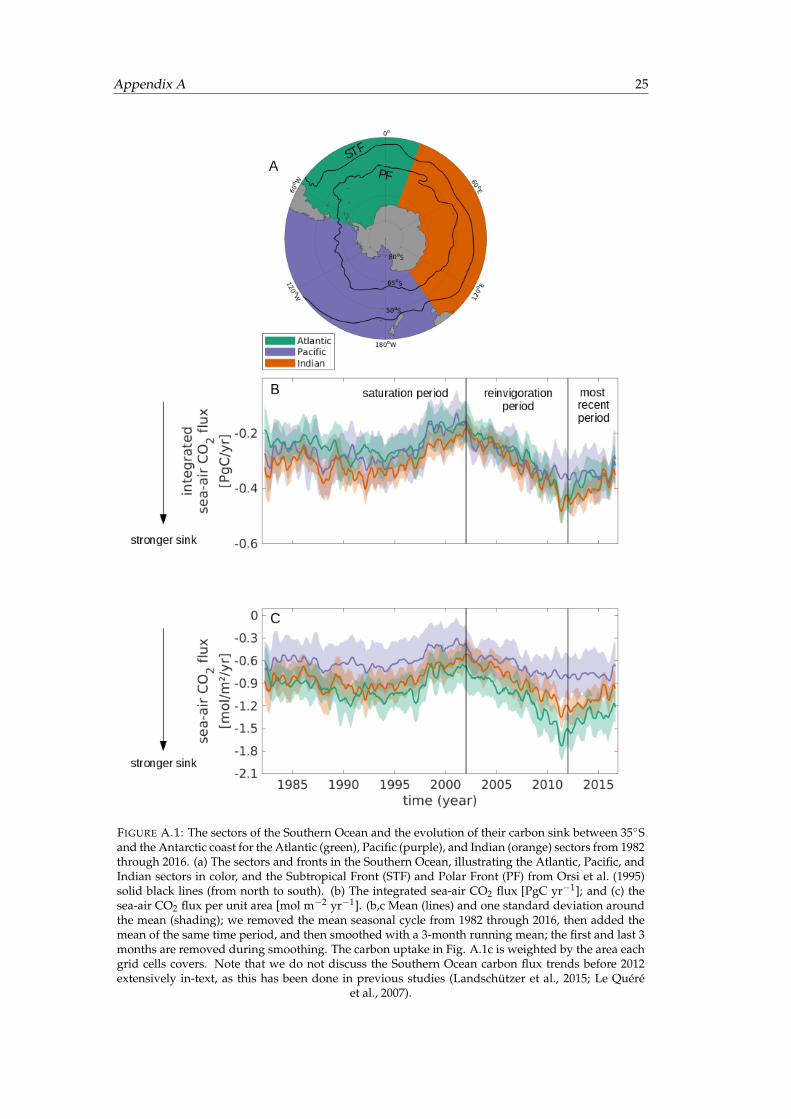
Using an updated observation-based mapped estimate of the sea-air CO2flux (extended from Landschützer et al. (2016)), we find that the substantialdecadal variability of the Southern Ocean carbon sink persists and is presentin all three sectors: the reinvigoration period of increased CO2 uptake lasteduntil ∼2011, and is followed by a reversal of this trend with decreasingcarbon uptake until the end of our study period in December 2016 (Fig.A.1b,c), consistent with a previous finding (Gregor et al., 2018).

The integrated CO2 uptake (Fig. A.1b) does not differ considerablybetween the three sectors despite the large differences in area (Atlanticsector: ∼2.2·107 km2, Pacific sector: ∼3.7·107 km2, and Indian sector:∼3.0·107 km2, Fig. A.1a). Specifically, the integrated sea-air CO2 flux from2012 through 2016 is approximately equal in each of the three sectors with amean uptake of 0.3 to 0.4 PgC yr−1 resulting in a total Southern Oceancarbon uptake of ∼1.1±0.2 PgC yr−1, or approx. 50% of the contemporaryannual mean oceanic carbon uptake. The comparable uptake strengthbetween sectors is in agreement with previous results, who found a fairlyhomogeneous carbon uptake between the three sectors from different modeland inversion estimates (Lenton et al., 2013).

Despite the sectoral similarities in the integrated CO2 uptake, strongsectoral differences exist in the magnitude of the sea-air CO2 flux per unitarea (Fig. A.1c). In particular, the Atlantic sector, i.e., the sector with thesmallest spatial extent, reveals the largest variability range from ∼-0.7 molm−2 yr−1 in the early 2000s to ∼-1.7 mol m−2 yr−1 in 2011. Throughoutmost of the time period, the Atlantic sector is the most intense carbon sinkper unit area within the Southern Ocean and from 2012 onward, the CO2uptake per unit area in the Atlantic sector (∼1.4 mol m−2 yr−1) is nearlytwice the amount taken up by the Pacific sector (∼0.8 mol m−2 yr−1) andstill considerably more than in the Indian sector (∼1.1 mol m−2 yr−1). Thisstrong mean uptake has been recently challenged using calculated pCO2from biogeochemical Argo floats (Gray et al., 2018; Williams et al., 2017).While the differences are not yet fully resolved, a combination of float andship data as a next step is required to fully constrain both the seasonal cycleand the mean uptake in the Southern Ocean. We therefore focus on theinterannual variability and regional differences rather than the integratedcarbon uptake in this study.

Appendix A 25

FIGURE A.1: The sectors of the Southern Ocean and the evolution of their carbon sink between 35◦Sand the Antarctic coast for the Atlantic (green), Pacific (purple), and Indian (orange) sectors from 1982through 2016. (a) The sectors and fronts in the Southern Ocean, illustrating the Atlantic, Pacific, andIndian sectors in color, and the Subtropical Front (STF) and Polar Front (PF) from Orsi et al. (1995)solid black lines (from north to south). (b) The integrated sea-air CO2 flux [PgC yr−1]; and (c) thesea-air CO2 flux per unit area [mol m−2 yr−1]. (b,c Mean (lines) and one standard deviation aroundthe mean (shading); we removed the mean seasonal cycle from 1982 through 2016, then added themean of the same time period, and then smoothed with a 3-month running mean; the first and last 3months are removed during smoothing. The carbon uptake in Fig. A.1c is weighted by the area eachgrid cells covers. Note that we do not discuss the Southern Ocean carbon flux trends before 2012extensively in-text, as this has been done in previous studies (Landschützer et al., 2015; Le Quéré

et al., 2007).

Appendix A 26

Another striking observation is that since the late 2000s, strongerdifferences between the sectors emerge. In the saturation period of the 1990sand the following reinvigoration period in the early 2000s, differencesbetween the sectors stay within one standard deviation around the mean,and they agree on the direction of the trend. However, since approx. 2008,the sink strength in the Pacific sector stalls, whereas the Atlantic and theIndian sectors continue to take up additional carbon until ∼2011, followedby a sink reduction thereafter, causing a significant divergence in the uptakeintensity between the Atlantic and Pacific sectors.

It is a possibility that the sectoral differences towards the end of the timeline are partially due to increased observational data in these years. This ishowever challenging to test with the available measurements, andmodel-based observing system simulations might be required to address theeffect of data sparsity on the past sea-air CO2 exchange.

2.2 The SAM’s effect on the Southern Ocean carbon sink

The SAM, the dominant climate mode of variability in the Southern Ocean,influences the MOC, and hence the uptake and outgassing of carbon (Halland Visbeck, 2002; Thompson and Wallace, 2000; Thompson et al., 2000)Specifically, in positive SAM phases, the westerly winds in the SouthernOcean intensify and shift poleward (Hall and Visbeck, 2002). Thisintensification leads to enhanced Ekman transport, resulting in an increasein both upwelling and subduction, and hence outgassing and uptake,respectively (Downes et al., 2011; Le Quéré et al., 2007; Lovenduski et al.,2007).

A positive trend in the SAM index polarity was suggested as the driverbehind the Southern Ocean carbon sink stagnation in the 1990s (Le Quéréet al., 2007). Similarly, a more recent study found that in a region south ofTasmania, there are regions of both increased carbon uptake and outgassingin positive SAM phases in austral summer (Xue et al., 2018). Whenconsidering the period from 1982 through 2016, the SAM index illustratessubstantial variations in time; however, it further shows a continuouspositive long-term trend (Fig. A.2a). Therefore, we first investigate if theSAM affects the Southern Ocean carbon sink as a whole when consideringthe entire 35-year period (1982 through 2016). A 2D correlation andregression analysis confirms the link between the SAM and the carbonuptake but highlights the contrasting regional differences within theSouthern Ocean (Fig. A.2). The resulting pattern closely reflects the resultsof a model-based study (Lovenduski et al., 2007).

Appendix A 27

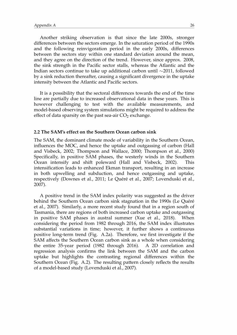
FIGURE A.2: The relationship between the SAM index and the CO2 flux anomaly from January 1982through 2016. (a) Standardized SAM index, smoothed with a 3-month running mean, and the trendline in black. Positive SAM indices are illustrated in red, negative ones in blue. The start of thereinvigoration (Jan 2002) and the most recent period (Jan 2012) are marked with thin vertical blacklines. (a) The correlation coefficients between the sea-air CO2 flux anomaly [mol m−2 yr−1] and thesmoothed, standardized SAM index. Coefficients with significance < 95% are hatched. (c) The slopeof the regression fit between the sea-air CO2 flux anomalies [mol m−2 yr−1] and the standardizedSAM index. As the SAM index is standardized to have a mean of 0 and a standard deviation of 1,(c) illustrates the change in the CO2 flux [mol m−2 yr−1] per standard deviation of the SAM. (b-c)The mean positions of the PF and the STF are illustrated as thin black lines, the three Southern Ocean

sectors are delimited by dashed black lines, and coastal areas are masked white.

In agreement with that study (Lovenduski et al., 2007), positive SAMphases correlate with anomalous outgassing in the region between ∼50◦Sand ∼65◦S, with the exception of the Atlantic sector (Fig. A.2b), potentiallyillustrating the recently suggested zonal SAM asymmetry (Fogt et al., 2012;Sallée et al., 2010). However, we find that for most of the remainingSouthern Ocean, the CO2 flux correlates negatively with the SAM index;here, positive SAM phases are linked to increased uptake. The generalpicture is comprised of alternating zonal bands with positive and negativecorrelations. However, the pattern in the Atlantic sector is approximatelyopposite to the Pacific sector south of ∼45◦S.

Regionally, the link between the SAM and the air-sea exchange of CO2derived from mapped shipboard observations is evident. Just north of thePF in the Pacific sector, anomalous outgassing of approx. 0.5 mol m−2 yr−1

occurs per standard deviation of the SAM (Fig. A.2c). Conversely, south ofthe PF in the Atlantic sector, anomalous carbon uptake of ∼0.4 mol m−2

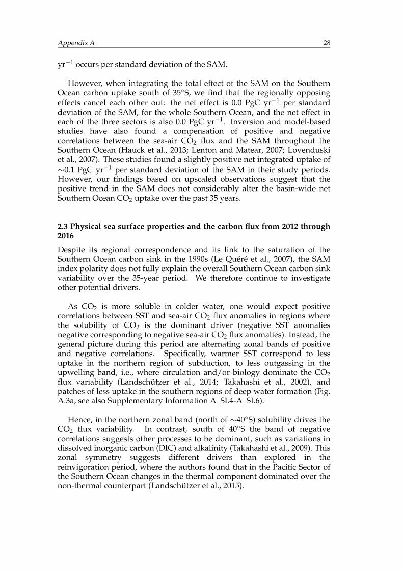
Appendix A 28

yr−1 occurs per standard deviation of the SAM.

However, when integrating the total effect of the SAM on the SouthernOcean carbon uptake south of 35◦S, we find that the regionally opposingeffects cancel each other out: the net effect is 0.0 PgC yr−1 per standarddeviation of the SAM, for the whole Southern Ocean, and the net effect ineach of the three sectors is also 0.0 PgC yr−1. Inversion and model-basedstudies have also found a compensation of positive and negativecorrelations between the sea-air CO2 flux and the SAM throughout theSouthern Ocean (Hauck et al., 2013; Lenton and Matear, 2007; Lovenduskiet al., 2007). These studies found a slightly positive net integrated uptake of∼0.1 PgC yr−1 per standard deviation of the SAM in their study periods.However, our findings based on upscaled observations suggest that thepositive trend in the SAM does not considerably alter the basin-wide netSouthern Ocean CO2 uptake over the past 35 years.

2.3 Physical sea surface properties and the carbon flux from 2012 through2016

Despite its regional correspondence and its link to the saturation of theSouthern Ocean carbon sink in the 1990s (Le Quéré et al., 2007), the SAMindex polarity does not fully explain the overall Southern Ocean carbon sinkvariability over the 35-year period. We therefore continue to investigateother potential drivers.

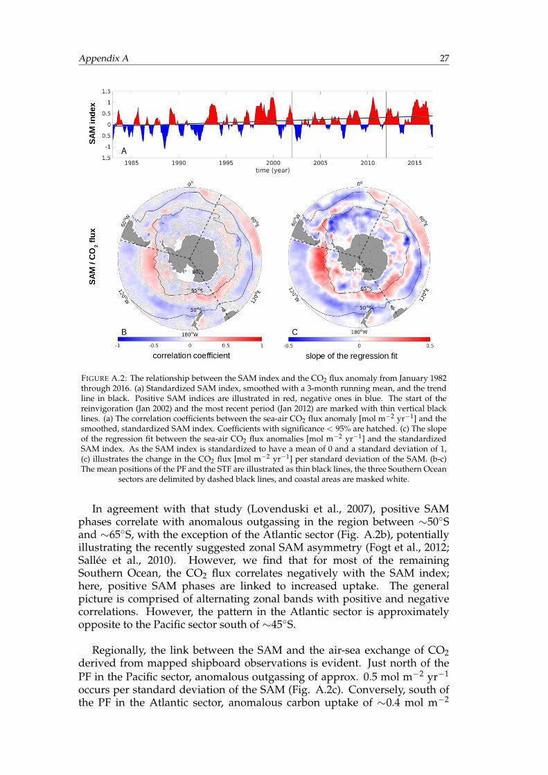
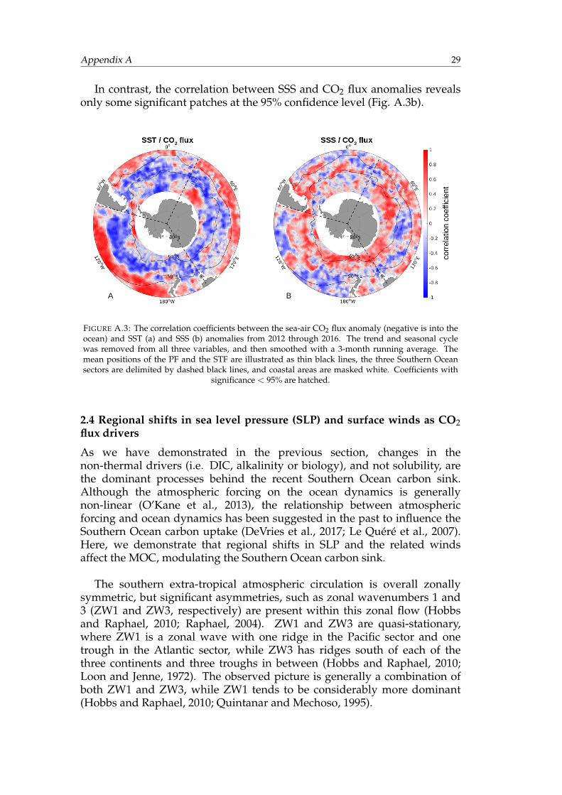
As CO2 is more soluble in colder water, one would expect positivecorrelations between SST and sea-air CO2 flux anomalies in regions wherethe solubility of CO2 is the dominant driver (negative SST anomaliesnegative corresponding to negative sea-air CO2 flux anomalies). Instead, thegeneral picture during this period are alternating zonal bands of positiveand negative correlations. Specifically, warmer SST correspond to lessuptake in the northern region of subduction, to less outgassing in theupwelling band, i.e., where circulation and/or biology dominate the CO2flux variability (Landschützer et al., 2014; Takahashi et al., 2002), andpatches of less uptake in the southern regions of deep water formation (Fig.A.3a, see also Supplementary Information A_SI.4-A_SI.6).

Hence, in the northern zonal band (north of ∼40◦S) solubility drives theCO2 flux variability. In contrast, south of 40◦S the band of negativecorrelations suggests other processes to be dominant, such as variations indissolved inorganic carbon (DIC) and alkalinity (Takahashi et al., 2009). Thiszonal symmetry suggests different drivers than explored in thereinvigoration period, where the authors found that in the Pacific Sector ofthe Southern Ocean changes in the thermal component dominated over thenon-thermal counterpart (Landschützer et al., 2015).

Appendix A 29

In contrast, the correlation between SSS and CO2 flux anomalies revealsonly some significant patches at the 95% confidence level (Fig. A.3b).

FIGURE A.3: The correlation coefficients between the sea-air CO2 flux anomaly (negative is into theocean) and SST (a) and SSS (b) anomalies from 2012 through 2016. The trend and seasonal cyclewas removed from all three variables, and then smoothed with a 3-month running average. Themean positions of the PF and the STF are illustrated as thin black lines, the three Southern Oceansectors are delimited by dashed black lines, and coastal areas are masked white. Coefficients with

significance < 95% are hatched.

2.4 Regional shifts in sea level pressure (SLP) and surface winds as CO2flux drivers

As we have demonstrated in the previous section, changes in thenon-thermal drivers (i.e. DIC, alkalinity or biology), and not solubility, arethe dominant processes behind the recent Southern Ocean carbon sink.Although the atmospheric forcing on the ocean dynamics is generallynon-linear (O’Kane et al., 2013), the relationship between atmosphericforcing and ocean dynamics has been suggested in the past to influence theSouthern Ocean carbon uptake (DeVries et al., 2017; Le Quéré et al., 2007).Here, we demonstrate that regional shifts in SLP and the related windsaffect the MOC, modulating the Southern Ocean carbon sink.

The southern extra-tropical atmospheric circulation is overall zonallysymmetric, but significant asymmetries, such as zonal wavenumbers 1 and3 (ZW1 and ZW3, respectively) are present within this zonal flow (Hobbsand Raphael, 2010; Raphael, 2004). ZW1 and ZW3 are quasi-stationary,where ZW1 is a zonal wave with one ridge in the Pacific sector and onetrough in the Atlantic sector, while ZW3 has ridges south of each of thethree continents and three troughs in between (Hobbs and Raphael, 2010;Loon and Jenne, 1972). The observed picture is generally a combination ofboth ZW1 and ZW3, while ZW1 tends to be considerably more dominant(Hobbs and Raphael, 2010; Quintanar and Mechoso, 1995).

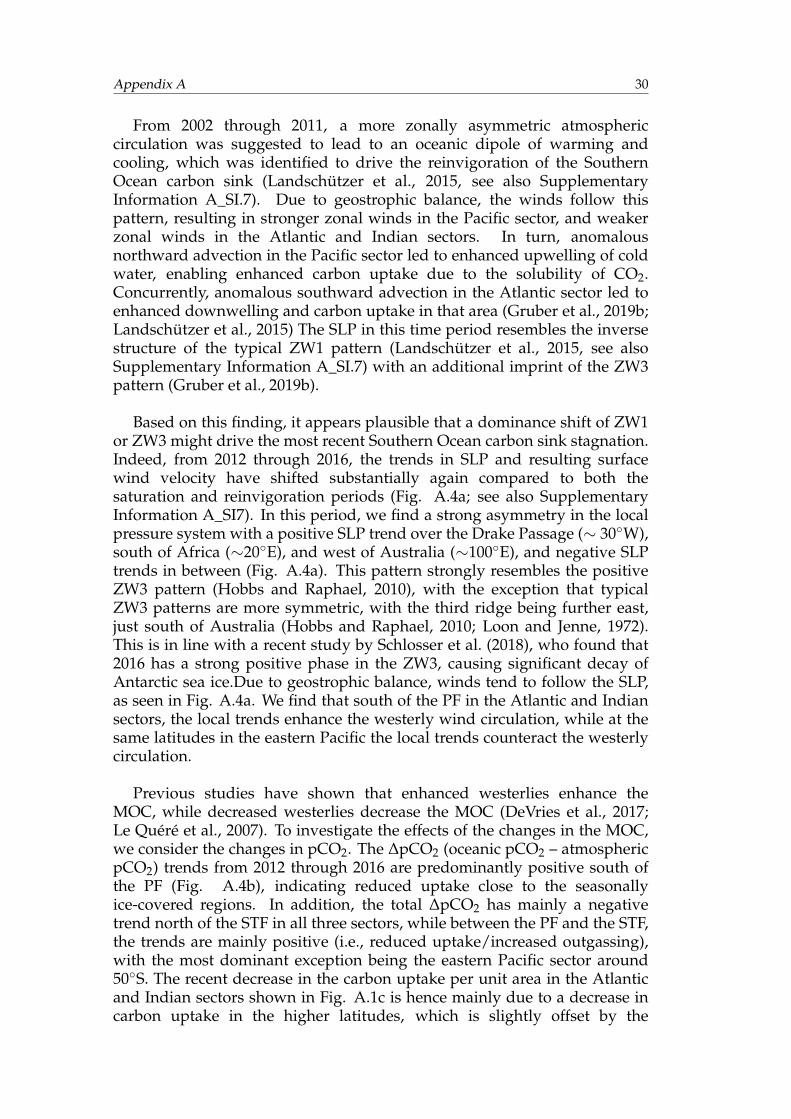
Appendix A 30

From 2002 through 2011, a more zonally asymmetric atmosphericcirculation was suggested to lead to an oceanic dipole of warming andcooling, which was identified to drive the reinvigoration of the SouthernOcean carbon sink (Landschützer et al., 2015, see also SupplementaryInformation A_SI.7). Due to geostrophic balance, the winds follow thispattern, resulting in stronger zonal winds in the Pacific sector, and weakerzonal winds in the Atlantic and Indian sectors. In turn, anomalousnorthward advection in the Pacific sector led to enhanced upwelling of coldwater, enabling enhanced carbon uptake due to the solubility of CO2.Concurrently, anomalous southward advection in the Atlantic sector led toenhanced downwelling and carbon uptake in that area (Gruber et al., 2019b;Landschützer et al., 2015) The SLP in this time period resembles the inversestructure of the typical ZW1 pattern (Landschützer et al., 2015, see alsoSupplementary Information A_SI.7) with an additional imprint of the ZW3pattern (Gruber et al., 2019b).

Based on this finding, it appears plausible that a dominance shift of ZW1or ZW3 might drive the most recent Southern Ocean carbon sink stagnation.Indeed, from 2012 through 2016, the trends in SLP and resulting surfacewind velocity have shifted substantially again compared to both thesaturation and reinvigoration periods (Fig. A.4a; see also SupplementaryInformation A_SI7). In this period, we find a strong asymmetry in the localpressure system with a positive SLP trend over the Drake Passage (∼ 30◦W),south of Africa (∼20◦E), and west of Australia (∼100◦E), and negative SLPtrends in between (Fig. A.4a). This pattern strongly resembles the positiveZW3 pattern (Hobbs and Raphael, 2010), with the exception that typicalZW3 patterns are more symmetric, with the third ridge being further east,just south of Australia (Hobbs and Raphael, 2010; Loon and Jenne, 1972).This is in line with a recent study by Schlosser et al. (2018), who found that2016 has a strong positive phase in the ZW3, causing significant decay ofAntarctic sea ice.Due to geostrophic balance, winds tend to follow the SLP,as seen in Fig. A.4a. We find that south of the PF in the Atlantic and Indiansectors, the local trends enhance the westerly wind circulation, while at thesame latitudes in the eastern Pacific the local trends counteract the westerlycirculation.

Previous studies have shown that enhanced westerlies enhance theMOC, while decreased westerlies decrease the MOC (DeVries et al., 2017;Le Quéré et al., 2007). To investigate the effects of the changes in the MOC,we consider the changes in pCO2. The ∆pCO2 (oceanic pCO2 – atmosphericpCO2) trends from 2012 through 2016 are predominantly positive south ofthe PF (Fig. A.4b), indicating reduced uptake close to the seasonallyice-covered regions. In addition, the total ∆pCO2 has mainly a negativetrend north of the STF in all three sectors, while between the PF and the STF,the trends are mainly positive (i.e., reduced uptake/increased outgassing),with the most dominant exception being the eastern Pacific sector around50◦S. The recent decrease in the carbon uptake per unit area in the Atlanticand Indian sectors shown in Fig. A.1c is hence mainly due to a decrease incarbon uptake in the higher latitudes, which is slightly offset by the

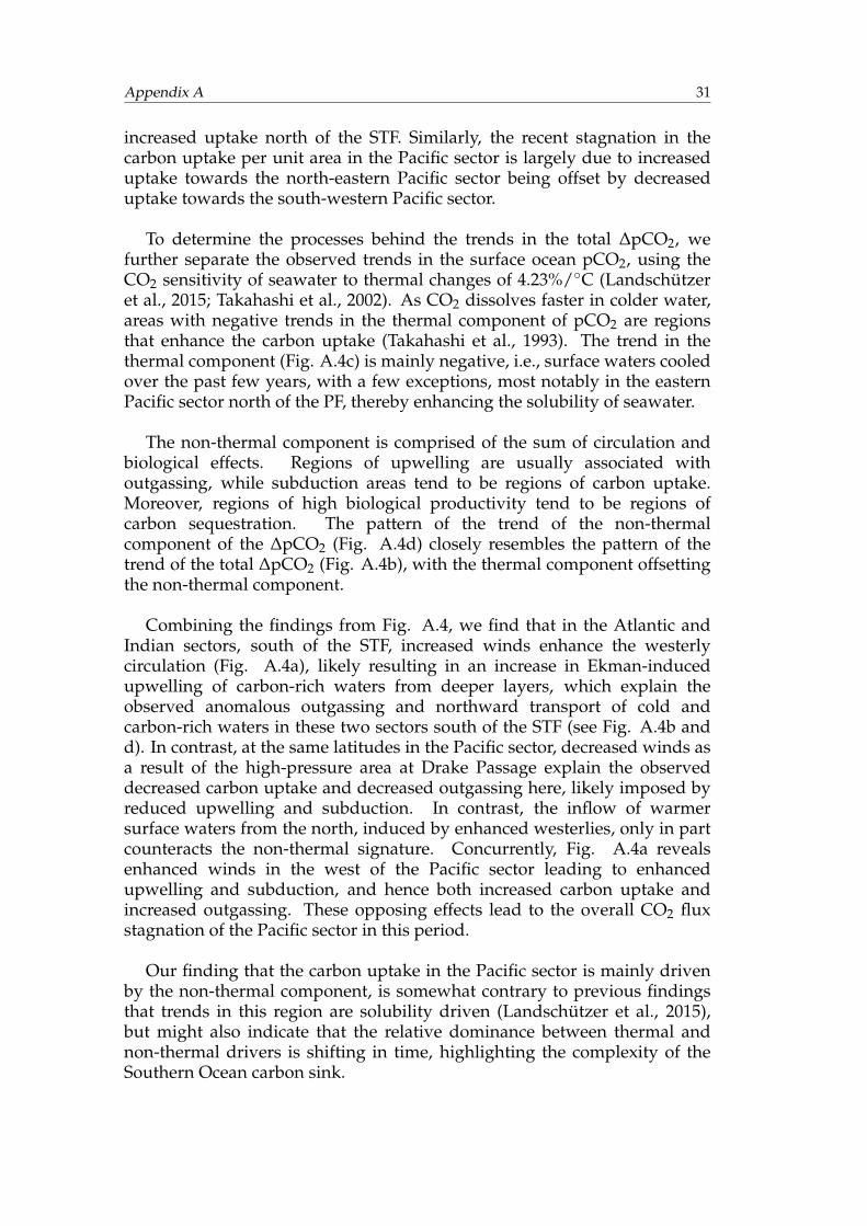
Appendix A 31

increased uptake north of the STF. Similarly, the recent stagnation in thecarbon uptake per unit area in the Pacific sector is largely due to increaseduptake towards the north-eastern Pacific sector being offset by decreaseduptake towards the south-western Pacific sector.

To determine the processes behind the trends in the total ∆pCO2, wefurther separate the observed trends in the surface ocean pCO2, using theCO2 sensitivity of seawater to thermal changes of 4.23%/◦C (Landschützeret al., 2015; Takahashi et al., 2002). As CO2 dissolves faster in colder water,areas with negative trends in the thermal component of pCO2 are regionsthat enhance the carbon uptake (Takahashi et al., 1993). The trend in thethermal component (Fig. A.4c) is mainly negative, i.e., surface waters cooledover the past few years, with a few exceptions, most notably in the easternPacific sector north of the PF, thereby enhancing the solubility of seawater.

The non-thermal component is comprised of the sum of circulation andbiological effects. Regions of upwelling are usually associated withoutgassing, while subduction areas tend to be regions of carbon uptake.Moreover, regions of high biological productivity tend to be regions ofcarbon sequestration. The pattern of the trend of the non-thermalcomponent of the ∆pCO2 (Fig. A.4d) closely resembles the pattern of thetrend of the total ∆pCO2 (Fig. A.4b), with the thermal component offsettingthe non-thermal component.

Combining the findings from Fig. A.4, we find that in the Atlantic andIndian sectors, south of the STF, increased winds enhance the westerlycirculation (Fig. A.4a), likely resulting in an increase in Ekman-inducedupwelling of carbon-rich waters from deeper layers, which explain theobserved anomalous outgassing and northward transport of cold andcarbon-rich waters in these two sectors south of the STF (see Fig. A.4b andd). In contrast, at the same latitudes in the Pacific sector, decreased winds asa result of the high-pressure area at Drake Passage explain the observeddecreased carbon uptake and decreased outgassing here, likely imposed byreduced upwelling and subduction. In contrast, the inflow of warmersurface waters from the north, induced by enhanced westerlies, only in partcounteracts the non-thermal signature. Concurrently, Fig. A.4a revealsenhanced winds in the west of the Pacific sector leading to enhancedupwelling and subduction, and hence both increased carbon uptake andincreased outgassing. These opposing effects lead to the overall CO2 fluxstagnation of the Pacific sector in this period.

Our finding that the carbon uptake in the Pacific sector is mainly drivenby the non-thermal component, is somewhat contrary to previous findingsthat trends in this region are solubility driven (Landschützer et al., 2015),but might also indicate that the relative dominance between thermal andnon-thermal drivers is shifting in time, highlighting the complexity of theSouthern Ocean carbon sink.

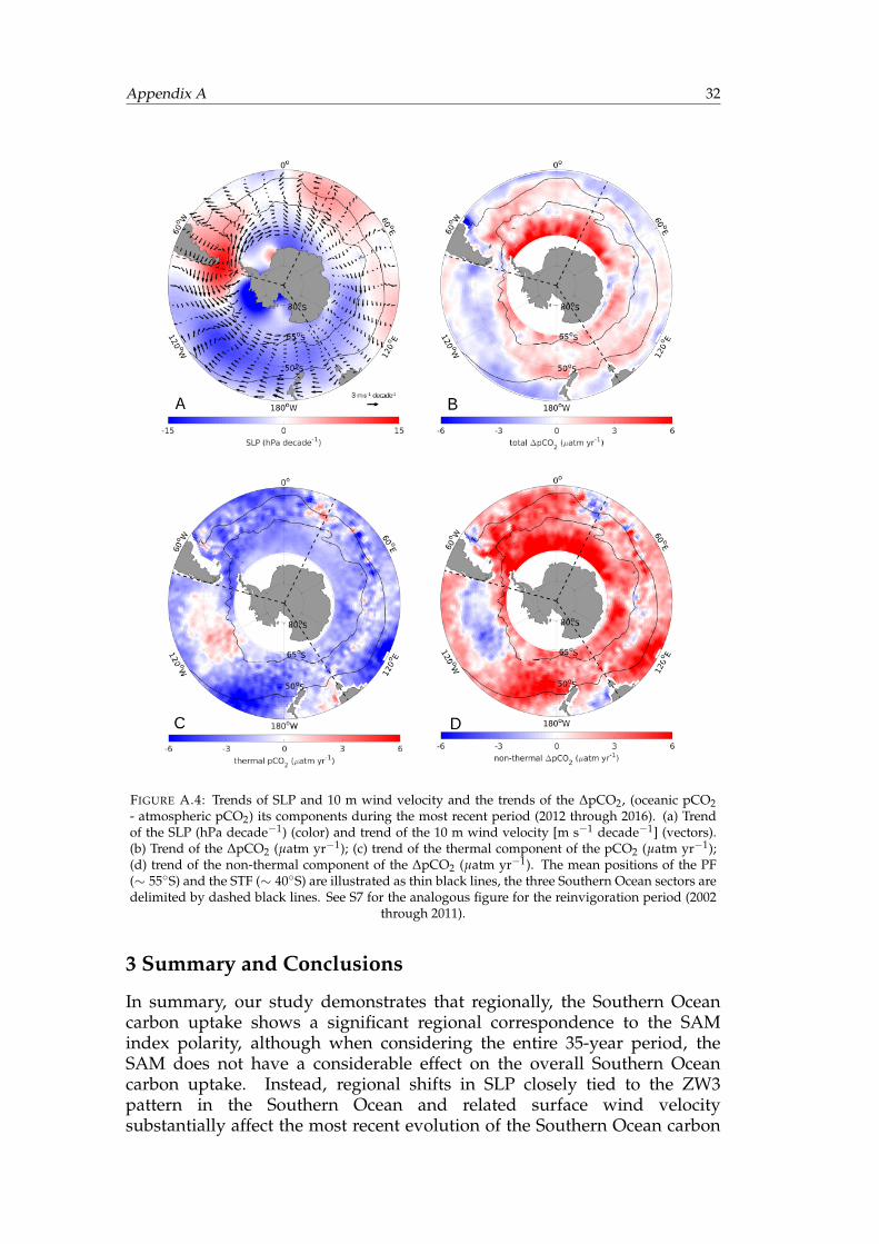
Appendix A 32

FIGURE A.4: Trends of SLP and 10 m wind velocity and the trends of the ∆pCO2, (oceanic pCO2- atmospheric pCO2) its components during the most recent period (2012 through 2016). (a) Trendof the SLP (hPa decade−1) (color) and trend of the 10 m wind velocity [m s−1 decade−1] (vectors).(b) Trend of the ∆pCO2 (µatm yr−1); (c) trend of the thermal component of the pCO2 (µatm yr−1);(d) trend of the non-thermal component of the ∆pCO2 (µatm yr−1). The mean positions of the PF(∼ 55◦S) and the STF (∼ 40◦S) are illustrated as thin black lines, the three Southern Ocean sectors aredelimited by dashed black lines. See S7 for the analogous figure for the reinvigoration period (2002

through 2011).

3 Summary and Conclusions

In summary, our study demonstrates that regionally, the Southern Oceancarbon uptake shows a significant regional correspondence to the SAMindex polarity, although when considering the entire 35-year period, theSAM does not have a considerable effect on the overall Southern Oceancarbon uptake. Instead, regional shifts in SLP closely tied to the ZW3pattern in the Southern Ocean and related surface wind velocitysubstantially affect the most recent evolution of the Southern Ocean carbon

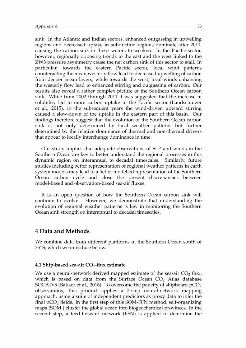
Appendix A 33

sink. In the Atlantic and Indian sectors, enhanced outgassing in upwellingregions and decreased uptake in subduction regions dominate after 2011,causing the carbon sink in these sectors to weaken. In the Pacific sector,however, regionally opposing trends to the east and the west linked to theZW3 pressure asymmetry cause the net carbon sink of this sector to stall. Inparticular, towards the eastern Pacific sector, local wind patternscounteracting the mean westerly flow lead to decreased upwelling of carbonfrom deeper ocean layers, while towards the west, local winds enhancingthe westerly flow lead to enhanced stirring and outgassing of carbon. Ourresults also reveal a rather complex picture of the Southern Ocean carbonsink. While from 2002 through 2011 it was suggested that the increase insolubility led to more carbon uptake in the Pacific sector (Landschützeret al., 2015), in the subsequent years the wind-driven upward stirringcaused a slow-down of the uptake in the eastern part of this basin. Ourfindings therefore suggest that the evolution of the Southern Ocean carbonsink is not only determined by local weather patterns but furtherdetermined by the relative dominance of thermal and non-thermal driversthat appear to locally interchange dominance in time.

Our study implies that adequate observations of SLP and winds in theSouthern Ocean are key to better understand the regional processes in thisdynamic region on interannual to decadal timescales. Similarly, futurestudies including better representation of regional weather patterns in earthsystem models may lead to a better modelled representation of the SouthernOcean carbon cycle and close the present discrepancies betweenmodel-based and observation-based sea-air fluxes.

It is an open question of how the Southern Ocean carbon sink willcontinue to evolve. However, we demonstrate that understanding theevolution of regional weather patterns is key in monitoring the SouthernOcean sink strength on interannual to decadal timescales.

4 Data and Methods

We combine data from different platforms in the Southern Ocean south of35◦S, which we introduce below.

4.1 Ship-based sea-air CO2-flux estimate

We use a neural-network derived mapped estimate of the sea-air CO2 flux,which is based on data from the Surface Ocean CO2 Atlas databaseSOCATv5 (Bakker et al., 2016). To overcome the paucity of shipboard pCO2observations, this product applies a 2-step neural-network mappingapproach, using a suite of independent predictors as proxy data to infer thefinal pCO2 fields. In the first step of this SOM-FFN method, self-organizingmaps (SOM ) cluster the global ocean into biogeochemical provinces. In thesecond step, a feed-forward network (FFN) is applied to determine the

Appendix A 34

statistical relationships between the SOCATv5 data (Bakker et al., 2016) andproxy parameters within the provinces to then estimate the pCO2. Lastly,the sea-air CO2 flux is computed using a bulk flux formulation, wherepositive values indicate outgassing, and negative values indicate oceanicuptake of CO2. The gas transfer is computed using a quadratic winddependence (Wanninkhof, 1992) based on ERA-interim wind speeds (Deeet al., 2011). The gas transfer coefficient is then scaled so that the meantransfer velocity of 16 cm hr-1 matches a recent estimate by Wanninkhofet al. (2013) For more information on this method see Landschützer et al.(2013) and for a discussion on the robustness of this data estimate, see S2.This mapped estimate is on a 1◦x 1◦ monthly grid, originally created from1982 through 2011 (Landschützer et al., 2014; Landschützer et al., 2016). Weextend it by five additional years until December 2016. We compute the CO2flux anomalies by removing the climatological seasonal cycle and smooththe remaining high-frequency variability using a 3-month running mean.

4.2 The SAM index

We use the SAM index by Marshall (2003), which is based on the observedpressure difference between six stations at 40◦S and 65◦S. We standardisethe index by subtracting the mean and dividing it by the standard deviationover the time period (1958 to 2017), following Lovenduski et al. (2007). Wethen smooth the standardised index with a 3-month running mean in orderto be able to analyse the interannual signal of the SAM, following Lentonand Matear (2007). Although some studies do not smooth the SAM index atall, others smooth with a running mean of 8 or 12 months (Hauck et al.,2013; Lenton and Matear, 2007; Lovenduski et al., 2007). We tested differenthigh-pass and low-pass filters and found that the 3-month running meancan represent the interannual variability of the SAM index withoutremoving too much of the signal.

4.3 Argo float-based SST and SSS

Argo floats are autonomous profiling floats that measure seawaterproperties in the water column (http://www.argo.ucsd.edu/). As such,they fill large observational gaps in the ocean, especially in historicallyunder-sampled regions, such as the Southern Ocean. The Roemmich andGilson (2009) Argo-based product provides optimally interpolated data oftemperature and salinity of the top 2000 m on a monthly 1◦x 1◦ grid. Due tothe relatively high spatiotemporal density of floats compared to ship data,this data set is of high confidence and provides reliable in-situ data. We usethe shallowest value at 2.5 m of the temperature and salinity for the SST andSSS respectively from January 2004 until December 2016 (i.e., 13 years ofdata). Based on the data availability of this product, the analysis of the seasurface properties only extends until 65◦S. It would be interesting to analysethe region south of 65◦S as well, as this is a region of deep water formationand hence subduction. However, as this region is partially ice-covered, thereare few Argo profiles with good quality control flags, which results in data

Appendix A 35

with lower confidence than the gridded Argo-based data we use in thisstudy. It has to be left for future analyses to investigate the relationshipbetween the physical sea surface properties and the carbon sink in thisregion. As for the sea-air CO2 flux, we compute anomalies by removing theclimatological seasonal cycle and we smooth remaining high-frequencyvariability using a 3-month running mean.

4.4 SLP and surface wind velocity

To analyse how the SLP and related wind velocity affects the SouthernOcean carbon uptake, we use reanalysis data between January 2004 andDecember 2016. For the SLP, we used the NCEP/NCAR Reanalysis monthlymean data (www.esrl.noaa.gov/psd/data/gridded/data.ncep.reanalysis.surface.html), and for the wind velocity, we use the monthly mean zonaland meridional 10 m wind velocity components from Era Interim (http://apps.ecmwf.int/datasets/data/interim-full-daily/levtype=sfc/).

4.5 Separation into thermal and non-thermal components and ∆pCO2

Following Takahashi et al. (2002), we separate the thermal and non-thermalcomponents of the pCO2 at each grid point using Eq. A.1 and A.2:

non − thermal = pCO2 · EXP(0.0423 · (sstmean − sst)) (A.1)

thermal = pCO2mean · EXP(0.0423 · (sst − sstmean)) (A.2)

where at each grid point, pCO2 is the oceanic pCO2 at a given point in time,pCO2mean is the mean pCO2 over the whole time period, sst is the SST at thegiven point in time, and sstmean is the mean SST of the whole time period.Following Landschützer et al. (2015), we compute ∆pCO2 by subtracting theatmospheric pCO2 at each grid point from the oceanic pCO2 at the samegrid point. We obtain atmospheric xCO2 from the NOAA marine boundarylayer reference product (https://www.esrl.noaa.gov/gmd/ccgg/mbl/).From this, we calculate atmospheric pCO2 as outlined in Landschützer et al.(2013) using the NCEP sea level pressure (Kalnay et al., 1996) and the watervapour correction by Dickson et al. (2007).

4.6 Ocean sectors and position of fronts

To analyse sectoral differences within the Southern Ocean, we define theAtlantic sector from 70◦W to 20◦E, the Indian sector from 20◦E to 145◦E, andthe Pacific sector from 145◦E to 70◦W (see Fig. A.1a). We chose to divide theSouthern Ocean into these sectors and not, e.g., into water masses, becausethe sectors are separated by fixed lines, while other ways of dividing theocean are dynamic and not straight-forward. In addition, similar processesare at play within each of the sectors. Furthermore, several fronts separatethe Southern Ocean and divide it into inter-frontal zones with uniquebiogeochemical and physical properties (e.g., Roemmich and Gilson (2009)).For our analysis and discussion, we use the Subtropical Front (STF) at

Appendix A 36

∼40◦S and the Polar Front (PF) at ∼55◦S as defined by Orsi et al., 1995 (seeFig. A.1a). Although we use the mean position of the fronts, the positions ofthe fronts are not static as they change their position on time scales fromintra- to interannual (Trull et al., 2001).

37

B Seasonal Carbon Dynamics in the Global Ocean based ona Neural-Network Mapping of Observations

Keppler, Lydia1,2, Peter Landschützer1, Nicolas Gruber3, Siv Kari Lauvset4,Irene Stemmler1

1 Max-Planck-Institute for Meteorology (MPI-M), Hamburg, Germany.2 International Max Planck Research School on Earth System Modelling(IMPRS-ESM), Hamburg, Germany.3 Environmental Physics, Institute of Biogeochemistry and PollutantDynamics, ETH Zurich, Switzerland4 NORCE Norwegian Research Centre, Bjerknes Centre for ClimateResearch, Bergen, Norway

Paper status at the time of the submission of this thesis:In Review at the Journal of Global Biogeochemical Cycles

Data availability:The data product created during this study is freely available to the public(will be submitted to NCEI OCADS after publication of this paper).

Supplementary Information accompanies this paper at the end of thisAppendix.

Contributions: L.K. and P.L. designed the research; L.K. performed the research;L.K. wrote the draft manuscript; all authors contributed to the discussion of theresults and the manuscript at all stages.

Appendix B 38

Abstract

The seasonal cycle represents one of the largest perturbations of the naturalcarbon cycle in the ocean, yet the global seasonal pattern of dissolvedinorganic carbon (DIC) is not well established. Here, we present the firstglobal monthly climatology of oceanic DIC extending from the surface to2000 m, obtained by a 2-step neural network method and DICmeasurements from the GLODAPv2.2019 data product. Tests with syntheticdata from an ocean biogeochemistry model and with independentobservations demonstrate that the method successfully captures thespatio-temporal variability of DIC with an average root mean squared errorof ∼20 µmol kg−1. We find the largest amplitudes of the seasonal cycle ofsurface DIC in the northern high latitude Pacific (∼30 to >50 µmol kg−1).Surface maxima tend to occur in hemispheric spring and minima in latesummer, driven by the input of DIC into the upper ocean by mixing duringwinter/early spring, and the subsequent biological draw-down of DIC insummer. This seasonal pattern extends to a nodal depth of <50 m in thetropics and several hundred meters in the subtropics, below which theseasonal cycle has the opposite phase, although with a smaller amplitude.From the carbon draw-down, we estimate the hemispheric summer netcommunity production (NCP) from the surface to the base of the euphoticzone at global scale. We find a global mean summer NCP of ∼1.4±0.2 mol Cm−2 (∼6.1±0.9 PgC) with the highest production rates in the North Atlantic(up to ∼5 mol C m−2).

1 Introduction

The vast majority of the dissolved inorganic carbon (DIC) that exists in theocean is part of the natural carbon cycle. This pool of roughly 36,000 PgC (1PgC = 1015 g carbon) contains about 90% of the total amount of carbon inthe ocean, atmosphere, and land biosphere system combined (Ciais et al.,2014). Since the beginning of the industrial revolution, human activities,mostly through the release of anthropogenic carbon dioxide (CO2) from theburning of fossil fuels and land-use change, have perturbed these poolssubstantially. By the year 2007, the ocean DIC pool had grown by 152±20PgC relative to the year 1800 through the uptake of this anthropogenic CO2from the atmosphere (Gruber et al., 2019b). The current oceanic net uptakerate of 2.5±0.6 PgC yr−1 constitutes approximately 23% of theanthropogenic CO2 emissions on an annual basis, thereby highlighting thecrucial role of the ocean in ameliorating one of the key drivers of climatechange (Friedlingstein et al., 2019; Le Quéré et al., 2018). Thus, it is notsurprising that nearly all studies in the last four decades investigatingchanges in the interior distribution of DIC have focused on this long-termanthropogenic perturbation of oceanic DIC (Brewer, 1978; Chen andMillero, 1979; Gruber et al., 1996; Sabine and Tanhua, 2010).

In contrast, changes in the natural carbon cycle, and especially thosechanges in oceanic DIC occurring on seasonal timescales have received

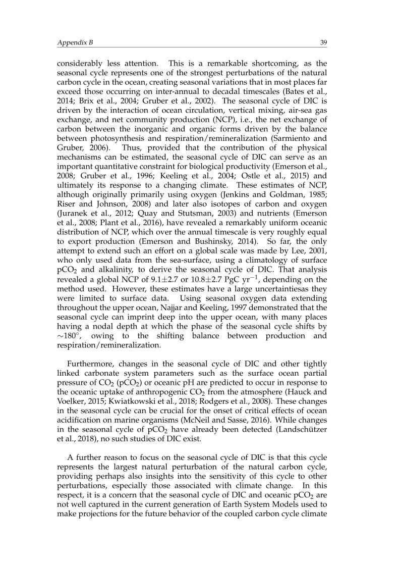
Appendix B 39

considerably less attention. This is a remarkable shortcoming, as theseasonal cycle represents one of the strongest perturbations of the naturalcarbon cycle in the ocean, creating seasonal variations that in most places farexceed those occurring on inter-annual to decadal timescales (Bates et al.,2014; Brix et al., 2004; Gruber et al., 2002). The seasonal cycle of DIC isdriven by the interaction of ocean circulation, vertical mixing, air-sea gasexchange, and net community production (NCP), i.e., the net exchange ofcarbon between the inorganic and organic forms driven by the balancebetween photosynthesis and respiration/remineralization (Sarmiento andGruber, 2006). Thus, provided that the contribution of the physicalmechanisms can be estimated, the seasonal cycle of DIC can serve as animportant quantitative constraint for biological productivity (Emerson et al.,2008; Gruber et al., 1996; Keeling et al., 2004; Ostle et al., 2015) andultimately its response to a changing climate. These estimates of NCP,although originally primarily using oxygen (Jenkins and Goldman, 1985;Riser and Johnson, 2008) and later also isotopes of carbon and oxygen(Juranek et al., 2012; Quay and Stutsman, 2003) and nutrients (Emersonet al., 2008; Plant et al., 2016), have revealed a remarkably uniform oceanicdistribution of NCP, which over the annual timescale is very roughly equalto export production (Emerson and Bushinsky, 2014). So far, the onlyattempt to extend such an effort on a global scale was made by Lee, 2001,who only used data from the sea-surface, using a climatology of surfacepCO2 and alkalinity, to derive the seasonal cycle of DIC. That analysisrevealed a global NCP of 9.1±2.7 or 10.8±2.7 PgC yr−1, depending on themethod used. However, these estimates have a large uncertaintiesas theywere limited to surface data. Using seasonal oxygen data extendingthroughout the upper ocean, Najjar and Keeling, 1997 demonstrated that theseasonal cycle can imprint deep into the upper ocean, with many placeshaving a nodal depth at which the phase of the seasonal cycle shifts by∼180◦, owing to the shifting balance between production andrespiration/remineralization.

Furthermore, changes in the seasonal cycle of DIC and other tightlylinked carbonate system parameters such as the surface ocean partialpressure of CO2 (pCO2) or oceanic pH are predicted to occur in response tothe oceanic uptake of anthropogenic CO2 from the atmosphere (Hauck andVoelker, 2015; Kwiatkowski et al., 2018; Rodgers et al., 2008). These changesin the seasonal cycle can be crucial for the onset of critical effects of oceanacidification on marine organisms (McNeil and Sasse, 2016). While changesin the seasonal cycle of pCO2 have already been detected (Landschützeret al., 2018), no such studies of DIC exist.

A further reason to focus on the seasonal cycle of DIC is that this cyclerepresents the largest natural perturbation of the natural carbon cycle,providing perhaps also insights into the sensitivity of this cycle to otherperturbations, especially those associated with climate change. In thisrespect, it is a concern that the seasonal cycle of DIC and oceanic pCO2 arenot well captured in the current generation of Earth System Models used tomake projections for the future behavior of the coupled carbon cycle climate

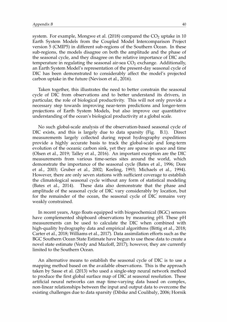
Appendix B 40

system. For example, Mongwe et al. (2018) compared the CO2 uptake in 10Earth System Models from the Coupled Model Intercomparison Projectversion 5 (CMIP5) in different sub-regions of the Southern Ocean. In thesesub-regions, the models disagree on both the amplitude and the phase ofthe seasonal cycle, and they disagree on the relative importance of DIC andtemperature in regulating the seasonal air-sea CO2 exchange. Additionally,an Earth System Model’s representation of the present-day seasonal cycle ofDIC has been demonstrated to considerably affect the model’s projectedcarbon uptake in the future (Nevison et al., 2016).

Taken together, this illustrates the need to better constrain the seasonalcycle of DIC from observations and to better understand its drivers, inparticular, the role of biological productivity. This will not only provide anecessary step towards improving near-term predictions and longer-termprojections of Earth System Models, but also improve our quantitativeunderstanding of the ocean’s biological productivity at a global scale.

No such global-scale analysis of the observation-based seasonal cycle ofDIC exists, and this is largely due to data sparsity (Fig. B.1). Directmeasurements largely collected during repeat hydrography expeditionsprovide a highly accurate basis to track the global-scale and long-termevolution of the oceanic carbon sink, yet they are sparse in space and time(Olsen et al., 2019; Talley et al., 2016). An important exception are the DICmeasurements from various time-series sites around the world, whichdemonstrate the importance of the seasonal cycle (Bates et al., 1996; Doreet al., 2003; Gruber et al., 2002; Keeling, 1993; Michaels et al., 1994).However, there are only seven stations with sufficient coverage to establishthe climatological seasonal cycle without any form of statistical modeling(Bates et al., 2014). These data also demonstrate that the phase andamplitude of the seasonal cycle of DIC vary considerably by location, butfor the remainder of the ocean, the seasonal cycle of DIC remains veryweakly constrained.

In recent years, Argo floats equipped with biogeochemical (BGC) sensorshave complemented shipboard observations by measuring pH. These pHmeasurements can be used to calculate the DIC when combined withhigh-quality hydrography data and empirical algorithms (Bittig et al., 2018;Carter et al., 2018; Williams et al., 2017). Data assimilation efforts such as theBGC Southern Ocean State Estimate have begun to use these data to create anovel state estimate (Verdy and Mazloff, 2017); however, they are currentlylimited to the Southern Ocean.

An alternative means to establish the seasonal cycle of DIC is to use amapping method based on the available observations. This is the approachtaken by Sasse et al. (2013) who used a single-step neural network methodto produce the first global surface map of DIC at seasonal resolution. Theseartificial neural networks can map time-varying data based on complex,non-linear relationships between the input and output data to overcome theexisting challenges due to data sparsity (Dibike and Coulibaly, 2006; Hornik

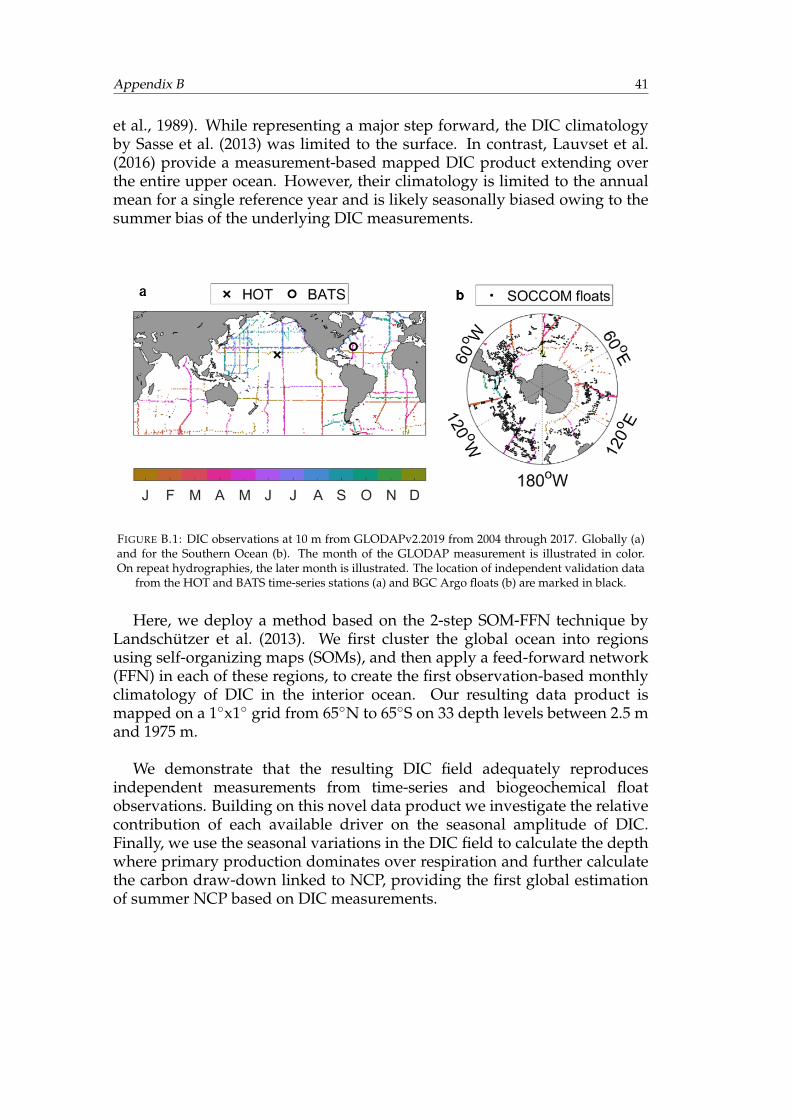
Appendix B 41

et al., 1989). While representing a major step forward, the DIC climatologyby Sasse et al. (2013) was limited to the surface. In contrast, Lauvset et al.(2016) provide a measurement-based mapped DIC product extending overthe entire upper ocean. However, their climatology is limited to the annualmean for a single reference year and is likely seasonally biased owing to thesummer bias of the underlying DIC measurements.

FIGURE B.1: DIC observations at 10 m from GLODAPv2.2019 from 2004 through 2017. Globally (a)and for the Southern Ocean (b). The month of the GLODAP measurement is illustrated in color.On repeat hydrographies, the later month is illustrated. The location of independent validation data

from the HOT and BATS time-series stations (a) and BGC Argo floats (b) are marked in black.

Here, we deploy a method based on the 2-step SOM-FFN technique byLandschützer et al. (2013). We first cluster the global ocean into regionsusing self-organizing maps (SOMs), and then apply a feed-forward network(FFN) in each of these regions, to create the first observation-based monthlyclimatology of DIC in the interior ocean. Our resulting data product ismapped on a 1◦x1◦ grid from 65◦N to 65◦S on 33 depth levels between 2.5 mand 1975 m.

We demonstrate that the resulting DIC field adequately reproducesindependent measurements from time-series and biogeochemical floatobservations. Building on this novel data product we investigate the relativecontribution of each available driver on the seasonal amplitude of DIC.Finally, we use the seasonal variations in the DIC field to calculate the depthwhere primary production dominates over respiration and further calculatethe carbon draw-down linked to NCP, providing the first global estimationof summer NCP based on DIC measurements.

Appendix B 42

2 Data and Methods

2.1 Reconstructing global mapped fields of DIC using SOM-FFN

We use the 2-step SOM-FFN approach by Landschützer et al. (2013) with theDIC observations from GLODAPv2.2019 throughout the upper 2000 m. TheSOM-FFN method first clusters the global ocean into regions of similarbiogeochemical properties using SOMs. In a second step, it runs an FFN ineach cluster to establish the statistical relationship between the measuredDIC and a set of physical and biogeochemical predictors. Next, global fieldsof these predictors are used to project the statistically modeled DIC into theocean for each month and depth. This section provides a summary of theSOM-FFN approach and some of the adjustments made from the approachdescribed by Landschützer et al. (2013). A more detailed description of ourmethod and data can be found in the Supplementary Information B_S1 -B_S4.

Here, we apply and extend the SOM-FFN method using DIC as the targetvariable for the mapping. We map DIC not only at the sea surface, but alsothroughout the upper water column from the surface until ∼2000 m. We usethe DIC measurements from GLODAPv2.2019 from 2004 through 2017(Olsen et al., 2019) as the input for the FFN (Fig. B.1). This temporalrestriction reduces the impact of the long-term trend in DIC, drivenprimarily by the oceanic uptake of anthropogenic CO2 from the atmosphere.The method reconstructs the non-linear best-fit relationship between all ofthe available observations and a set of physical and biogeochemicalpredictor data. These predictor data exist on a global scale, hence thereconstructed relationship can be applied where no observations exist to fillthe data gaps (see Landschützer et al. (2013) and SupplementaryInformation B_S1 - B_S4).

As predictor data, we chose representative proxies for the effect of oceanphysics, chemistry, and biology on the DIC field. We use optimallyinterpolated temperature and salinity fields based on Argo floats (Argo,2019; Roemmich and Gilson, 2009), and optimally interpolated fields ofsilicate, nitrate, and dissolved oxygen from the World Ocean Atlas 2018(Garcia et al., 2019). The predictors have a known interaction with DIC andare available as monthly global mapped fields in the water column. Ouroutput consists of monthly mean fields of DIC based on the period from2004 through 2017, on 33 depth levels between 2.5 m and 1975 m on a 1◦x1◦grid from 65◦N to 65◦S.

2.2 Smoothing and uncertainty within the method

The internal validation of the SOM-FFN method is based on a randomlychosen subsample of the available observations by the network (seeSupplementary Information B_S3). Therefore, the resulting DIC fields varyslightly each time we run the network. To account for potential biases in theseparation between training and validation data, we use a bootstrapping

Appendix B 43

approach and run the SOM-FFN method ten times and take the mean of thisensemble, resulting in a smoother end product than a single ensemblemember. We define the generalization uncertainty within the method as thestandard deviation across this ensemble. The mapped ensemble mean fieldsare further smoothed at each depth level with a scalar function-basedfiltering using the mean of the neighboring three grid cells in each directionexcept depth (month, latitude, and longitude). We estimate the seasonalcycle by applying a non-linear least squares harmonic fit at each grid cell, ateach depth level. Our final neural-network derived estimate of DIC ishereafter called DICNN (Table B.1).

2.3 Test with synthetic data

In addition to validating our method with independent measurements, wetest our method with synthetic data. We take the model field from the oceanbiogeochemistry model HAMOCC (Ilyina et al., 2013; Mauritsen et al.,2019), which was run on a 1.5◦x1.5◦ grid in hindcast mode with historicatmospheric forcing for the Global Carbon Budget 2018 (Le Quéré et al.,2018). We first re-grid the HAMOCC output onto the same grid and formatas the observational predictor and target data (monthly means between 2004through 2017, 33 depth levels between 2.5 m and 1975 m, 1◦x1◦ grid, from65◦N to 65◦S). We call the full model field of DIC in HAMOCC hereafterDICHAMOCC (Table B.1).

To test how well our method reconstructs the full model field, wesubsample DICHAMOCC at the month and location where we have DICobservations in GLODAPv2.2019. We then use the same SOM-FFN set-up(as described in full detail in Supplementary Information B_S1 - B_S3) andrun the method using the same predictors, but from HAMOCC, to estimatethe DIC in HAMOCC (hereafter DICNN.HAMOCC). Finally, we compareDICNN.HAMOCC with DICHAMOCC.

2.4 Test with independent measurements

We further compare our estimate with data from independent time-seriessites that were not fed into the network and have a long enough record toextract the mean seasonality. Although there are many time-series stationsacross the globe (Bates et al., 2014) (See also https://www.nodc.noaa.gov/ocads/oceans/time_series_moorings.html), only a few stations measuredDIC in the upper ocean from 2004 through 2017 and at locations that are notexcluded in our product (i.e., coastal regions and latitudes poleward of 65◦).The time-series stations that fall within our temporal and spatial domainsare the Hawaii Ocean Time-Series (HOT) (Dore et al., 2009) and the BermudaAtlantic Time Series Study (BATS) (Bates et al., 2014).

Appendix B 44

The HOT (http://www.soest.hawaii.edu/HOT_WOCE/ftp.html) andBATS (http://batsftp.bios.edu/BATS/bottle/A_README_BOTTLE.txt)databases consist of physical and BGC ship data. The DIC measurementsthat form a part of these time-series datasets were taken from bottledsea-water samples. The HOT time-series extends from 1988 through 2017for the upper ocean at 22◦45’N, 158◦00’W, north of Hawaii, while the BATStime series extends from 1988 through 2016 at 31◦40’N, 64◦10’W (Fig. B.1a).

For the validation, we compile all DIC measurements from the HOT andBATS databases and only keep the data that overlap with the period fromour study (2004 through 2017). At BATS, while conducting our analysis,data from 2017 were not available, so here the dataset ends in December2016. We then compute a monthly climatology by taking the mean monthlyvalues. While the HOT data extends to 1000 m, at BATS, only a fewobservations exist below 600 m, so here we only use the top 600 m for ourvalidation.

We test DICNN at the 1◦x1◦ grid point closest to the HOT location(hereafter DICNN.HOT) and compare it to the measured DIC at the HOTstation (hereafter DICHOT). We also test how DICHAMOCC at the grid pointclosest to HOT (hereafter DICHAMOCC.HOT) compares to our estimatethereof (hereafter DICNN.HAMOCC.HOT, Table B.1).

Similarly, we test DICNN at the 1◦x1◦ grid point closest to the BATSlocation (hereafter DICNN.BATS) and compare it to the measured DIC at theBATS station (hereafter DICBATS). We then test how DICHAMOCC at the gridpoint closest to BATS (hereafter DICHAMOCC.BATS) compares to our estimatethereof (hereafter DICNN.HAMOCC.BATS, Table B.1).

To test our method in the southern hemisphere, we use data from BGCArgo floats that take measurements as part of the Southern Ocean Carbonand Climate Observation and Modelling project (SOCCOM). We comparethe monthly mean DIC concentration calculated from the SOCCOM floats toour neural-network derived estimate of the DIC concentration at the monthand location of the float measurements (DICNN.SOCCOM). The DIC from theSOCCOM floats is calculated using a combination of pH measurements,total alkalinity estimated using the commonly used LIAR algorithm (Carteret al., 2018), and the CO2SYS analysis tool (Heuven et al., 2011). As theSOCCOM float data is only available after 2014, we compute the monthlyclimatology of DIC from 2014 through 2017 on a 1◦x1◦ grid and linearlyinterpolate the result onto our 33 depth levels (hereafter DICSOCCOM). In thedomain until 65◦S, there are, on average, 160 grid cells with SOCCOM floatsin each month of the year (Fig. B.1b). The data density of the SOCCOMfloats is relatively high, although the period of these observations onlyextends over four years (2014 through 2017). Lastly, we test howDICHAMOCC at the grid points closest to the SOCCOM floats (hereafterDICHAMOCC.SOCCOM) compares to our estimate thereof (hereafterDICNN.HAMOCC.SOCCOM, Table B.1).

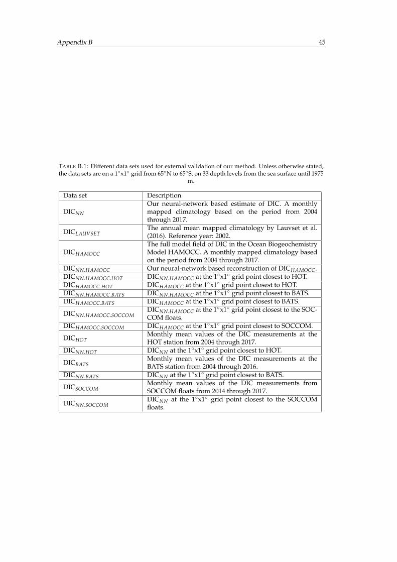
Appendix B 45

TABLE B.1: Different data sets used for external validation of our method. Unless otherwise stated,the data sets are on a 1◦x1◦ grid from 65◦N to 65◦S, on 33 depth levels from the sea surface until 1975

m.

Data set Description

DICNN

Our neural-network based estimate of DIC. A monthlymapped climatology based on the period from 2004through 2017.

DICLAUVSETThe annual mean mapped climatology by Lauvset et al.(2016). Reference year: 2002.

DICHAMOCC

The full model field of DIC in the Ocean BiogeochemistryModel HAMOCC. A monthly mapped climatology basedon the period from 2004 through 2017.

DICNN.HAMOCC Our neural-network based reconstruction of DICHAMOCC.DICNN.HAMOCC.HOT DICNN.HAMOCC at the 1◦x1◦ grid point closest to HOT.DICHAMOCC.HOT DICHAMOCC at the 1◦x1◦ grid point closest to HOT.DICNN.HAMOCC.BATS DICNN.HAMOCC at the 1◦x1◦ grid point closest to BATS.DICHAMOCC.BATS DICHAMOCC at the 1◦x1◦ grid point closest to BATS.

DICNN.HAMOCC.SOCCOMDICNN.HAMOCC at the 1◦x1◦ grid point closest to the SOC-COM floats.

DICHAMOCC.SOCCOM DICHAMOCC at the 1◦x1◦ grid point closest to SOCCOM.

DICHOTMonthly mean values of the DIC measurements at theHOT station from 2004 through 2017.

DICNN.HOT DICNN at the 1◦x1◦ grid point closest to HOT.

DICBATSMonthly mean values of the DIC measurements at theBATS station from 2004 through 2016.

DICNN.BATS DICNN at the 1◦x1◦ grid point closest to BATS.

DICSOCCOMMonthly mean values of the DIC measurements fromSOCCOM floats from 2014 through 2017.

DICNN.SOCCOMDICNN at the 1◦x1◦ grid point closest to the SOCCOMfloats.

Appendix B 46

2.5 Seasonal response function

To investigate how each of the predictors contributes to the seasonalchanges in DIC, we compute the seasonal response function for each of thepredictors. We use an approach similar to the “profile method” described inGevrey et al. (2003), which is commonly used in sensitivity analyses todetermine how changes in the predictors affect the target data in a neuralnetwork. In the profile method, the network is trained as usual (seeSupplementary Information B_S3), and in the simulation step, one predictoris consecutively varied while holding the remaining predictors constant. Aswe are interested in the seasonal response in different regions, we use asimilar approach to the profile method, but we only hold the timedimension constant, while varying in space.

Our method works as follows: We first calculate DICbase by training thenetwork as usual and then apply the network while keeping all predictorsconstant in time (i.e., using the time-mean at each grid cell). Next, wesimulate the network again consecutively for each predictor, while keepingall of the predictors except the predictor under evaluation constant in time.For example, we calculate DICtemperature by simulating the network with allof the predictors kept constant in time, except temperature. Lastly, for eachpredictor, we calculate ∆DICinput by subtracting the DICinput of thatpredictor from the DICbase; for example, for temperature: ∆DICtemperature =DICbase - DICtemperature. We repeat our bootstrapping approach bysimulating these ten times to calculate the mean response over theensemble.

2.6 Nodal depth and summer NCP

To investigate the effect of primary production on the seasonal cycle of DIC,we first compute the nodal depth. Above and below the nodal depth, thephase of the seasonal cycle of DIC differs, due to the opposing effects ofprimary production near the surface and remineralization below. Wedetermine the nodal depth as the depth where the amplitude of the seasonalcycle of DIC is minimal, while it increases both upward and downward ofthe nodal depth.

To determine the summer NCP, we solve the following diagnosticequation following Gruber et al. (1998) and Keeling et al. (2004) (Eq. B.1):∫

NCPdz =∫ DICnorm

dtdz + Fair.sea − Fdi f f − Fentr + Fhor.div (B.1)

where∫

NCP dz is the NCP between the surface and the base of theeuphotic zone,

∫ DICnormdt dz is the change in time of the integrated salinity

normalized DIC from the surface until the base of the euphotic zone, Fair.seais the integrated air-sea CO2 flux over hemispheric summer, Fdi f f is themean vertical diffusive flux over hemispheric summer, Fentr is the meanentrainment flux over hemispheric summer, and Fhor.div is the horizontal

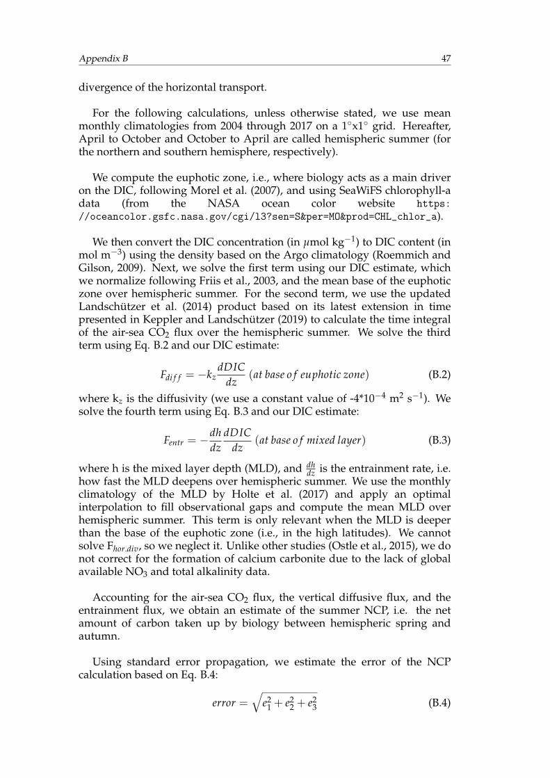
Appendix B 47

divergence of the horizontal transport.

For the following calculations, unless otherwise stated, we use meanmonthly climatologies from 2004 through 2017 on a 1◦x1◦ grid. Hereafter,April to October and October to April are called hemispheric summer (forthe northern and southern hemisphere, respectively).

We compute the euphotic zone, i.e., where biology acts as a main driveron the DIC, following Morel et al. (2007), and using SeaWiFS chlorophyll-adata (from the NASA ocean color website https://oceancolor.gsfc.nasa.gov/cgi/l3?sen=S&per=MO&prod=CHL_chlor_a).

We then convert the DIC concentration (in µmol kg−1) to DIC content (inmol m−3) using the density based on the Argo climatology (Roemmich andGilson, 2009). Next, we solve the first term using our DIC estimate, whichwe normalize following Friis et al., 2003, and the mean base of the euphoticzone over hemispheric summer. For the second term, we use the updatedLandschützer et al. (2014) product based on its latest extension in timepresented in Keppler and Landschützer (2019) to calculate the time integralof the air-sea CO2 flux over the hemispheric summer. We solve the thirdterm using Eq. B.2 and our DIC estimate:

Fdi f f = −kzdDIC

dz(at base o f euphotic zone) (B.2)

where kz is the diffusivity (we use a constant value of -4*10−4 m2 s−1). Wesolve the fourth term using Eq. B.3 and our DIC estimate:

Fentr = −dhdz

dDICdz

(at base o f mixed layer) (B.3)

where h is the mixed layer depth (MLD), and dhdz is the entrainment rate, i.e.

how fast the MLD deepens over hemispheric summer. We use the monthlyclimatology of the MLD by Holte et al. (2017) and apply an optimalinterpolation to fill observational gaps and compute the mean MLD overhemispheric summer. This term is only relevant when the MLD is deeperthan the base of the euphotic zone (i.e., in the high latitudes). We cannotsolve Fhor.div, so we neglect it. Unlike other studies (Ostle et al., 2015), we donot correct for the formation of calcium carbonite due to the lack of globalavailable NO3 and total alkalinity data.

Accounting for the air-sea CO2 flux, the vertical diffusive flux, and theentrainment flux, we obtain an estimate of the summer NCP, i.e. the netamount of carbon taken up by biology between hemispheric spring andautumn.

Using standard error propagation, we estimate the error of the NCPcalculation based on Eq. B.4:

error =√

e21 + e2

2 + e23 (B.4)

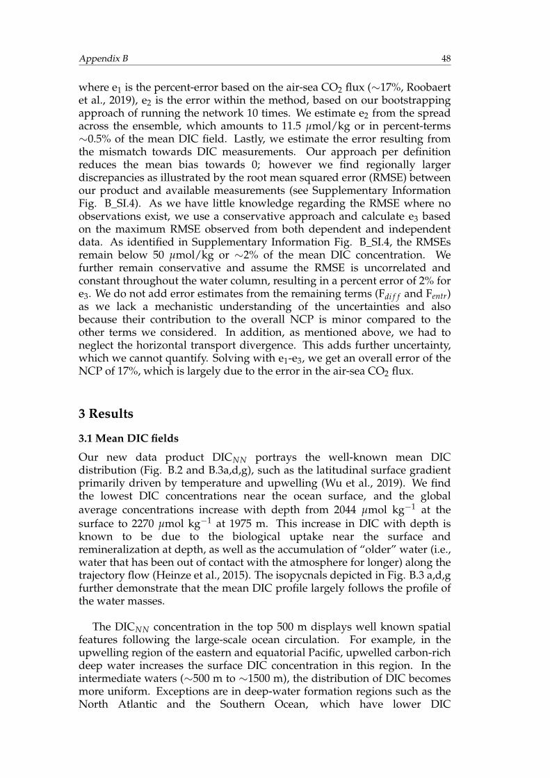
Appendix B 48

where e1 is the percent-error based on the air-sea CO2 flux (∼17%, Roobaertet al., 2019), e2 is the error within the method, based on our bootstrappingapproach of running the network 10 times. We estimate e2 from the spreadacross the ensemble, which amounts to 11.5 µmol/kg or in percent-terms∼0.5% of the mean DIC field. Lastly, we estimate the error resulting fromthe mismatch towards DIC measurements. Our approach per definitionreduces the mean bias towards 0; however we find regionally largerdiscrepancies as illustrated by the root mean squared error (RMSE) betweenour product and available measurements (see Supplementary InformationFig. B_SI.4). As we have little knowledge regarding the RMSE where noobservations exist, we use a conservative approach and calculate e3 basedon the maximum RMSE observed from both dependent and independentdata. As identified in Supplementary Information Fig. B_SI.4, the RMSEsremain below 50 µmol/kg or ∼2% of the mean DIC concentration. Wefurther remain conservative and assume the RMSE is uncorrelated andconstant throughout the water column, resulting in a percent error of 2% fore3. We do not add error estimates from the remaining terms (Fdi f f and Fentr)as we lack a mechanistic understanding of the uncertainties and alsobecause their contribution to the overall NCP is minor compared to theother terms we considered. In addition, as mentioned above, we had toneglect the horizontal transport divergence. This adds further uncertainty,which we cannot quantify. Solving with e1-e3, we get an overall error of theNCP of 17%, which is largely due to the error in the air-sea CO2 flux.

3 Results

3.1 Mean DIC fields

Our new data product DICNN portrays the well-known mean DICdistribution (Fig. B.2 and B.3a,d,g), such as the latitudinal surface gradientprimarily driven by temperature and upwelling (Wu et al., 2019). We findthe lowest DIC concentrations near the ocean surface, and the globalaverage concentrations increase with depth from 2044 µmol kg−1 at thesurface to 2270 µmol kg−1 at 1975 m. This increase in DIC with depth isknown to be due to the biological uptake near the surface andremineralization at depth, as well as the accumulation of “older” water (i.e.,water that has been out of contact with the atmosphere for longer) along thetrajectory flow (Heinze et al., 2015). The isopycnals depicted in Fig. B.3 a,d,gfurther demonstrate that the mean DIC profile largely follows the profile ofthe water masses.

The DICNN concentration in the top 500 m displays well known spatialfeatures following the large-scale ocean circulation. For example, in theupwelling region of the eastern and equatorial Pacific, upwelled carbon-richdeep water increases the surface DIC concentration in this region. In theintermediate waters (∼500 m to ∼1500 m), the distribution of DIC becomesmore uniform. Exceptions are in deep-water formation regions such as theNorth Atlantic and the Southern Ocean, which have lower DIC

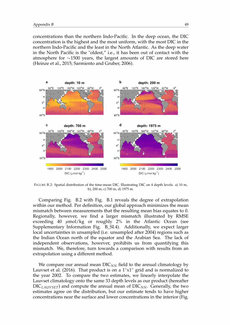
Appendix B 49

concentrations than the northern Indo-Pacific. In the deep ocean, the DICconcentration is the highest and the most uniform, with the most DIC in thenorthern Indo-Pacific and the least in the North Atlantic. As the deep waterin the North Pacific is the "oldest,” i.e., it has been out of contact with theatmosphere for ∼1500 years, the largest amounts of DIC are stored here(Heinze et al., 2015; Sarmiento and Gruber, 2006).

FIGURE B.2: Spatial distribution of the time-mean DIC. Illustrating DIC on 4 depth levels. a) 10 m,b), 200 m, c) 700 m, d) 1975 m.

Comparing Fig. B.2 with Fig. B.1 reveals the degree of extrapolationwithin our method. Per definition, our global approach minimizes the meanmismatch between measurements that the resulting mean bias equates to 0.Regionally, however, we find a larger mismatch illustrated by RMSEexceeding 40 µmol/kg or roughly 2% in the Atlantic Ocean (seeSupplementary Information Fig. B_SI.4). Additionally, we expect largerlocal uncertainties in unsampled (i.e. unsampled after 2004) regions such asthe Indian Ocean north of the equator and the Arabian Sea. The lack ofindependent observations, however, prohibits us from quantifying thismismatch. We, therefore, turn towards a comparison with results from anextrapolation using a different method.

We compare our annual mean DICNN field to the annual climatology byLauvset et al. (2016). That product is on a 1◦x1◦ grid and is normalized tothe year 2002. To compare the two estimates, we linearly interpolate theLauvset climatology onto the same 33 depth levels as our product (hereafterDICLAUVSET) and compute the annual mean of DICNN. Generally, the twoestimates agree on the distribution, but our estimate tends to have higherconcentrations near the surface and lower concentrations in the interior (Fig.

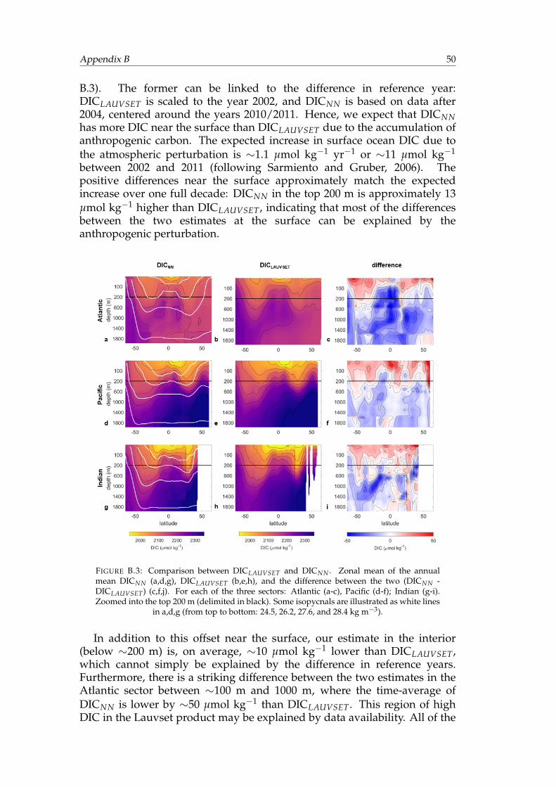
Appendix B 50

B.3). The former can be linked to the difference in reference year:DICLAUVSET is scaled to the year 2002, and DICNN is based on data after2004, centered around the years 2010/2011. Hence, we expect that DICNNhas more DIC near the surface than DICLAUVSET due to the accumulation ofanthropogenic carbon. The expected increase in surface ocean DIC due tothe atmospheric perturbation is ∼1.1 µmol kg−1 yr−1 or ∼11 µmol kg−1

between 2002 and 2011 (following Sarmiento and Gruber, 2006). Thepositive differences near the surface approximately match the expectedincrease over one full decade: DICNN in the top 200 m is approximately 13µmol kg−1 higher than DICLAUVSET, indicating that most of the differencesbetween the two estimates at the surface can be explained by theanthropogenic perturbation.

FIGURE B.3: Comparison between DICLAUVSET and DICNN . Zonal mean of the annualmean DICNN (a,d,g), DICLAUVSET (b,e,h), and the difference between the two (DICNN -DICLAUVSET) (c,f,j). For each of the three sectors: Atlantic (a-c), Pacific (d-f); Indian (g-i).Zoomed into the top 200 m (delimited in black). Some isopycnals are illustrated as white lines

in a,d,g (from top to bottom: 24.5, 26.2, 27.6, and 28.4 kg m−3).

In addition to this offset near the surface, our estimate in the interior(below ∼200 m) is, on average, ∼10 µmol kg−1 lower than DICLAUVSET,which cannot simply be explained by the difference in reference years.Furthermore, there is a striking difference between the two estimates in theAtlantic sector between ∼100 m and 1000 m, where the time-average ofDICNN is lower by ∼50 µmol kg−1 than DICLAUVSET. This region of highDIC in the Lauvset product may be explained by data availability. All of the

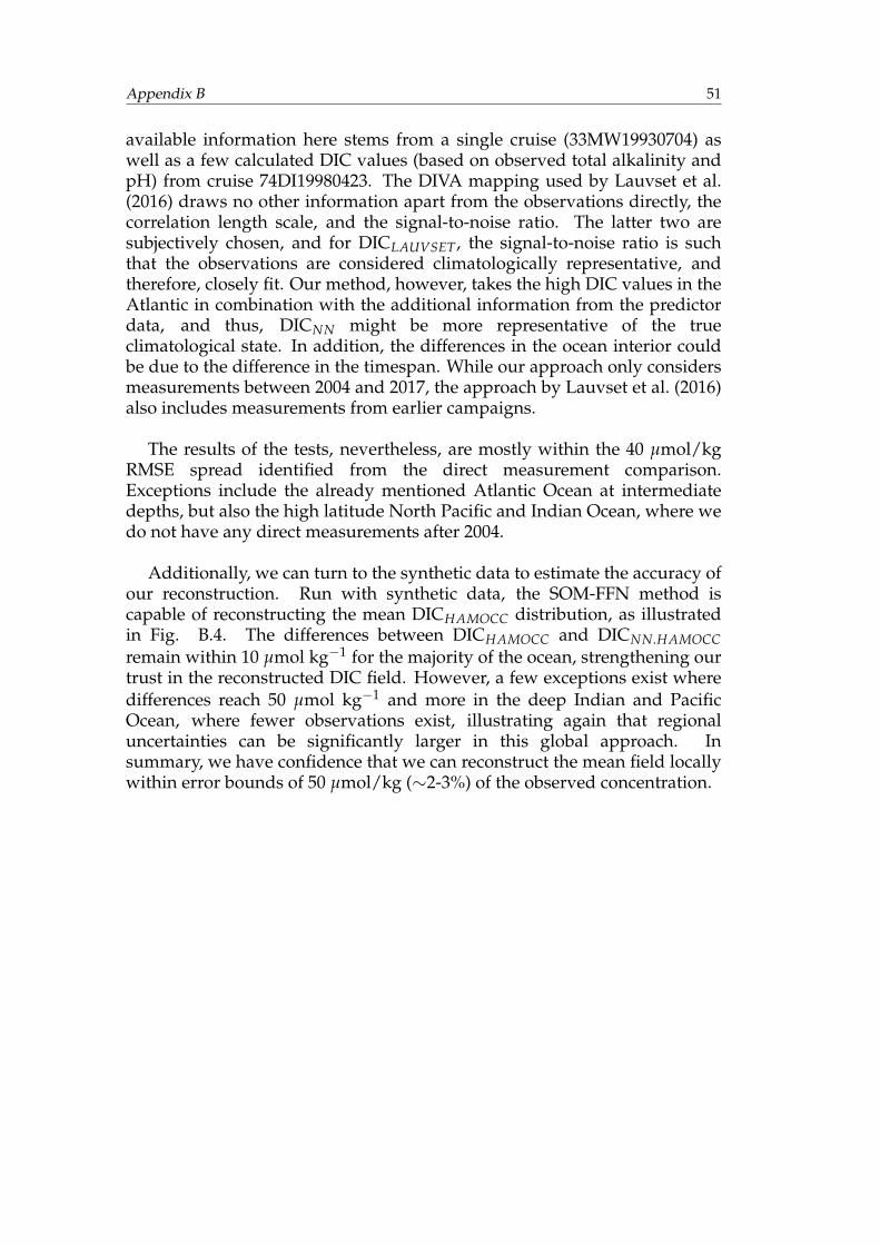
Appendix B 51

available information here stems from a single cruise (33MW19930704) aswell as a few calculated DIC values (based on observed total alkalinity andpH) from cruise 74DI19980423. The DIVA mapping used by Lauvset et al.(2016) draws no other information apart from the observations directly, thecorrelation length scale, and the signal-to-noise ratio. The latter two aresubjectively chosen, and for DICLAUVSET, the signal-to-noise ratio is suchthat the observations are considered climatologically representative, andtherefore, closely fit. Our method, however, takes the high DIC values in theAtlantic in combination with the additional information from the predictordata, and thus, DICNN might be more representative of the trueclimatological state. In addition, the differences in the ocean interior couldbe due to the difference in the timespan. While our approach only considersmeasurements between 2004 and 2017, the approach by Lauvset et al. (2016)also includes measurements from earlier campaigns.

The results of the tests, nevertheless, are mostly within the 40 µmol/kgRMSE spread identified from the direct measurement comparison.Exceptions include the already mentioned Atlantic Ocean at intermediatedepths, but also the high latitude North Pacific and Indian Ocean, where wedo not have any direct measurements after 2004.

Additionally, we can turn to the synthetic data to estimate the accuracy ofour reconstruction. Run with synthetic data, the SOM-FFN method iscapable of reconstructing the mean DICHAMOCC distribution, as illustratedin Fig. B.4. The differences between DICHAMOCC and DICNN.HAMOCCremain within 10 µmol kg−1 for the majority of the ocean, strengthening ourtrust in the reconstructed DIC field. However, a few exceptions exist wheredifferences reach 50 µmol kg−1 and more in the deep Indian and PacificOcean, where fewer observations exist, illustrating again that regionaluncertainties can be significantly larger in this global approach. Insummary, we have confidence that we can reconstruct the mean field locallywithin error bounds of 50 µmol/kg (∼2-3%) of the observed concentration.

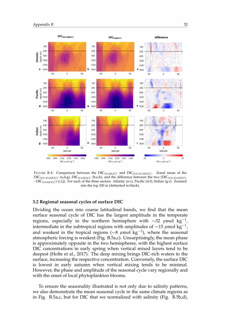
Appendix B 52

FIGURE B.4: Comparison between the DICHAMOCC and DICNN.HAMOCC. Zonal mean of theDICNN.HAMOCC (a,d,g), DICHAMOCC (b,e,h), and the difference between the two (DICNN.HAMOCC- DICHAMOCC) (c,f,j). For each of the three sectors: Atlantic (a-c), Pacific (d-f); Indian (g-i). Zoomed

into the top 200 m (delimited in black).

3.2 Regional seasonal cycles of surface DIC

Dividing the ocean into coarse latitudinal bands, we find that the meansurface seasonal cycle of DIC has the largest amplitude in the temperateregions, especially in the northern hemisphere with ∼32 µmol kg−1,intermediate in the subtropical regions with amplitudes of ∼15 µmol kg−1,and weakest in the tropical regions (∼8 µmol kg−1), where the seasonalatmospheric forcing is weakest (Fig. B.5a,c). Unsurprisingly, the mean phaseis approximately opposite in the two hemispheres, with the highest surfaceDIC concentrations in early spring when vertical mixed layers tend to bedeepest (Holte et al., 2017). The deep mixing brings DIC-rich waters to thesurface, increasing the respective concentration. Conversely, the surface DICis lowest in early autumn when vertical mixing tends to be minimal.However, the phase and amplitude of the seasonal cycle vary regionally andwith the onset of local phytoplankton blooms.

To ensure the seasonality illustrated is not only due to salinity patterns,we also demonstrate the mean seasonal cycle in the same climate regions asin Fig. B.5a,c, but for DIC that we normalized with salinity (Fig. B.5b,d),

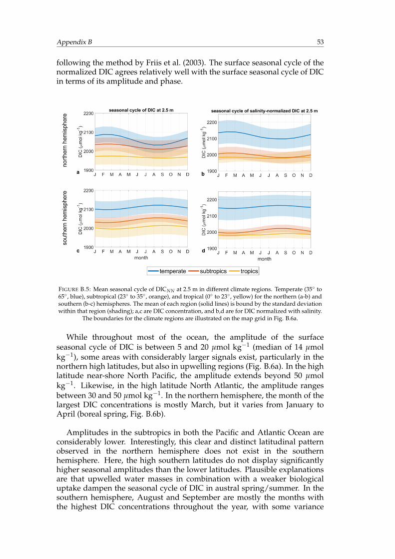
Appendix B 53

following the method by Friis et al. (2003). The surface seasonal cycle of thenormalized DIC agrees relatively well with the surface seasonal cycle of DICin terms of its amplitude and phase.

FIGURE B.5: Mean seasonal cycle of DICNN at 2.5 m in different climate regions. Temperate (35◦ to65◦, blue), subtropical (23◦ to 35◦, orange), and tropical (0◦ to 23◦, yellow) for the northern (a-b) andsouthern (b-c) hemispheres. The mean of each region (solid lines) is bound by the standard deviationwithin that region (shading); a,c are DIC concentration, and b,d are for DIC normalized with salinity.

The boundaries for the climate regions are illustrated on the map grid in Fig. B.6a.

While throughout most of the ocean, the amplitude of the surfaceseasonal cycle of DIC is between 5 and 20 µmol kg−1 (median of 14 µmolkg−1), some areas with considerably larger signals exist, particularly in thenorthern high latitudes, but also in upwelling regions (Fig. B.6a). In the highlatitude near-shore North Pacific, the amplitude extends beyond 50 µmolkg−1. Likewise, in the high latitude North Atlantic, the amplitude rangesbetween 30 and 50 µmol kg−1. In the northern hemisphere, the month of thelargest DIC concentrations is mostly March, but it varies from January toApril (boreal spring, Fig. B.6b).

Amplitudes in the subtropics in both the Pacific and Atlantic Ocean areconsiderably lower. Interestingly, this clear and distinct latitudinal patternobserved in the northern hemisphere does not exist in the southernhemisphere. Here, the high southern latitudes do not display significantlyhigher seasonal amplitudes than the lower latitudes. Plausible explanationsare that upwelled water masses in combination with a weaker biologicaluptake dampen the seasonal cycle of DIC in austral spring/summer. In thesouthern hemisphere, August and September are mostly the months withthe highest DIC concentrations throughout the year, with some variance

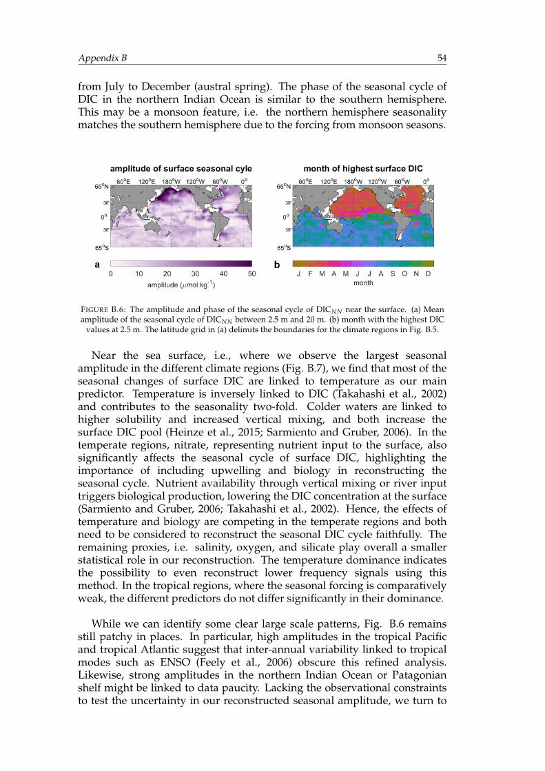
Appendix B 54

from July to December (austral spring). The phase of the seasonal cycle ofDIC in the northern Indian Ocean is similar to the southern hemisphere.This may be a monsoon feature, i.e. the northern hemisphere seasonalitymatches the southern hemisphere due to the forcing from monsoon seasons.

FIGURE B.6: The amplitude and phase of the seasonal cycle of DICNN near the surface. (a) Meanamplitude of the seasonal cycle of DICNN between 2.5 m and 20 m. (b) month with the highest DIC

values at 2.5 m. The latitude grid in (a) delimits the boundaries for the climate regions in Fig. B.5.

Near the sea surface, i.e., where we observe the largest seasonalamplitude in the different climate regions (Fig. B.7), we find that most of theseasonal changes of surface DIC are linked to temperature as our mainpredictor. Temperature is inversely linked to DIC (Takahashi et al., 2002)and contributes to the seasonality two-fold. Colder waters are linked tohigher solubility and increased vertical mixing, and both increase thesurface DIC pool (Heinze et al., 2015; Sarmiento and Gruber, 2006). In thetemperate regions, nitrate, representing nutrient input to the surface, alsosignificantly affects the seasonal cycle of surface DIC, highlighting theimportance of including upwelling and biology in reconstructing theseasonal cycle. Nutrient availability through vertical mixing or river inputtriggers biological production, lowering the DIC concentration at the surface(Sarmiento and Gruber, 2006; Takahashi et al., 2002). Hence, the effects oftemperature and biology are competing in the temperate regions and bothneed to be considered to reconstruct the seasonal DIC cycle faithfully. Theremaining proxies, i.e. salinity, oxygen, and silicate play overall a smallerstatistical role in our reconstruction. The temperature dominance indicatesthe possibility to even reconstruct lower frequency signals using thismethod. In the tropical regions, where the seasonal forcing is comparativelyweak, the different predictors do not differ significantly in their dominance.

While we can identify some clear large scale patterns, Fig. B.6 remainsstill patchy in places. In particular, high amplitudes in the tropical Pacificand tropical Atlantic suggest that inter-annual variability linked to tropicalmodes such as ENSO (Feely et al., 2006) obscure this refined analysis.Likewise, strong amplitudes in the northern Indian Ocean or Patagonianshelf might be linked to data paucity. Lacking the observational constraintsto test the uncertainty in our reconstructed seasonal amplitude, we turn to

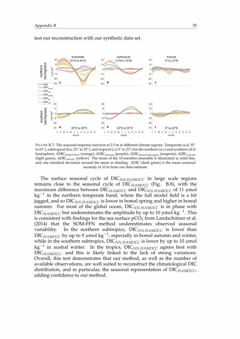
Appendix B 55

test our reconstruction with our synthetic data set.

FIGURE B.7: The seasonal response function at 2.5 m in different climate regions. Temperate (a,d; 35◦

to 65◦), subtropical (b,e; 23◦ to 35◦), and tropical (c,f; 0◦ to 23◦) for the northern (a-c) and southern (d-f)hemisphere, ∆DICtemperature (orange), ∆DICsalinity (purple), ∆DICdissolvedoxygen (magenta), ∆DICsilicate(light green), ∆DICnitrate (yellow). The mean of the 10-member ensemble is illustrated as solid line,and one standard deviation around the mean in shading. ∆DIC (dark green) is the mean seasonal

anomaly at 10 m from our data estimate.

The surface seasonal cycle of DICNN.HAMOCC in large scale regionsremains close to the seasonal cycle of DICHAMOCC (Fig. B.8), with themaximum difference between DICHAMOCC and DICNN.HAMOCC of 11 µmolkg−1 in the northern temperate band, where the full model field is a bitjagged, and so DICNN.HAMOCC is lower in boreal spring and higher in borealsummer. For most of the global ocean, DICNN.HAMOCC is in phase withDICHAMOCC but underestimates the amplitude by up to 10 µmol kg−1. Thisis consistent with findings for the sea surface pCO2 from Landschützer et al.(2014) that the SOM-FFN method underestimates observed seasonalvariability. In the northern subtropics, DICNN.HAMOCC is lower thanDICHAMOCC by up to 9 µmol kg−1, especially in boreal autumn and winter,while in the southern subtropics, DICNN.HAMOCC is lower by up to 10 µmolkg−1 in austral winter. In the tropics, DICNN.HAMOCC agrees best withDICHAMOCC, and this is likely linked to the lack of strong variations.Overall, this test demonstrates that our method, as well as the number ofavailable observations, are well suited to reconstruct the climatological DICdistribution, and in particular, the seasonal representation of DICHAMOCC,adding confidence to our method.

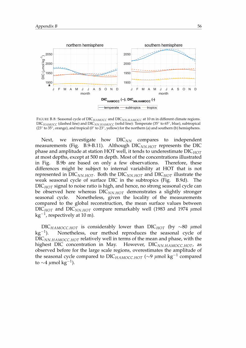
Appendix B 56

FIGURE B.8: Seasonal cycle of DICHAMOCC and DICNN.HAMOCC at 10 m in different climate regions.DICHAMOCC (dashed line) and DICNN.HAMOCC (solid line): Temperate (35◦ to 65◦, blue), subtropical(23◦ to 35◦, orange), and tropical (0◦ to 23◦, yellow) for the northern (a) and southern (b) hemispheres.

Next, we investigate how DICNN compares to independentmeasurements (Fig. B.9-B.11). Although DICNN.HOT represents the DICphase and amplitude at station HOT well, it tends to underestimate DICHOTat most depths, except at 500 m depth. Most of the concentrations illustratedin Fig. B.9b are based on only a few observations. Therefore, thesedifferences might be subject to internal variability at HOT that is notrepresented in DICNN.HOT. Both the DICNN.HOT and DICHOT illustrate theweak seasonal cycle of surface DIC in the subtropics (Fig. B.9d). TheDICHOT signal to noise ratio is high, and hence, no strong seasonal cycle canbe observed here whereas DICNN.HOT demonstrates a slightly strongerseasonal cycle. Nonetheless, given the locality of the measurementscompared to the global reconstruction, the mean surface values betweenDICHOT and DICNN.HOT compare remarkably well (1983 and 1974 µmolkg−1, respectively at 10 m).

DICHAMOCC.HOT is considerably lower than DICHOT (by ∼80 µmolkg−1). Nonetheless, our method reproduces the seasonal cycle ofDICNN.HAMOCC.HOT relatively well in terms of the mean and phase, with thehighest DIC concentration in May. However, DICNN.HAMOCC.HOT, asobserved before for the large scale regions, overestimates the amplitude ofthe seasonal cycle compared to DICHAMOCC.HOT (∼9 µmol kg−1 comparedto ∼4 µmol kg−1).

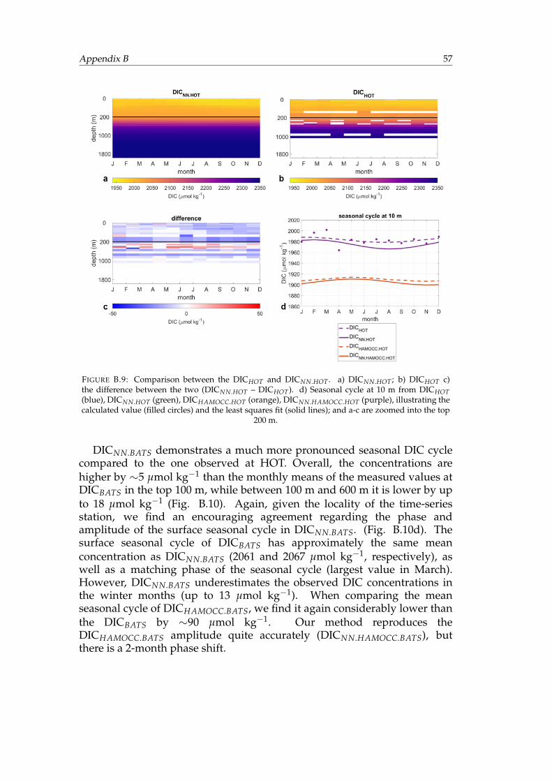
Appendix B 57

FIGURE B.9: Comparison between the DICHOT and DICNN.HOT . a) DICNN.HOT ; b) DICHOT c)the difference between the two (DICNN.HOT – DICHOT). d) Seasonal cycle at 10 m from DICHOT(blue), DICNN.HOT (green), DICHAMOCC.HOT (orange), DICNN.HAMOCC.HOT (purple), illustrating thecalculated value (filled circles) and the least squares fit (solid lines); and a-c are zoomed into the top

200 m.

DICNN.BATS demonstrates a much more pronounced seasonal DIC cyclecompared to the one observed at HOT. Overall, the concentrations arehigher by ∼5 µmol kg−1 than the monthly means of the measured values atDICBATS in the top 100 m, while between 100 m and 600 m it is lower by upto 18 µmol kg−1 (Fig. B.10). Again, given the locality of the time-seriesstation, we find an encouraging agreement regarding the phase andamplitude of the surface seasonal cycle in DICNN.BATS. (Fig. B.10d). Thesurface seasonal cycle of DICBATS has approximately the same meanconcentration as DICNN.BATS (2061 and 2067 µmol kg−1, respectively), aswell as a matching phase of the seasonal cycle (largest value in March).However, DICNN.BATS underestimates the observed DIC concentrations inthe winter months (up to 13 µmol kg−1). When comparing the meanseasonal cycle of DICHAMOCC.BATS, we find it again considerably lower thanthe DICBATS by ∼90 µmol kg−1. Our method reproduces theDICHAMOCC.BATS amplitude quite accurately (DICNN.HAMOCC.BATS), butthere is a 2-month phase shift.

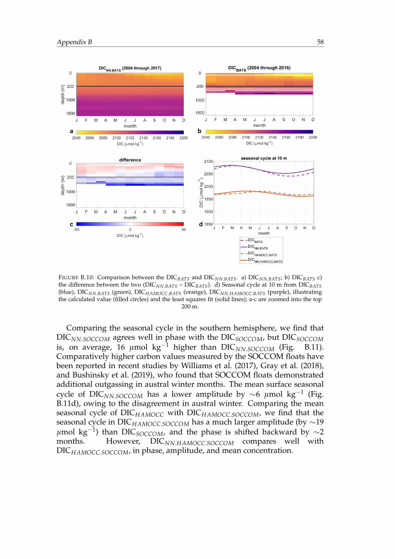
Appendix B 58

FIGURE B.10: Comparison between the DICBATS and DICNN.BATS. a) DICNN.BATS; b) DICBATS c)the difference between the two (DICNN.BATS – DICBATS). d) Seasonal cycle at 10 m from DICBATS(blue), DICNN.BATS (green), DICHAMOCC.BATS (orange), DICNN.HAMOCC.BATS (purple), illustratingthe calculated value (filled circles) and the least squares fit (solid lines); a-c are zoomed into the top

200 m.

Comparing the seasonal cycle in the southern hemisphere, we find thatDICNN.SOCCOM agrees well in phase with the DICSOCCOM, but DICSOCCOMis, on average, 16 µmol kg−1 higher than DICNN.SOCCOM (Fig. B.11).Comparatively higher carbon values measured by the SOCCOM floats havebeen reported in recent studies by Williams et al. (2017), Gray et al. (2018),and Bushinsky et al. (2019), who found that SOCCOM floats demonstratedadditional outgassing in austral winter months. The mean surface seasonalcycle of DICNN.SOCCOM has a lower amplitude by ∼6 µmol kg−1 (Fig.B.11d), owing to the disagreement in austral winter. Comparing the meanseasonal cycle of DICHAMOCC with DICHAMOCC.SOCCOM, we find that theseasonal cycle in DICHAMOCC.SOCCOM has a much larger amplitude (by ∼19µmol kg−1) than DICSOCCOM, and the phase is shifted backward by ∼2months. However, DICNN.HAMOCC.SOCCOM compares well withDICHAMOCC.SOCCOM, in phase, amplitude, and mean concentration.

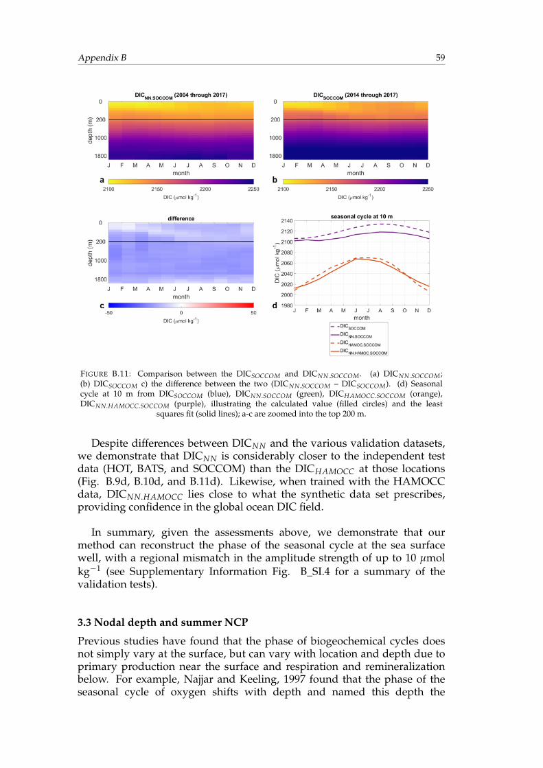
Appendix B 59

FIGURE B.11: Comparison between the DICSOCCOM and DICNN.SOCCOM. (a) DICNN.SOCCOM;(b) DICSOCCOM c) the difference between the two (DICNN.SOCCOM – DICSOCCOM). (d) Seasonalcycle at 10 m from DICSOCCOM (blue), DICNN.SOCCOM (green), DICHAMOCC.SOCCOM (orange),DICNN.HAMOCC.SOCCOM (purple), illustrating the calculated value (filled circles) and the least

squares fit (solid lines); a-c are zoomed into the top 200 m.

Despite differences between DICNN and the various validation datasets,we demonstrate that DICNN is considerably closer to the independent testdata (HOT, BATS, and SOCCOM) than the DICHAMOCC at those locations(Fig. B.9d, B.10d, and B.11d). Likewise, when trained with the HAMOCCdata, DICNN.HAMOCC lies close to what the synthetic data set prescribes,providing confidence in the global ocean DIC field.

In summary, given the assessments above, we demonstrate that ourmethod can reconstruct the phase of the seasonal cycle at the sea surfacewell, with a regional mismatch in the amplitude strength of up to 10 µmolkg−1 (see Supplementary Information Fig. B_SI.4 for a summary of thevalidation tests).

3.3 Nodal depth and summer NCP

Previous studies have found that the phase of biogeochemical cycles doesnot simply vary at the surface, but can vary with location and depth due toprimary production near the surface and respiration and remineralizationbelow. For example, Najjar and Keeling, 1997 found that the phase of theseasonal cycle of oxygen shifts with depth and named this depth the

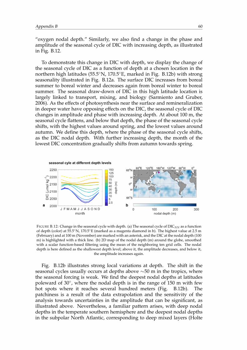
Appendix B 60

“oxygen nodal depth.” Similarly, we also find a change in the phase andamplitude of the seasonal cycle of DIC with increasing depth, as illustratedin Fig. B.12.

To demonstrate this change in DIC with depth, we display the change ofthe seasonal cycle of DIC as a function of depth at a chosen location in thenorthern high latitudes (55.5◦N, 170.5◦E, marked in Fig. B.12b) with strongseasonality illustrated in Fig. B.12a. The surface DIC increases from borealsummer to boreal winter and decreases again from boreal winter to borealsummer. The seasonal draw-down of DIC in this high latitude location islargely linked to transport, mixing, and biology (Sarmiento and Gruber,2006). As the effects of photosynthesis near the surface and remineralizationin deeper water have opposing effects on the DIC, the seasonal cycle of DICchanges in amplitude and phase with increasing depth. At about 100 m, theseasonal cycle flattens, and below that depth, the phase of the seasonal cycleshifts, with the highest values around spring, and the lowest values aroundautumn. We define this depth, where the phase of the seasonal cycle shifts,as the DIC nodal depth. With further increasing depth, the month of thelowest DIC concentration gradually shifts from autumn towards spring.

FIGURE B.12: Change in the seasonal cycle with depth. (a) The seasonal cycle of DICNN as a functionof depth (color) at 55.5◦N, 170.5◦E (marked as a magenta diamond in b). The highest value at 2.5 m(February) and at 100 m (November) are marked with an asterisk, and the DIC at the nodal depth (100m) is highlighted with a thick line. (b) 2D map of the nodal depth (m) around the globe, smoothedwith a scalar function-based filtering using the mean of the neighboring ten grid cells. The nodaldepth is here defined as the shallowest depth level; above it, the amplitude decreases, and below it,

the amplitude increases again.

Fig. B.12b illustrates strong local variations at depth. The shift in theseasonal cycles usually occurs at depths above ∼50 m in the tropics, wherethe seasonal forcing is weak. We find the deepest nodal depths at latitudespoleward of 30◦, where the nodal depth is in the range of 150 m with fewhot spots where it reaches several hundred meters (Fig. B.12b). Thepatchiness is a result of the data extrapolation and the sensitivity of theanalysis towards uncertainties in the amplitude that can be significant, asillustrated above. Nevertheless, a familiar pattern arises, with deep nodaldepths in the temperate southern hemisphere and the deepest nodal depthsin the subpolar North Atlantic, corresponding to deep mixed layers (Holte

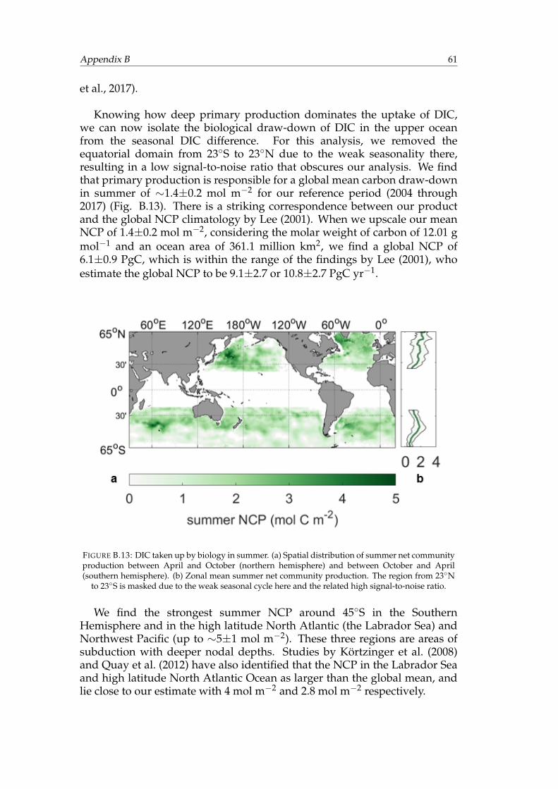
Appendix B 61

et al., 2017).

Knowing how deep primary production dominates the uptake of DIC,we can now isolate the biological draw-down of DIC in the upper oceanfrom the seasonal DIC difference. For this analysis, we removed theequatorial domain from 23◦S to 23◦N due to the weak seasonality there,resulting in a low signal-to-noise ratio that obscures our analysis. We findthat primary production is responsible for a global mean carbon draw-downin summer of ∼1.4±0.2 mol m−2 for our reference period (2004 through2017) (Fig. B.13). There is a striking correspondence between our productand the global NCP climatology by Lee (2001). When we upscale our meanNCP of 1.4±0.2 mol m−2, considering the molar weight of carbon of 12.01 gmol−1 and an ocean area of 361.1 million km2, we find a global NCP of6.1±0.9 PgC, which is within the range of the findings by Lee (2001), whoestimate the global NCP to be 9.1±2.7 or 10.8±2.7 PgC yr−1.

FIGURE B.13: DIC taken up by biology in summer. (a) Spatial distribution of summer net communityproduction between April and October (northern hemisphere) and between October and April(southern hemisphere). (b) Zonal mean summer net community production. The region from 23◦N

to 23◦S is masked due to the weak seasonal cycle here and the related high signal-to-noise ratio.

We find the strongest summer NCP around 45◦S in the SouthernHemisphere and in the high latitude North Atlantic (the Labrador Sea) andNorthwest Pacific (up to ∼5±1 mol m−2). These three regions are areas ofsubduction with deeper nodal depths. Studies by Körtzinger et al. (2008)and Quay et al. (2012) have also identified that the NCP in the Labrador Seaand high latitude North Atlantic Ocean as larger than the global mean, andlie close to our estimate with 4 mol m−2 and 2.8 mol m−2 respectively.

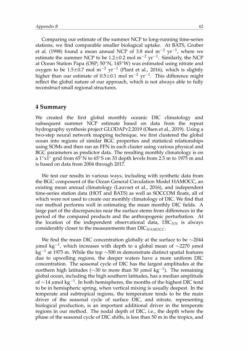
Appendix B 62

Comparing our estimate of the summer NCP to long-running time-seriesstations, we find comparable smaller biological uptake. At BATS, Gruberet al. (1998) found a mean annual NCP of 3.8 mol m−2 yr−1, where weestimate the summer NCP to be 1.2±0.2 mol m−2 yr−1. Similarly, the NCPat Ocean Station Papa (OSP; 50◦N, 145◦W) was estimated using nitrate andoxygen to be 1.5±0.7 mol m−2 yr−1 (Plant et al., 2016), which is slightlyhigher than our estimate of 0.5±0.1 mol m−2 yr−1. This difference mightreflect the global nature of our approach, which is not always able to fullyreconstruct small regional structures.

4 Summary

We created the first global monthly oceanic DIC climatology andsubsequent summer NCP estimate based on data from the repeathydrography synthesis project GLODAPv2.2019 (Olsen et al., 2019). Using atwo-step neural network mapping technique, we first clustered the globalocean into regions of similar BGC properties and statistical relationshipsusing SOMs and then ran an FFN in each cluster using various physical andBGC parameters as predictor data. The resulting monthly climatology is ona 1◦x1◦ grid from 65◦N to 65◦S on 33 depth levels from 2.5 m to 1975 m andis based on data from 2004 through 2017.

We test our results in various ways, including with synthetic data fromthe BGC component of the Ocean General Circulation Model HAMOCC, anexisting mean annual climatology (Lauvset et al., 2016), and independenttime-series station data (HOT and BATS) as well as SOCCOM floats, all ofwhich were not used to create our monthly climatology of DIC. We find thatour method performs well in estimating the mean monthly DIC fields. Alarge part of the discrepancies near the surface stems from differences in theperiod of the compared products and the anthropogenic perturbation. Atthe location of the independent observational data, DICNN is alwaysconsiderably closer to the measurements than DICHAMOCC.

We find the mean DIC concentration globally at the surface to be ∼2044µmol kg−1, which increases with depth to a global mean of ∼2270 µmolkg−1 at 1975 m. While the top ∼500 m demonstrate distinct spatial featuresdue to upwelling regions, the deeper waters have a more uniform DICconcentration. The seasonal cycle of DIC has the largest amplitudes at thenorthern high latitudes (∼30 to more than 50 µmol kg−1). The remainingglobal ocean, including the high southern latitudes, has a median amplitudeof ∼14 µmol kg−1. In both hemispheres, the months of the highest DIC tendto be in hemispheric spring, when vertical mixing is usually deepest. In thetemperate and subtropical regions, the temperature tends to be the maindriver of the seasonal cycle of surface DIC, and nitrate, representingbiological production, is an important additional driver in the temperateregions in our method. The nodal depth of DIC, i.e., the depth where thephase of the seasonal cycle of DIC shifts, is less than 50 m in the tropics, and

Appendix B 63

between 150 and several hundred meters at latitudes poleward of 30◦. Weestimate the carbon draw-down in the upper ocean induced by primaryproduction in hemispheric summer (i.e., the summer NCP) and find thelargest summer NCP in areas of subduction (e.g., around 45◦S, and in thenorthern high latitude Atlantic and West Pacific), in line with previousestimates based on in-situ data. Our estimate suggests a weak butsignificant increase in summer NCP with increasing latitude in the northernhemisphere. Conversely, the maximum summer NCP can be found around45◦S in the southern hemisphere with the least amount of carbon beingtaken up by biology in the high latitude Southern Ocean.

Our monthly climatology provides an advancement to previousclimatologies that have been either limited by their temporal (Lauvset et al.,2016) or spatial domains (Sasse et al., 2013). It provides the baseline toinitialize model set-ups, to study the seasonal cycle of DIC and its futurechanges linked to ocean acidification and to determine the physical andbiogeochemical drivers of the marine carbon cycle. Our DIC-derivedsummer NCP estimate of 1.4±0.2 mol m−2 (∼6.1±0.9 PgC) is in line withprevious observation-based assessments and serves as a complementaryapproach to estimates based on oxygen, which are historically limited intheir temporal and spatial domains (Emerson and Bushinsky, 2014; Emersonet al., 2008; Ostle et al., 2015).

Appendix B 64

Supplementary Information to Appendix B

B_S1 Predictor data

As a neural network reconstructs the available DIC observations based onits relationship to the predictor data, the choice of predictors is essential.Temperature and salinity are known to control the partitioning of DIC intothe chemical species forming the DIC pool: carbonic acid, bicarbonate ions,and carbonate ions (Heinze et al., 2015). In addition to the link betweentemperature and the solubility of CO2 in seawater, both temperature andsalinity also characterize water masses and provide useful additionalinformation about the transport and mixing of DIC (Sarmiento and Gruber,2006). As part of the biological carbon pump, nutrients and oxygen are alsoimportant nominees as predictor data (Heinze et al., 2015), and are availableas monthly climatologies from the World Ocean Atlas 2018 (WOA18;(Garcia et al., 2019)). Therefore, we include temperature, salinity, nitrate,silicate, and dissolved oxygen as predictor data. We do not includephosphate or apparent oxygen utilization (AOU), due to the highcorrelation between nitrate and phosphate, and dissolved oxygen and AOUin most regions. Our results indicate that the network does not gainessential information, while the degrees of freedom substantially increaseby including them. Similarly, we do not include information on the time orlocation as predictor data (for example, latitude, longitude, depth, or monthof the year). See B_S4 for a discussion on this.

We use mapped global data on 1◦x1◦ grids from two different platformsas predictor data. First, we use the optimally interpolated temperature andsalinity fields from the Argo float-based dataset (Argo, 2019; Roemmichet al., 2015). We compute a monthly climatology from 2004 through 2017 ofthese temperature and salinity fields by computing the monthly means. Asthe Argo float-based dataset extends from 2.5 m to 1975 m depth, we usethese depth levels as our minimum and maximum depths, respectively. Wechose 2004 as the starting year as it marks the year where the Argo programprovided global and uniform temperature and salinity data resulting inhigh confidence in the optimally interpolated dataset by Roemmich andGilson (2009).

Second, we use the climatological monthly fields, based on data from1955 through 2017, of dissolved oxygen, silicate, and nitrate from WOA18,which were also mapped using optimal interpolation (Garcia et al., 2019).Here, the dissolved oxygen fields extend until 1500 m, and silicate andnitrate until 500 m. We split the data into three horizontal slabs (2.5–500 m,600–1500 m, 1600–1975 m) and only use the predictors for the respectivedepth slabs where they are available. We then interpolate the predictor dataonto uniform depth levels and normalize the predictor variables to rangebetween 0 and 1. See Table B_SI.1 for a summary of the predictor data andthe respective available depth levels.

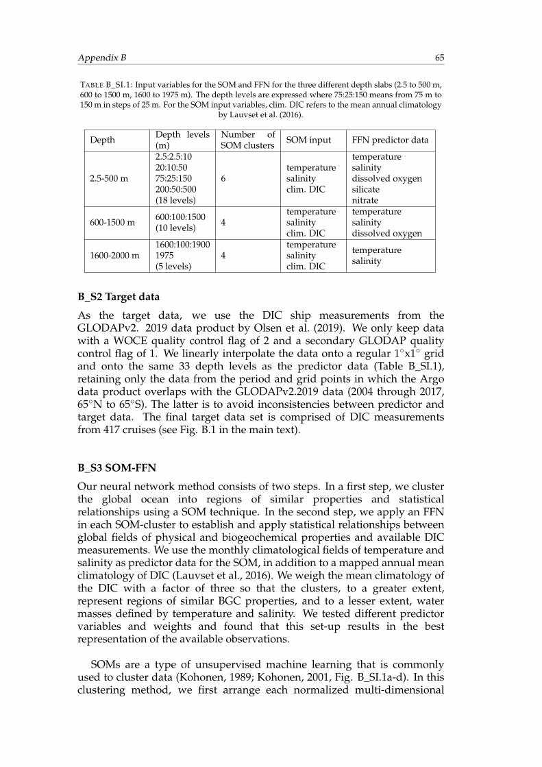
Appendix B 65

TABLE B_SI.1: Input variables for the SOM and FFN for the three different depth slabs (2.5 to 500 m,600 to 1500 m, 1600 to 1975 m). The depth levels are expressed where 75:25:150 means from 75 m to150 m in steps of 25 m. For the SOM input variables, clim. DIC refers to the mean annual climatology

by Lauvset et al. (2016).

Depth Depth levels(m)

Number ofSOM clusters SOM input FFN predictor data

2.5-500 m

2.5:2.5:1020:10:5075:25:150200:50:500(18 levels)

6temperaturesalinityclim. DIC

temperaturesalinitydissolved oxygensilicatenitrate

600-1500 m 600:100:1500(10 levels) 4

temperaturesalinityclim. DIC

temperaturesalinitydissolved oxygen

1600-2000 m1600:100:19001975(5 levels)

4temperaturesalinityclim. DIC

temperaturesalinity

B_S2 Target data

As the target data, we use the DIC ship measurements from theGLODAPv2. 2019 data product by Olsen et al. (2019). We only keep datawith a WOCE quality control flag of 2 and a secondary GLODAP qualitycontrol flag of 1. We linearly interpolate the data onto a regular 1◦x1◦ gridand onto the same 33 depth levels as the predictor data (Table B_SI.1),retaining only the data from the period and grid points in which the Argodata product overlaps with the GLODAPv2.2019 data (2004 through 2017,65◦N to 65◦S). The latter is to avoid inconsistencies between predictor andtarget data. The final target data set is comprised of DIC measurementsfrom 417 cruises (see Fig. B.1 in the main text).

B_S3 SOM-FFN

Our neural network method consists of two steps. In a first step, we clusterthe global ocean into regions of similar properties and statisticalrelationships using a SOM technique. In the second step, we apply an FFNin each SOM-cluster to establish and apply statistical relationships betweenglobal fields of physical and biogeochemical properties and available DICmeasurements. We use the monthly climatological fields of temperature andsalinity as predictor data for the SOM, in addition to a mapped annual meanclimatology of DIC (Lauvset et al., 2016). We weigh the mean climatology ofthe DIC with a factor of three so that the clusters, to a greater extent,represent regions of similar BGC properties, and to a lesser extent, watermasses defined by temperature and salinity. We tested different predictorvariables and weights and found that this set-up results in the bestrepresentation of the available observations.

SOMs are a type of unsupervised machine learning that is commonlyused to cluster data (Kohonen, 1989; Kohonen, 2001, Fig. B_SI.1a-d). In thisclustering method, we first arrange each normalized multi-dimensional

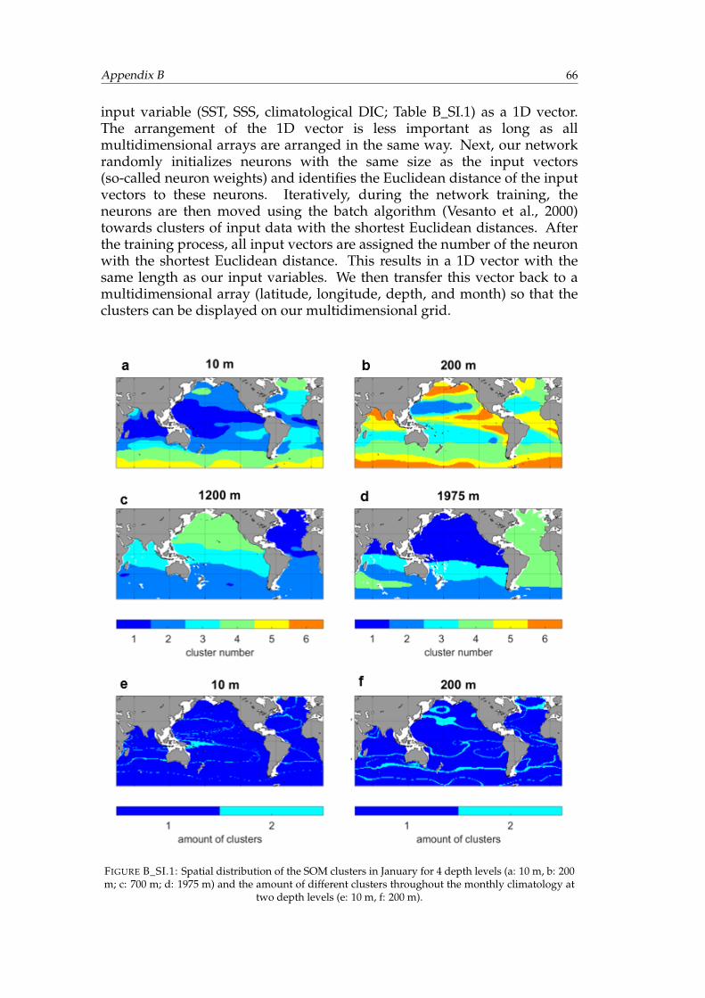
Appendix B 66

input variable (SST, SSS, climatological DIC; Table B_SI.1) as a 1D vector.The arrangement of the 1D vector is less important as long as allmultidimensional arrays are arranged in the same way. Next, our networkrandomly initializes neurons with the same size as the input vectors(so-called neuron weights) and identifies the Euclidean distance of the inputvectors to these neurons. Iteratively, during the network training, theneurons are then moved using the batch algorithm (Vesanto et al., 2000)towards clusters of input data with the shortest Euclidean distances. Afterthe training process, all input vectors are assigned the number of the neuronwith the shortest Euclidean distance. This results in a 1D vector with thesame length as our input variables. We then transfer this vector back to amultidimensional array (latitude, longitude, depth, and month) so that theclusters can be displayed on our multidimensional grid.

FIGURE B_SI.1: Spatial distribution of the SOM clusters in January for 4 depth levels (a: 10 m, b: 200m; c: 700 m; d: 1975 m) and the amount of different clusters throughout the monthly climatology at

two depth levels (e: 10 m, f: 200 m).

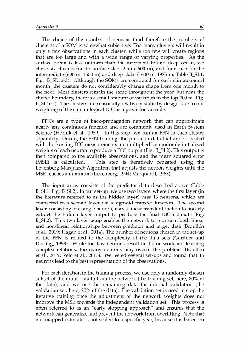
Appendix B 67

The choice of the number of neurons (and therefore the numbers ofclusters) of a SOM is somewhat subjective. Too many clusters will result inonly a few observations in each cluster, while too few will create regionsthat are too large and with a wide range of varying properties. As thesurface ocean is less uniform than the intermediate and deep ocean, wechose six clusters for the surface slab (2.5 m–500 m), and four each for theintermediate (600 m–1500 m) and deep slabs (1600 m–1975 m; Table B_SI.1;Fig. B_SI.1a-d). Although the SOMs are computed for each climatologicalmonth, the clusters do not considerably change shape from one month tothe next. Most clusters remain the same throughout the year, but near thecluster boundary, there is a small amount of variation in the top 200 m (Fig.B_SI.1e-f). The clusters are seasonally relatively static by design due to ourweighting of the climatological DIC as a predictor variable.

FFNs are a type of back-propagation network that can approximatenearly any continuous function and are commonly used in Earth SystemScience (Hornik et al., 1989). In this step, we run an FFN in each clusterseparately. During the FFN training, the predictor data that are co-locatedwith the existing DIC measurements are multiplied by randomly initializedweights of each neuron to produce a DIC output (Fig. B_SI.2). This output isthen compared to the available observations, and the mean squared error(MSE) is calculated. This step is iteratively repeated using theLevenberg-Marquardt Algorithm that adjusts the neuron weights until theMSE reaches a minimum (Levenberg, 1944; Marquardt, 1963).

The input array consists of the predictor data described above (TableB_SI.1, Fig. B_SI.2). In our set-up, we use two layers, where the first layer (inthe literature referred to as the hidden layer) uses 16 neurons, which areconnected to a second layer via a sigmoid transfer function. The secondlayer, consisting of a single neuron, uses a linear transfer function to linearlyextract the hidden layer output to produce the final DIC estimate (Fig.B_SI.2). This two-layer setup enables the network to represent both linearand non-linear relationships between predictor and target data (Broullónet al., 2019; Hagan et al., 2014). The number of neurons chosen in the set-upof the FFN is related to the complexity of the data sets (Gardner andDorling, 1998). While too few neurons result in the network not learningcomplex relations, too many neurons may overfit the problem (Broullónet al., 2019; Velo et al., 2013). We tested several set-ups and found that 16neurons lead to the best representation of the observations.

For each iteration in the training process, we use only a randomly chosensubset of the input data to train the network (the training set; here, 80% ofthe data), and we use the remaining data for internal validation (thevalidation set; here, 20% of the data). The validation set is used to stop theiterative training once the adjustment of the network weights does notimprove the MSE towards the independent validation set. This process isoften referred to as an “early stopping approach” and ensures that thenetwork can generalize and prevent the network from overfitting. Note thatour mapped estimate is not scaled to a specific year, because it is based on

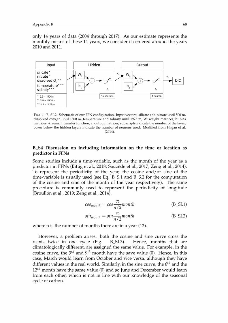
Appendix B 68

only 14 years of data (2004 through 2017). As our estimate represents themonthly means of these 14 years, we consider it centered around the years2010 and 2011.

FIGURE B_SI.2: Schematic of our FFN configuration. Input vectors: silicate and nitrate until 500 m,dissolved oxygen until 1500 m, temperature and salinity until 1975 m; W: weight matrices; b: biasmatrices, +: sum; f: transfer function; a: output matrices; subscripts indicate the number of the layer;boxes below the hidden layers indicate the number of neurons used. Modified from Hagan et al.

(2014).

B_S4 Discussion on including information on the time or location aspredictor in FFNs

Some studies include a time-variable, such as the month of the year as apredictor in FFNs (Bittig et al., 2018; Sauzède et al., 2017; Zeng et al., 2014).To represent the periodicity of the year, the cosine and/or sine of thetime-variable is usually used (see Eq. B_S.1 and B_S.2 for the computationof the cosine and sine of the month of the year respectively). The sameprocedure is commonly used to represent the periodicity of longitude(Broullón et al., 2019; Zeng et al., 2014).

cosmonth = cosπ

n/2month (B_SI.1)

sinmonth = sinπ

n/2month (B_SI.2)

where n is the number of months there are in a year (12).

However, a problem arises: both the cosine and sine curve cross thex-axis twice in one cycle (Fig. B_SI.3). Hence, months that areclimatologically different, are assigned the same value. For example, in thecosine curve, the 3rd and 9th month have the save value (0). Hence, in thiscase, March would learn from October and vice versa, although they havedifferent values in the real world. Similarly, in the sine curve, the 6th and the12th month have the same value (0) and so June and December would learnfrom each other, which is not in line with our knowledge of the seasonalcycle of carbon.

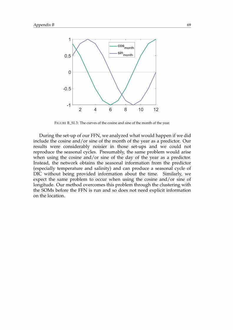
Appendix B 69

FIGURE B_SI.3: The curves of the cosine and sine of the month of the year.

During the set-up of our FFN, we analyzed what would happen if we didinclude the cosine and/or sine of the month of the year as a predictor. Ourresults were considerably noisier in those set-ups and we could notreproduce the seasonal cycles. Presumably, the same problem would arisewhen using the cosine and/or sine of the day of the year as a predictor.Instead, the network obtains the seasonal information from the predictor(especially temperature and salinity) and can produce a seasonal cycle ofDIC without being provided information about the time. Similarly, weexpect the same problem to occur when using the cosine and/or sine oflongitude. Our method overcomes this problem through the clustering withthe SOMs before the FFN is run and so does not need explicit informationon the location.

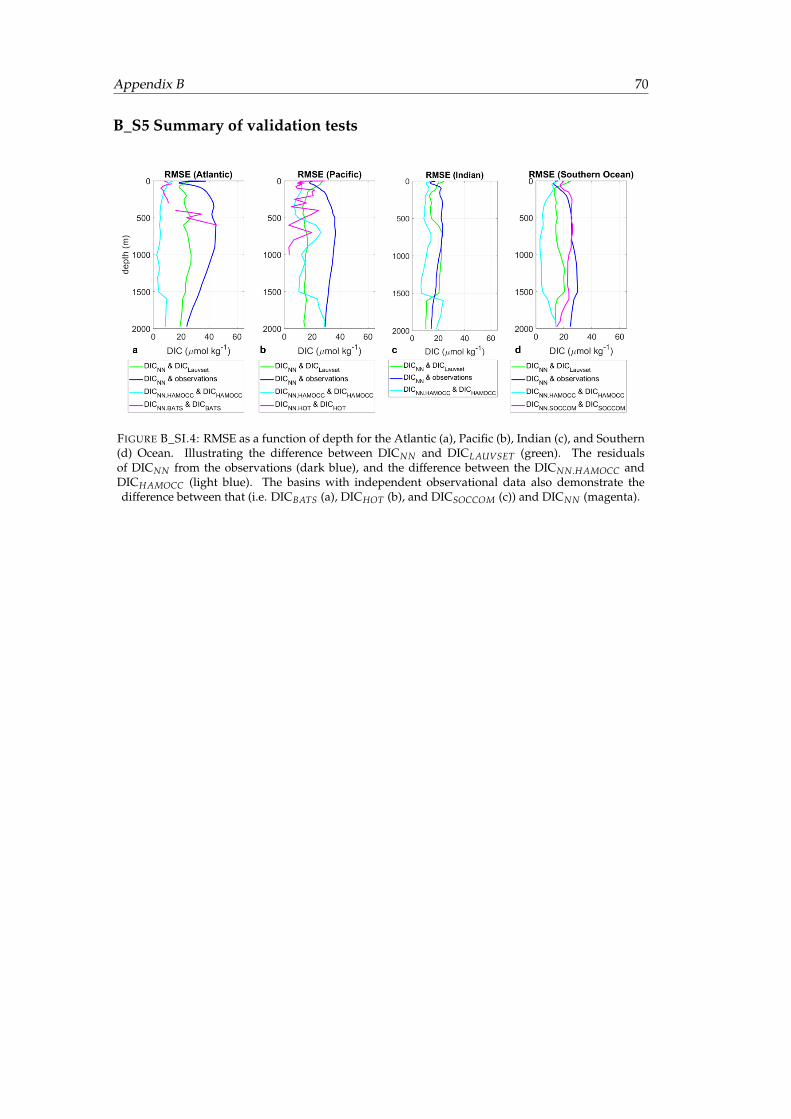
Appendix B 70

B_S5 Summary of validation tests

FIGURE B_SI.4: RMSE as a function of depth for the Atlantic (a), Pacific (b), Indian (c), and Southern(d) Ocean. Illustrating the difference between DICNN and DICLAUVSET (green). The residualsof DICNN from the observations (dark blue), and the difference between the DICNN.HAMOCC andDICHAMOCC (light blue). The basins with independent observational data also demonstrate thedifference between that (i.e. DICBATS (a), DICHOT (b), and DICSOCCOM (c)) and DICNN (magenta).

71

C Temporary Reduction in Southern Ocean sub-surfaceDissolved Inorganic Carbon

Keppler, Lydia1,2 & Peter Landschützer1

1 Max-Planck-Institute for Meteorology (MPI-M), Hamburg, Germany.2 International Max Planck Research School on Earth System Modelling(IMPRS-ESM), Hamburg, Germany.

Paper status at the time of the submission of this thesis:In preparation, to be submitted to Geophysical Research Letters

Data availability:The data product created during this study is freely available to the public(will be submitted to NCEI OCADS after publication of this paper).

Supplementary Information accompanies this paper at the end of thisAppendix.

Contributions: L.K. and P.L. designed the research; L.K. performed the research;L.K. wrote the draft manuscript; P.L. contributed to the discussion of the results andthe manuscript at all stages.

Appendix C 72

Abstract

The Southern Ocean carbon sink is highly variable. However, it is unclearhow this variability is reflected in the dissolved inorganic carbon (DIC) pool,and the drivers behind this variability are still debated. Here, we repeathydrography measurements of DIC from the GLODAPv2.2019 database incombination with a 2-step mapping approach to obtain monthly globalfields of interior DIC from 2004 through 2017 to investigate the interannualsignal until 500 m depth in the Southern Ocean south of 35◦S. At the seasurface, the strongest signal is the anthropogenically-forced DIC trend withlittle variations resulting from reduced sub-surface DIC transport. Belowthe surface, we discover a more pronounced DIC reduction up to ∼20 µmolkg−1 from 2004 through 2009, followed by a strong recovery until 2012. Thisreduction is most prominent south of the Polar Front and extends to 500 m.These sub-surface variations are largely in line with proposed variations inthe meridional overturning circulation during this period.

1 Introduction

Approximately half of the oceanic uptake of anthropogenic carbon dioxidefrom the atmosphere occurs in the Southern Ocean south of 35◦S, althoughthis region covers approximately 1/3 of the global oceans (Landschützeret al., 2015). Different, often opposing processes are at play here, affectingthe carbon flux, and the transport and storage of carbon at depth. Close tothe Antarctic coast, sea-water is cooled, which allows for oceanic carbonuptake due to enhanced solubility, and the down-welling of thesecarbon-enriched surface waters stores it at depth. Near the AntarcticCircumpolar Current (ACC), northward Ekman transport inducesupwelling of carbon-rich waters and thereby outgassing of carbon. North ofthe ACC, Subantarctic Mode Waters that are transported northwards coolthe warmer subtropical waters, leading to oceanic uptake of carbon, whichis then subducted and transported northward. However, these processesdisplay a large degree of variability on time scales from interannual todecadal (DeVries et al., 2017; Downes et al., 2009; Freeman et al., 2016; Halland Visbeck, 2002; Schlosser et al., 2018).

The Southern Ocean carbon uptake at the air-sea interface was found tohave weakened in the 1990s, despite the continued increase in atmosphericCO2 (Le Quéré et al., 2007). This finding led to concern that the SouthernOcean carbon sink could have saturated. However, nearly a decade later,Landschützer et al. (2015) found that this globally important carbon sinkhad regained its strength between 2002 and 2011 and was back at thestrength as would be expected due to the increase in atmospheric CO2.Recently, the trend has reversed again, and from 2012 through 2016 theSouthern Ocean carbon sink weakened again (Keppler and Landschützer,2019).

Appendix C 73

The mechanisms explaining these decadal changes in the Southern Oceancarbon sink are not yet fully resolved and relate to circulation and biology.(Gruber et al., 2019a; Keppler and Landschützer, 2019; Landschützer et al.,2015) proposed that these changes are linked to regional variability in thelocal weather pattern, causing different hot spots of air-sea CO2 exchange.DeVries et al. (2017) linked a weakening of the Meridional OverturningCirculation (MOC) in the 2000s to a strengthening of the Southern Oceancarbon uptake due to less upward transport and outgassing of naturalcarbon stored at depth. Similarly, Panassa et al. (2018) proposed linksbetween the Southern Ocean carbon uptake variability and changes in thesummer mixed layer depth in that region, as a deeper mixed layer enhancesvertical mixing and thus, biological uptake of carbon. In line with thatfinding, Gregor et al. (2018) found that the biological draw-down of carbonis the main driver of the seasonal variability in the Southern Ocean carbonflux. As changes in the MOC and the biological uptake of carbon arereflected in the dissolved inorganic carbon (DIC) pool, we choose toinvestigate the recent development of the interior DIC in the SouthernOcean.

Most of the oceanic carbon that is taken up from the atmosphere is storedat depth as DIC, while a smaller amount is drawn down throughphotosynthesizing organisms consuming carbon (Heinze et al., 2015;Keppler et al., in review). Previous studies on the changes in the stored DIConly focused on the anthropogenic part and did so at decadal time-scales(Gruber et al., 2019b; Khatiwala et al., 2009; Sabine et al., 2004) as their focuswas the anthropogenic increase rather than interannual to decadalvariations of the DIC pool. Specifically, Gruber et al. (2019b) found that halfof the global anthropogenic DIC occupies the upper 400 m, and theSouthern Ocean has the second-deepest vertical extent of anthropogeniccarbon in the world, only exceeded in the Deep Water Formation region ofthe North Atlantic. As the interannual to decadal variability of the carbonuptake at the surface is quite substantial (Keppler and Landschützer, 2019;Landschützer et al., 2015; Le Quéré et al., 2007), one would expect to seesome of this variability in the interior DIC. The temporal-mean distributionof DIC in the water column, as well as the seasonal cycle of DIC, has beenestimated by previous global-scale studies (Keppler et al., in review;Lauvset et al., 2016). However, the interannual to decadal variations in theinterior Southern Ocean contemporary DIC (natural + anthropogenic) is yetto be investigated.

The processes of upwelling and subduction, and the associated carbonfluxes and storage, are not zonally uniform and many processes in theSouthern Ocean occur in ’hot spots’ (Rintoul, 2018; Sallée et al., 2012). Toinvestigate the variability in the DIC pool at a regional scale, a mapped dataestimate of DIC in the Southern Ocean, based on available but sparseshipboard measurements, is necessary. Recent progress in the collection andsynthesis of available observations through the Global Ocean Data AnalysisProject for Carbon (GLODAP, Key et al. (2015) and Olsen et al. (2019)) hasled to the compilation of ship-measurements of oceanic carbon in the

Appendix C 74

interior ocean from the surface until over 7000 m depth. The data consists ofover 1.1 million direct measurements from bottled sea-water samples acrossthe world since the 1970s. However, despite an increase in shipmeasurements through the repeat hydrography surveys (Talley et al., 2016),DIC measurements in the Southern Ocean remain sparse.

Here, we combine data from GLODAPv2.2019 with a two-stepneural-network-based mapping technique to reconstruct mapped monthlyinterior DIC fields from 2004 through 2017 for the global ocean. Using ournew data estimate, we present the variability of DIC in the top 500 m of theSouthern Ocean and link the observed variability both to processes thatdrive this variability and to processes that are driven by it.

2 Data and Methods

This section briefly discusses the novel set-up of our method and the dataused. A more detailed discussion on the method can be found in Keppleret al. (in review). In the first step, we cluster the global ocean into regionsthat have similar biogeochemical properties using self-organizing maps(SOMs), and in a second step, we run a Feed-Forward-Network (FFN) ineach of the clusters. The FFN first approximates the statistical relationshipbetween predictor data and target data within each SOM-cluster and thenapplies this relationship to infer the oceanic DIC concentration. We usemonthly gridded DIC fields from 2004 through 2017 from GLODAPv2.2019(Key et al., 2015; Olsen et al., 2019) as target data. Following Keppler et al.(in review), temperature, salinity, dissolved oxygen, silicate, and nitrate areall useful predictors of the seasonal cycle of DIC as these predictors not onlydrive the partitioning of DIC through the physical and biological carbonpump but also are statistically tied to DIC by defining different watermasses; hence, we use the same predictors for our updated set-up.

Compared to the monthly climatology by Keppler et al. (in review), weextend our data product to a monthly temporal resolution from 2004through 2017 and chose a vertical extent of 500 m. Below this depth, fewerobservations exist, and we expect little variability in the DIC pool oninterannual to decadal timescales (Gruber et al., 2019b). In the SOM-step,we use six clusters, following Keppler et al. (in review). In the FFN-step, weuse the objectively interpolated interannual fields of temperature andsalinity based on Argo float measurements (Argo, 2019; Roemmich andGilson, 2009) as predictors. This data product is on a 1◦x1◦ grid and reachesfrom 65◦N to 65◦S, and from 2.5 m to 1975 m. In addition, we use theobjectively interpolated monthly climatologies of dissolved oxygen, silicate,and nitrate from the World Ocean Atlas 2018 (Garcia et al., 2019). Althoughthese variables are only available at seasonal resolution, these predictors aidin the reconstruction of the distribution of interior DIC. To reconstruct theexpected trend from the increase in atmospheric CO2, we further use themonthly fields of the oceanic surface pCO2 (Landschützer et al., 2014) andthe globally averaged annual mean concentration of atmospheric CO2 at the

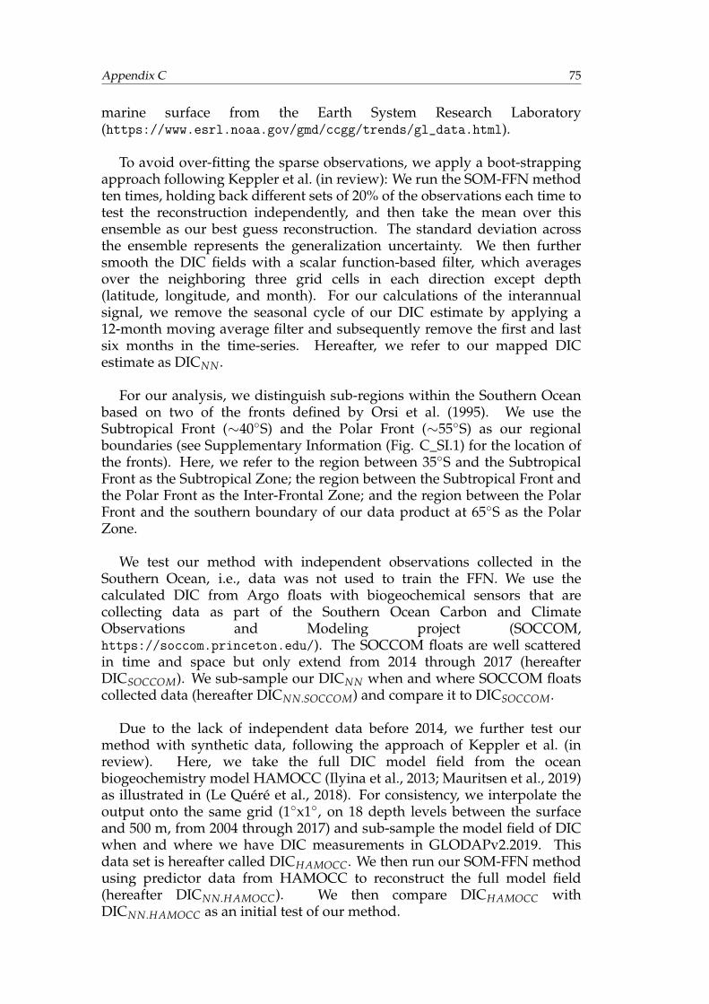
Appendix C 75

marine surface from the Earth System Research Laboratory(https://www.esrl.noaa.gov/gmd/ccgg/trends/gl_data.html).

To avoid over-fitting the sparse observations, we apply a boot-strappingapproach following Keppler et al. (in review): We run the SOM-FFN methodten times, holding back different sets of 20% of the observations each time totest the reconstruction independently, and then take the mean over thisensemble as our best guess reconstruction. The standard deviation acrossthe ensemble represents the generalization uncertainty. We then furthersmooth the DIC fields with a scalar function-based filter, which averagesover the neighboring three grid cells in each direction except depth(latitude, longitude, and month). For our calculations of the interannualsignal, we remove the seasonal cycle of our DIC estimate by applying a12-month moving average filter and subsequently remove the first and lastsix months in the time-series. Hereafter, we refer to our mapped DICestimate as DICNN.

For our analysis, we distinguish sub-regions within the Southern Oceanbased on two of the fronts defined by Orsi et al. (1995). We use theSubtropical Front (∼40◦S) and the Polar Front (∼55◦S) as our regionalboundaries (see Supplementary Information (Fig. C_SI.1) for the location ofthe fronts). Here, we refer to the region between 35◦S and the SubtropicalFront as the Subtropical Zone; the region between the Subtropical Front andthe Polar Front as the Inter-Frontal Zone; and the region between the PolarFront and the southern boundary of our data product at 65◦S as the PolarZone.

We test our method with independent observations collected in theSouthern Ocean, i.e., data was not used to train the FFN. We use thecalculated DIC from Argo floats with biogeochemical sensors that arecollecting data as part of the Southern Ocean Carbon and ClimateObservations and Modeling project (SOCCOM,https://soccom.princeton.edu/). The SOCCOM floats are well scatteredin time and space but only extend from 2014 through 2017 (hereafterDICSOCCOM). We sub-sample our DICNN when and where SOCCOM floatscollected data (hereafter DICNN.SOCCOM) and compare it to DICSOCCOM.

Due to the lack of independent data before 2014, we further test ourmethod with synthetic data, following the approach of Keppler et al. (inreview). Here, we take the full DIC model field from the oceanbiogeochemistry model HAMOCC (Ilyina et al., 2013; Mauritsen et al., 2019)as illustrated in (Le Quéré et al., 2018). For consistency, we interpolate theoutput onto the same grid (1◦x1◦, on 18 depth levels between the surfaceand 500 m, from 2004 through 2017) and sub-sample the model field of DICwhen and where we have DIC measurements in GLODAPv2.2019. Thisdata set is hereafter called DICHAMOCC. We then run our SOM-FFN methodusing predictor data from HAMOCC to reconstruct the full model field(hereafter DICNN.HAMOCC). We then compare DICHAMOCC withDICNN.HAMOCC as an initial test of our method.

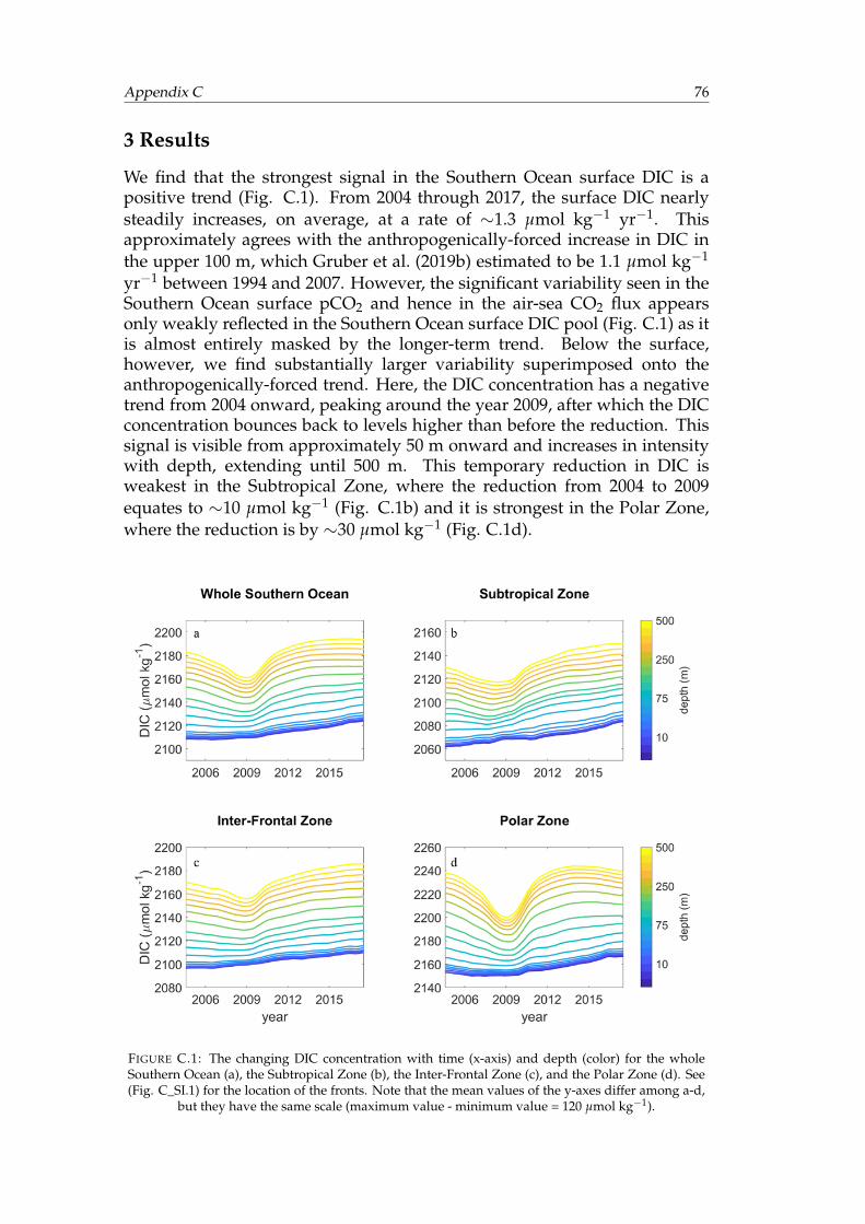
Appendix C 76

3 Results

We find that the strongest signal in the Southern Ocean surface DIC is apositive trend (Fig. C.1). From 2004 through 2017, the surface DIC nearlysteadily increases, on average, at a rate of ∼1.3 µmol kg−1 yr−1. Thisapproximately agrees with the anthropogenically-forced increase in DIC inthe upper 100 m, which Gruber et al. (2019b) estimated to be 1.1 µmol kg−1

yr−1 between 1994 and 2007. However, the significant variability seen in theSouthern Ocean surface pCO2 and hence in the air-sea CO2 flux appearsonly weakly reflected in the Southern Ocean surface DIC pool (Fig. C.1) as itis almost entirely masked by the longer-term trend. Below the surface,however, we find substantially larger variability superimposed onto theanthropogenically-forced trend. Here, the DIC concentration has a negativetrend from 2004 onward, peaking around the year 2009, after which the DICconcentration bounces back to levels higher than before the reduction. Thissignal is visible from approximately 50 m onward and increases in intensitywith depth, extending until 500 m. This temporary reduction in DIC isweakest in the Subtropical Zone, where the reduction from 2004 to 2009equates to ∼10 µmol kg−1 (Fig. C.1b) and it is strongest in the Polar Zone,where the reduction is by ∼30 µmol kg−1 (Fig. C.1d).

FIGURE C.1: The changing DIC concentration with time (x-axis) and depth (color) for the wholeSouthern Ocean (a), the Subtropical Zone (b), the Inter-Frontal Zone (c), and the Polar Zone (d). See(Fig. C_SI.1) for the location of the fronts. Note that the mean values of the y-axes differ among a-d,

but they have the same scale (maximum value - minimum value = 120 µmol kg−1).

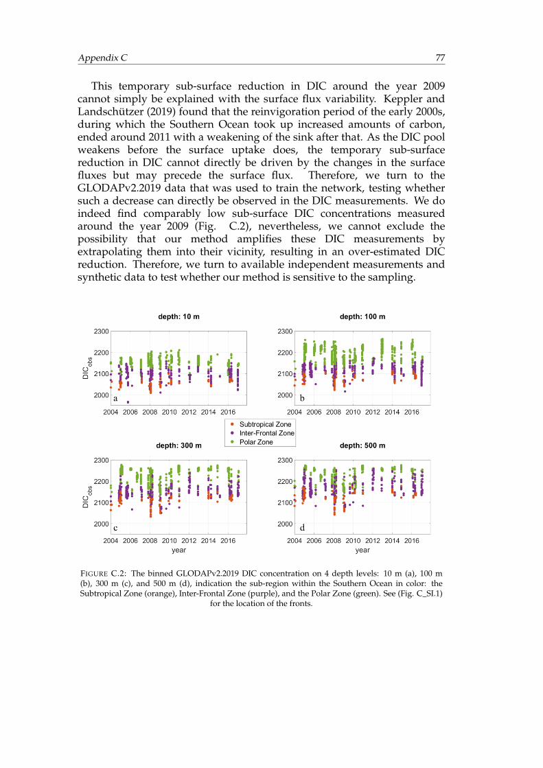
Appendix C 77

This temporary sub-surface reduction in DIC around the year 2009cannot simply be explained with the surface flux variability. Keppler andLandschützer (2019) found that the reinvigoration period of the early 2000s,during which the Southern Ocean took up increased amounts of carbon,ended around 2011 with a weakening of the sink after that. As the DIC poolweakens before the surface uptake does, the temporary sub-surfacereduction in DIC cannot directly be driven by the changes in the surfacefluxes but may precede the surface flux. Therefore, we turn to theGLODAPv2.2019 data that was used to train the network, testing whethersuch a decrease can directly be observed in the DIC measurements. We doindeed find comparably low sub-surface DIC concentrations measuredaround the year 2009 (Fig. C.2), nevertheless, we cannot exclude thepossibility that our method amplifies these DIC measurements byextrapolating them into their vicinity, resulting in an over-estimated DICreduction. Therefore, we turn to available independent measurements andsynthetic data to test whether our method is sensitive to the sampling.

FIGURE C.2: The binned GLODAPv2.2019 DIC concentration on 4 depth levels: 10 m (a), 100 m(b), 300 m (c), and 500 m (d), indication the sub-region within the Southern Ocean in color: theSubtropical Zone (orange), Inter-Frontal Zone (purple), and the Polar Zone (green). See (Fig. C_SI.1)

for the location of the fronts.

Appendix C 78

We test whether our method can reconstruct the calculated DIC fromSOCCOM floats, which was not used to train the network, and thereforeprovide an independent dataset. While the SOCCOM floats started profilingin 2014, they cannot resolve the 2009 reduction, however, they provide abenchmark test, whether our method is capable of reconstructing theobserved DIC concentration and variability in the later years of our study.From 2014 onward, the trend and interannual variability in DICNN.SOCCOMcompares remarkably well to DICSOCCOM (Fig. C.3a-d), given theindependent nature of these measurements. There is, however, an offset inthe mean concentration of approximately 10 µmol kg−1, withDICNN.SOCCOM being generally lower than DICSOCCOM. This offset may, inpart, also be explained by the fact that DIC is not directly measured by thefloats and is calculated from directly observed quantities. The root meansquared error (RMSE) between DICNN.SOCCOM and DICSOCCOM equates to24 µmol kg−1 largely owing to the mean offset. Nevertheless, given theindependent nature of the float data and the fact that we compare calculatedDIC from floats to an extrapolation of sparse ship data, we find anencouraging agreement between them.

To test whether the signal results from data sparsity and a largesignal-to-noise ratio in the measurements, we use synthetic data from ahindcast simulation of the ocean biogeochemistry model HAMOCC, forcedwith real climate (DICHAMOCC). We subsample DICHAMOCC at the time andlocation of the GLODAPv2.2019 ship tracks and then reconstruct the modelfield using our 2-step neural network method and predictor data from theHAMOCC model (DICNN.HAMOCC). Both the mean DIC concentration andthe interannual variability of DICNN.HAMOCC in the Southern Oceancompares well with DICHAMOCC (Fig. C.3e). Unlike the real-worldreconstruction, the model field does not display significantly strongervariability at depth compared to the surface. Overall, besides a few smalldiscrepancies, the RMSE between DICNN.HAMOCC and DICHAMOCC is only 8µmol kg−1, increasing the confidence in our reconstruction. This RMSE isconsiderably smaller compared to the SOCCOM comparison, which can beexplained by the larger amount of noise in measurements compared to thesmoother model field.

We can further use the HAMOCC model output to test whether the meanoffset from the SOCCOM float comparison (Fig. C.3a-d) is an artifact of theshipboard sampling. Therefore, as an additional test, we sub-sampleDICHAMOCC at the time and location of SOCCOM float measurements(hereafter DICHAMOCC.SOCCOM). The SOM-FFN reconstructionDICNN.SOCCOM lies considerably closer to DIC SOCCOM thanDICHAMOCC.SOCCOM. However, DICNN.HAMOCC.SOCCOM reconstructsDICHAMOCC.SOCCOM very well with a small RMSE of 9 µmol kg−1 (Fig.C.3)a-d) that is in the range of the overall RMSE from the full modelreconstruction above.

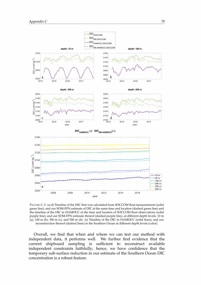
Appendix C 79

FIGURE C.3: (a-d) Timeline of the DIC that was calculated from SOCCOM float measurements (solidgreen line), and our SOM-FFN estimate of DIC at the same time and location (dashed green line) andthe timeline of the DIC in HAMOCC at the time and location of SOCCOM float observations (solidpurple line), and our SOM-FFN estimate thereof (dashed purple line), at different depth levels: 10 m(a), 100 m (b), 300 m (c), and 500 m (d). (e) Timeline of the DIC in HAMOCC (solid lines), and our

reconstruction thereof (dashed lines) in the Southern Ocean at different depth levels (color).

Overall, we find that when and where we can test our method withindependent data, it performs well. We further find evidence that thecurrent shipboard sampling is sufficient to reconstruct availableindependent constraints faithfully; hence, we have confidence that thetemporary sub-surface reduction in our estimate of the Southern Ocean DICconcentration is a robust feature.

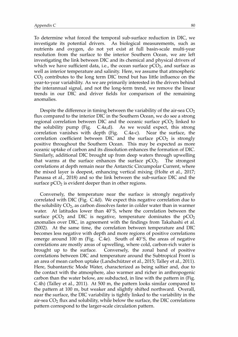
Appendix C 80

To determine what forced the temporal sub-surface reduction in DIC, weinvestigate its potential drivers. As biological measurements, such asnutrients and oxygen, do not yet exist at full basin-scale multi-yearresolution from the surface to the interior Southern Ocean, we are leftinvestigating the link between DIC and its chemical and physical drivers ofwhich we have sufficient data, i.e., the ocean surface pCO2, and surface aswell as interior temperature and salinity. Here, we assume that atmosphericCO2 contributes to the long term DIC trend but has little influence on theyear-to-year variability. As we are primarily interested in the drivers behindthe interannual signal, and not the long-term trend, we remove the lineartrends in our DIC and driver fields for comparison of the remaininganomalies.

Despite the difference in timing between the variability of the air-sea CO2flux compared to the interior DIC in the Southern Ocean, we do see a strongregional correlation between DIC and the oceanic surface pCO2 linked tothe solubility pump (Fig. C.4a,d). As we would expect, this strongcorrelation vanishes with depth (Fig. C.4a-c). Near the surface, thecorrelation coefficient between DIC and the surface pCO2 is stronglypositive throughout the Southern Ocean. This may be expected as moreoceanic uptake of carbon and its dissolution enhances the formation of DIC.Similarly, additional DIC brought up from deep waters through upwellingthat warms at the surface enhances the surface pCO2. The strongestcorrelations at depth remain near the Antarctic Circumpolar Current, wherethe mixed layer is deepest, enhancing vertical mixing (Holte et al., 2017;Panassa et al., 2018) and so the link between the sub-surface DIC and thesurface pCO2 is evident deeper than in other regions.

Conversely, the temperature near the surface is strongly negativelycorrelated with DIC (Fig. C.4d). We expect this negative correlation due tothe solubility CO2, as carbon dissolves faster in colder water than in warmerwater. At latitudes lower than 40◦S, where the correlation between thesurface pCO2 and DIC is negative, temperature dominates the pCO2anomalies over DIC, in agreement with the findings from Takahashi et al.(2002). At the same time, the correlation between temperature and DICbecomes less negative with depth and more regions of positive correlationsemerge around 100 m (Fig. C.4e). South of 40◦S, the areas of negativecorrelations are mostly areas of upwelling, where cold, carbon-rich water isbrought up to the surface. Conversely, the zonal band of positivecorrelations between DIC and temperature around the Subtropical Front isan area of mean carbon uptake (Landschützer et al., 2015; Talley et al., 2011).Here, Subantarctic Mode Water, characterized as being saltier and, due tothe contact with the atmosphere, also warmer and richer in anthropogeniccarbon than the water below, are subducted, in line with the pattern in (Fig.C.4h) (Talley et al., 2011). At 500 m, the pattern looks similar compared tothe pattern at 100 m, but weaker and slightly shifted northward. Overall,near the surface, the DIC variability is tightly linked to the variability in theair-sea CO2 flux and solubility, while below the surface, the DIC correlationspattern correspond to the larger-scale circulation pattern.

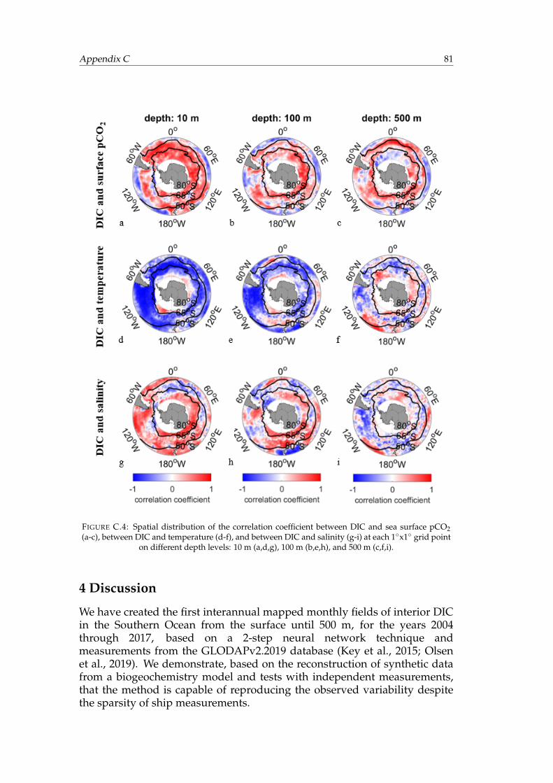
Appendix C 81

FIGURE C.4: Spatial distribution of the correlation coefficient between DIC and sea surface pCO2(a-c), between DIC and temperature (d-f), and between DIC and salinity (g-i) at each 1◦x1◦ grid point

on different depth levels: 10 m (a,d,g), 100 m (b,e,h), and 500 m (c,f,i).

4 Discussion

We have created the first interannual mapped monthly fields of interior DICin the Southern Ocean from the surface until 500 m, for the years 2004through 2017, based on a 2-step neural network technique andmeasurements from the GLODAPv2.2019 database (Key et al., 2015; Olsenet al., 2019). We demonstrate, based on the reconstruction of synthetic datafrom a biogeochemistry model and tests with independent measurements,that the method is capable of reproducing the observed variability despitethe sparsity of ship measurements.

Appendix C 82

Our results reveal that variations, as seen in the surface uptake of carbon(Keppler et al., in review; Landschützer et al., 2015; Le Quéré et al., 2007),are visible in the water column, albeit near the surface, these variations aresmall in comparison to the trend driven by the increase in anthropogenicCO2. We further find a substantial decadal signal in the DIC below thesurface, with a minimum in 2009, followed by a quick recovery after that.This signal extends to at least 500 m and is also seen in the directGLODAPv2.2019 observations. This signal is strongest in the Polar Zone,i.e., near the Antarctic coast, which is an area of upwelling and outgassing.

The observed sub-surface variability and the driver correlations line upwith recent findings by DeVries et al. (2017), i.e. that the observed variationsin the global carbon flux are related to changes in the MOC. The authorsused a global inverse model to quantify the MOC and found that astrengthened MOC in the 1990s enhanced the outgassing of carbon, while inthe 2000s, a weaker MOC led to less outgassing of natural carbon and thus,larger net oceanic uptake of carbon. Although that study does not extend tothe 2010s, it supports our finding until 2009. The weaker MOC leads to lesssub-surface DIC as suppressed overturning results in a weaker upwardtransport of natural carbon from the deep Subantarctic and Antarctic watermasses. Likewise, the sub-surface correlations between DIC, temperatureand salinity, their negative link in upwelling as well as their positive link insubduction regions further supports the connection to the MOC variability.Furthermore, Panassa et al. (2018) found that the summer mixed layer depthdeepened by 2 m yr−1 between 2002 and 2011 near the Subtropical Front, i.e.a region of outgassing in which we find sub-surface DIC positivelycorrelates with surface pCO2 and negatively with temperature. Thus, theobserved changes in sub-surface DIC can again be linked to physicalsub-surface processes.

Both the variability in the Southern Ocean MOC and the changes inmixed-layer depth have been linked to variability in the Southern AnnularMode (SAM), the dominant mode of climate variability in this region(DeVries et al., 2017; Marshall, 2003; Panassa et al., 2018). During positivephases in the SAM, the westerly winds strengthen and shift poleward (Halland Visbeck, 2002), thus enhancing and shifting the MOC. Between 2004and 2009, the SAM index polarity was low in comparison to the late 1990sand 2010s (Supplementary Information (Fig. C_SI.2. This may indicatefurther that a slower MOC caused the sub-surface reduction in DIC. Thus,our study provides further observation-based evidence to the study ofDeVries et al. (2017) that the link between the strong variability in theSouthern Ocean air-sea CO2 flux (Keppler and Landschützer, 2019;Landschützer et al., 2015; Le Quéré et al., 2007) is linked to the MOC-drivenchanges in sub-surface DIC.

The link to the MOC and SAM, might, at first sight, appear contradictoryto the findings by Keppler and Landschützer (2019), as these authorspropose that trends in the SAM have a zero net effect on the overallcontemporary air-sea CO2 flux trends, whereas regional wind variability

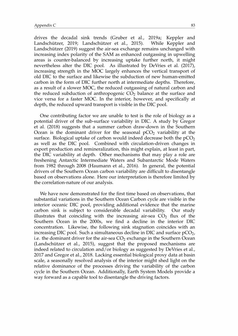
Appendix C 83

drives the decadal sink trends (Gruber et al., 2019a; Keppler andLandschützer, 2019; Landschützer et al., 2015). While Keppler andLandschützer (2019) suggest the air-sea exchange remains unchanged withincreasing index polarity of the SAM as enhanced outgassing in upwellingareas is counter-balanced by increasing uptake further north, it mightnevertheless alter the DIC pool. As illustrated by DeVries et al. (2017),increasing strength in the MOC largely enhances the vertical transport ofold DIC to the surface and likewise the subduction of new human-emittedcarbon in the form of DIC further north at intermediate depths. Therefore,as a result of a slower MOC, the reduced outgassing of natural carbon andthe reduced subduction of anthropogenic CO2 balance at the surface andvice versa for a faster MOC. In the interior, however, and specifically atdepth, the reduced upward transport is visible in the DIC pool.

One contributing factor we are unable to test is the role of biology as apotential driver of the sub-surface variability in DIC. A study by Gregoret al. (2018) suggests that a summer carbon draw-down in the SouthernOcean is the dominant driver for the seasonal pCO2 variability at thesurface. Biological uptake of carbon would indeed decrease both the pCO2as well as the DIC pool. Combined with circulation-driven changes inexport production and remineralization, this might explain, at least in part,the DIC variability at depth. Other mechanisms that may play a role arefreshening Antarctic Intermediate Waters and Subantarctic Mode Watersfrom 1982 through 2008 (Haumann et al., 2016). In general, the potentialdrivers of the Southern Ocean carbon variability are difficult to disentanglebased on observations alone. Here our interpretation is therefore limited bythe correlation-nature of our analysis.

We have now demonstrated for the first time based on observations, thatsubstantial variations in the Southern Ocean Carbon cycle are visible in theinterior oceanic DIC pool, providing additional evidence that the marinecarbon sink is subject to considerable decadal variability. Our studyillustrates that coinciding with the increasing air-sea CO2 flux of theSouthern Ocean in the 2000s, we find a decline in the interior DICconcentration. Likewise, the following sink stagnation coincides with anincreasing DIC pool. Such a simultaneous decline in DIC and surface pCO2,i.e. the dominant driver for the air-sea CO2 exchange in the Southern Ocean(Landschützer et al., 2015), suggest that the proposed mechanisms areindeed related to circulation and/or biology as suggested by DeVries et al.,2017 and Gregor et al., 2018. Lacking essential biological proxy data at basinscale, a seasonally resolved analysis of the interior might shed light on therelative dominance of the processes driving the variability of the carboncycle in the Southern Ocean. Additionally, Earth System Models provide away forward as a capable tool to disentangle the driving factors.

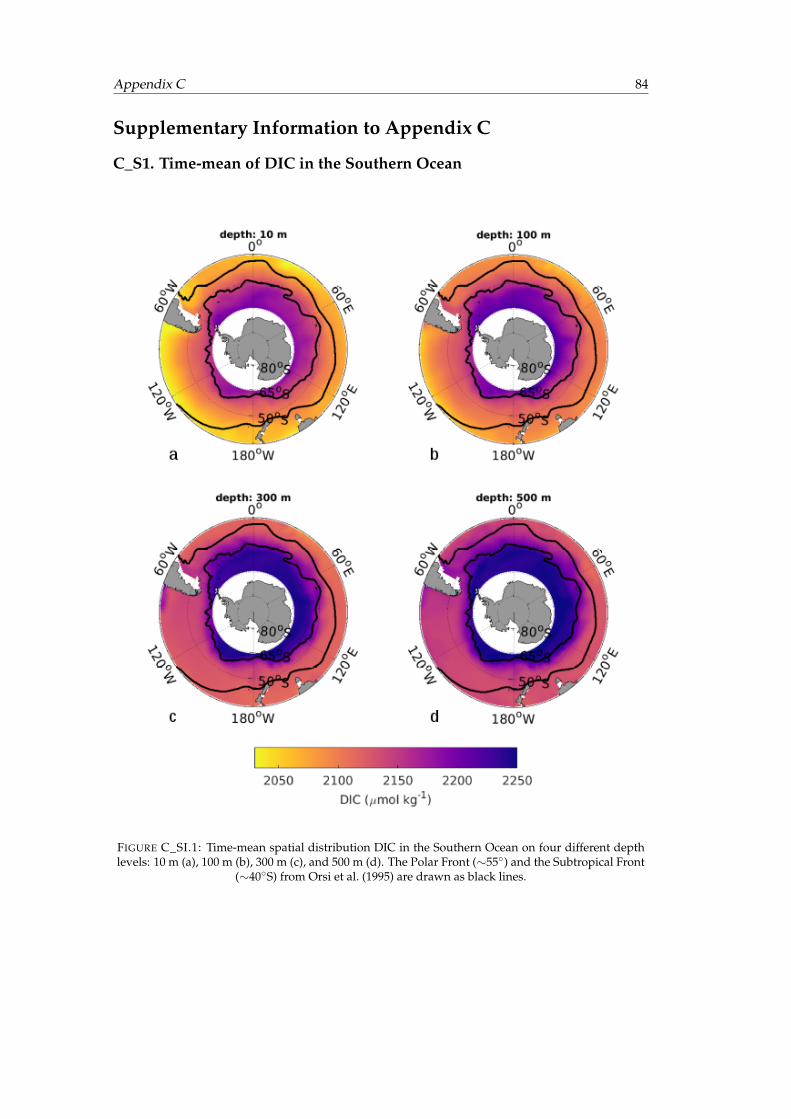
Appendix C 84

Supplementary Information to Appendix C

C_S1. Time-mean of DIC in the Southern Ocean

FIGURE C_SI.1: Time-mean spatial distribution DIC in the Southern Ocean on four different depthlevels: 10 m (a), 100 m (b), 300 m (c), and 500 m (d). The Polar Front (∼55◦) and the Subtropical Front

(∼40◦S) from Orsi et al. (1995) are drawn as black lines.

Appendix C 85

C_S2. Timeline of the recent SAM

FIGURE C_SI.2: Timeline of the recent SAM index from Marshall (2003) (black line), smoothed witha 12-month running-mean (red/blue).

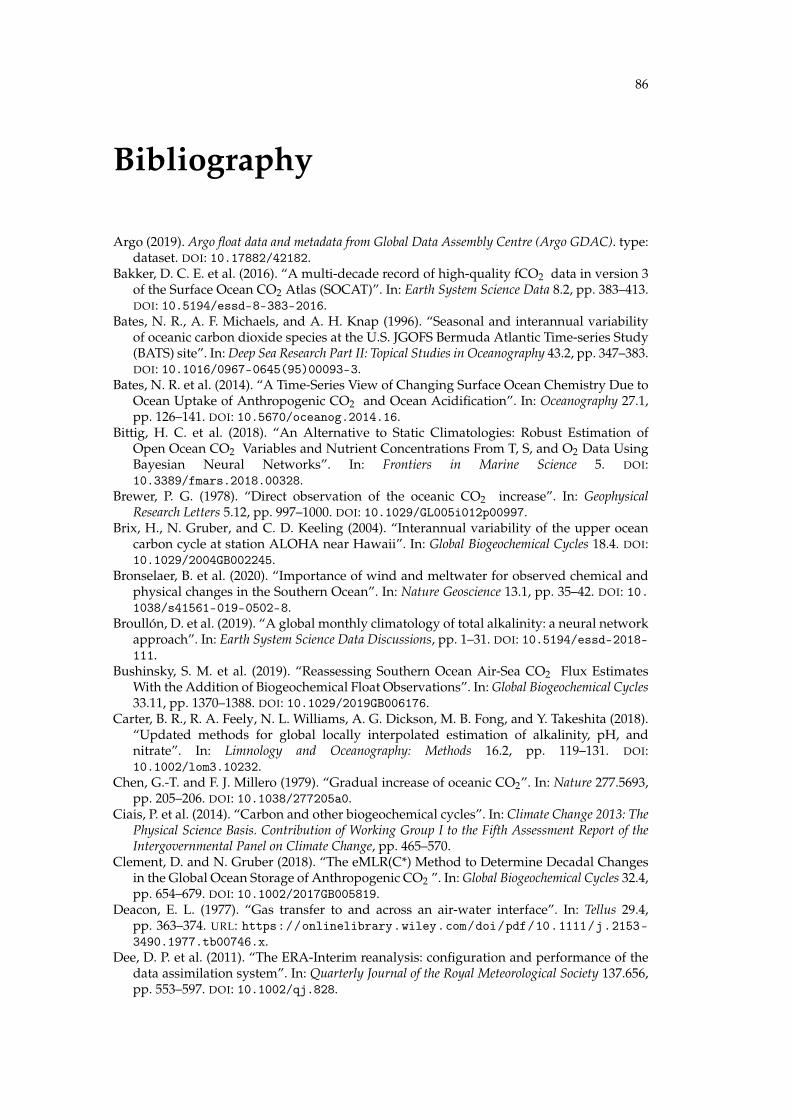
86

Bibliography

Argo (2019). Argo float data and metadata from Global Data Assembly Centre (Argo GDAC). type:dataset. DOI: 10.17882/42182.

Bakker, D. C. E. et al. (2016). “A multi-decade record of high-quality fCO2 data in version 3of the Surface Ocean CO2 Atlas (SOCAT)”. In: Earth System Science Data 8.2, pp. 383–413.DOI: 10.5194/essd-8-383-2016.

Bates, N. R., A. F. Michaels, and A. H. Knap (1996). “Seasonal and interannual variabilityof oceanic carbon dioxide species at the U.S. JGOFS Bermuda Atlantic Time-series Study(BATS) site”. In: Deep Sea Research Part II: Topical Studies in Oceanography 43.2, pp. 347–383.DOI: 10.1016/0967-0645(95)00093-3.

Bates, N. R. et al. (2014). “A Time-Series View of Changing Surface Ocean Chemistry Due toOcean Uptake of Anthropogenic CO2 and Ocean Acidification”. In: Oceanography 27.1,pp. 126–141. DOI: 10.5670/oceanog.2014.16.

Bittig, H. C. et al. (2018). “An Alternative to Static Climatologies: Robust Estimation ofOpen Ocean CO2 Variables and Nutrient Concentrations From T, S, and O2 Data UsingBayesian Neural Networks”. In: Frontiers in Marine Science 5. DOI:10.3389/fmars.2018.00328.

Brewer, P. G. (1978). “Direct observation of the oceanic CO2 increase”. In: GeophysicalResearch Letters 5.12, pp. 997–1000. DOI: 10.1029/GL005i012p00997.

Brix, H., N. Gruber, and C. D. Keeling (2004). “Interannual variability of the upper oceancarbon cycle at station ALOHA near Hawaii”. In: Global Biogeochemical Cycles 18.4. DOI:10.1029/2004GB002245.

Bronselaer, B. et al. (2020). “Importance of wind and meltwater for observed chemical andphysical changes in the Southern Ocean”. In: Nature Geoscience 13.1, pp. 35–42. DOI: 10.1038/s41561-019-0502-8.

Broullón, D. et al. (2019). “A global monthly climatology of total alkalinity: a neural networkapproach”. In: Earth System Science Data Discussions, pp. 1–31. DOI: 10.5194/essd-2018-111.

Bushinsky, S. M. et al. (2019). “Reassessing Southern Ocean Air-Sea CO2 Flux EstimatesWith the Addition of Biogeochemical Float Observations”. In: Global Biogeochemical Cycles33.11, pp. 1370–1388. DOI: 10.1029/2019GB006176.

Carter, B. R., R. A. Feely, N. L. Williams, A. G. Dickson, M. B. Fong, and Y. Takeshita (2018).“Updated methods for global locally interpolated estimation of alkalinity, pH, andnitrate”. In: Limnology and Oceanography: Methods 16.2, pp. 119–131. DOI:10.1002/lom3.10232.

Chen, G.-T. and F. J. Millero (1979). “Gradual increase of oceanic CO2”. In: Nature 277.5693,pp. 205–206. DOI: 10.1038/277205a0.

Ciais, P. et al. (2014). “Carbon and other biogeochemical cycles”. In: Climate Change 2013: ThePhysical Science Basis. Contribution of Working Group I to the Fifth Assessment Report of theIntergovernmental Panel on Climate Change, pp. 465–570.

Clement, D. and N. Gruber (2018). “The eMLR(C*) Method to Determine Decadal Changesin the Global Ocean Storage of Anthropogenic CO2 ”. In: Global Biogeochemical Cycles 32.4,pp. 654–679. DOI: 10.1002/2017GB005819.

Deacon, E. L. (1977). “Gas transfer to and across an air-water interface”. In: Tellus 29.4,pp. 363–374. URL: https://onlinelibrary.wiley.com/doi/pdf/10.1111/j.2153-3490.1977.tb00746.x.

Dee, D. P. et al. (2011). “The ERA-Interim reanalysis: configuration and performance of thedata assimilation system”. In: Quarterly Journal of the Royal Meteorological Society 137.656,pp. 553–597. DOI: 10.1002/qj.828.

Bibliography 87

DeVries, T. (2014). “The oceanic anthropogenic CO2 sink: Storage, air-sea fluxes, and trans-ports over the industrial era”. In: Global Biogeochemical Cycles 28.7, pp. 631–647. DOI: 10.1002/2013GB004739.

DeVries, T., M. Holzer, and F. Primeau (2017). “Recent increase in oceanic carbon uptakedriven by weaker upper-ocean overturning”. In: Nature 542.7640, pp. 215–218. DOI: 10.1038/nature21068.

Dibike, Y. B. and P. Coulibaly (2006). “Temporal neural networks for downscaling climatevariability and extremes”. In: Neural Networks. Earth Sciences and EnvironmentalApplications of Computational Intelligence 19.2, pp. 135–144. DOI:10.1016/j.neunet.2006.01.003.

Dickson, A. G., C. L. Sabine, J. R. Christian, C. P. Bargeron, and N. P. M. S. Organization, eds.(2007). Guide to best practices for ocean CO2 measurements. PICES special publication no. 3.OCLC: ocn420872251. Sidney, BC: North Pacific Marine Science Organization. 1 p. ISBN:978-1-897176-07-8.

Doney, S. C., V. J. Fabry, R. A. Feely, and J. A. Kleypas (2009). “Ocean Acidification: TheOther CO2 Problem”. In: Annual Review of Marine Science 1.1. Publisher: Annual Reviews,pp. 169–192. DOI: 10.1146/annurev.marine.010908.163834.

Dore, J. E., R. Lukas, D. W. Sadler, M. J. Church, and D. M. Karl (2009). “Physical andbiogeochemical modulation of ocean acidification in the central North Pacific”. In:Proceedings of the National Academy of Sciences of the United States of America 106.30,pp. 12235–12240. DOI: 10.1073/pnas.0906044106.

Dore, J. E., R. Lukas, D. W. Sadler, and D. M. Karl (2003). “Climate-driven changes to theatmospheric CO2 sink in the subtropical North Pacific Ocean”. In: Nature 424.6950,pp. 754–757. DOI: 10.1038/nature01885.

Downes, S. M., A. S. Budnick, J. L. Sarmiento, and R. Farneti (2011). “Impacts of wind stresson the Antarctic Circumpolar Current fronts and associated subduction”. In: GeophysicalResearch Letters 38.11. DOI: 10.1029/2011GL047668.

Downes, S. M., N. L. Bindoff, and S. R. Rintoul (2009). “Impacts of Climate Change on theSubduction of Mode and Intermediate Water Masses in the Southern Ocean”. In: Journalof Climate 22.12, pp. 3289–3302. DOI: 10.1175/2008JCLI2653.1.

Emerson, S. and S. Bushinsky (2014). “Oxygen Concentrations and Biological Fluxes in theOpen Ocean”. In: Oceanography 27.1, pp. 168–171. DOI: 10.5670/oceanog.2014.20.

Emerson, S., C. Stump, and D. Nicholson (2008). “Net biological oxygen production in theocean: Remote in situ measurements of O2 and N2 in surface waters”. In: GlobalBiogeochemical Cycles 22.3. DOI: 10.1029/2007GB003095.

Feely, R. A. et al. (2006). “Decadal variability of the air-sea CO2 fluxes in the equatorialPacific Ocean”. In: Journal of Geophysical Research: Oceans 111 (C8). DOI:10.1029/2005JC003129.

Fogt, R. L., J. M. Jones, and J. Renwick (2012). “Seasonal Zonal Asymmetries in the SouthernAnnular Mode and Their Impact on Regional Temperature Anomalies”. In: Journal ofClimate 25.18, pp. 6253–6270. DOI: 10.1175/JCLI-D-11-00474.1.

Freeman, N. M., N. S. Lovenduski, and P. R. Gent (2016). “Temporal variability in theAntarctic Polar Front (2002-2014)”. In: Journal of Geophysical Research-Oceans 121.10,pp. 7263–7276. DOI: 10.1002/2016JC012145.

Friedlingstein, P. et al. (2019). “Global Carbon Budget 2019”. In: Earth System Science Data11.4, pp. 1783–1838. DOI: 10.5194/essd-11-1783-2019.

Friis, K., A. Körtzinger, and D. W. R. Wallace (2003). “The salinity normalization of marineinorganic carbon chemistry data”. In: Geophysical Research Letters 30.2. DOI: 10.1029/2002GL015898.

Frölicher, T. L., J. L. Sarmiento, D. J. Paynter, J. P. Dunne, J. P. Krasting, and M. Winton (2015).“Dominance of the Southern Ocean in Anthropogenic Carbon and Heat Uptake in CMIP5Models”. In: Journal of Climate 28.2, pp. 862–886. DOI: 10.1175/JCLI-D-14-00117.1.

Garcia, H. et al. (2019). World Ocean Atlas 2018: Product Documentation. Ed. by A. Mishonov.Gardner, M. W. and S. R. Dorling (1998). “Artificial neural networks (the multilayer

perceptron)—a review of applications in the atmospheric sciences”. In: AtmosphericEnvironment 32, pp. 2627–2636. DOI: 10.1016/S1352-2310(97)00447-0.

Bibliography 88

Gevrey, M., I. Dimopoulos, and S. Lek (2003). “Review and comparison of methods to studythe contribution of variables in artificial neural network models”. In: Ecological Modelling.Modelling the structure of aquatic communities: concepts, methods, and problems. 160.3,pp. 249–264. DOI: 10.1016/S0304-3800(02)00257-0.

Gray, A. R. et al. (2018). “Autonomous biogeochemical floats detect significant carbondioxide outgassing in the high-latitude Southern Ocean”. In: Geophysical Research Letters0 (ja). DOI: 10.1029/2018GL078013.

Gregor, L., S. Kok, and P. M. S. Monteiro (2018). “Interannual drivers of the seasonal cycleof CO2 in the Southern Ocean”. In: Biogeosciences 15.7, pp. 2361–2378. DOI: 10.5194/bg-15-2361-2018.

Gruber, N., C. D. Keeling, and N. R. Bates (2002). “Interannual Variability in the NorthAtlantic Ocean Carbon Sink”. In: Science 298.5602, p. 2374. DOI:10.1126/science.1077077.

Gruber, N., C. D. Keeling, and T. F. Stocker (1998). “Carbon-13 constraints on the seasonalinorganic carbon budget at the BATS site in the northwestern Sargasso Sea”. In: Deep SeaResearch Part I: Oceanographic Research Papers 45.4, pp. 673–717. DOI: 10.1016/S0967-0637(97)00098-8.

Gruber, N., P. Landschützer, and N. S. Lovenduski (2019a). “The Variable Southern OceanCarbon Sink”. In: Annual Review of Marine Science 11.1, pp. 159–186. DOI:10.1146/annurev-marine-121916-063407.

Gruber, N., J. L. Sarmiento, and T. F. Stocker (1996). “An improved method for detectinganthropogenic CO2 in the oceans”. In: Global Biogeochemical Cycles 10.4, pp. 809–837. DOI:10.1029/96GB01608.

Gruber, N. et al. (2009). “Oceanic sources, sinks, and transport of atmospheric CO2 ”. In:Global Biogeochemical Cycles 23.1. DOI: 10.1029/2008GB003349.

Gruber, N. et al. (2019b). “The oceanic sink for anthropogenic CO2 from 1994 to 2007”. In:Science 363.6432, pp. 1193–1199. DOI: 10.1126/science.aau5153.

Hagan, M., H. Demuth, M. Beale, and O. De Jesús (2014). Neural Network Design. 2nd ed.ISBN: 978-0-9717321-1-7.

Hall, A. and M. Visbeck (2002). “Synchronous variability in the southern hemisphere atmo-sphere, sea ice, and ocean resulting from the annular mode”. In: Journal of Climate 15.21,pp. 3043–3057. DOI: 10.1175/1520-0442(2002)015<3043:SVITSH>2.0.CO;2.

Hauck, J. and C. Voelker (2015). “Rising atmospheric CO2 leads to large impact of biology onSouthern Ocean CO2 uptake via changes of the Revelle factor”. In: Geophysical ResearchLetters 42.5, pp. 1459–1464. DOI: 10.1002/2015GL063070.

Hauck, J., C. Völker, T. Wang, M. Hoppema, M. Losch, and D. A. Wolf-Gladrow (2013).“Seasonally different carbon flux changes in the Southern Ocean in response to thesouthern annular mode”. In: Global Biogeochemical Cycles 27.4, pp. 1236–1245. DOI:10.1002/2013GB004600.

Haumann, F. A., N. Gruber, M. Munnich, I. Frenger, and S. Kern (2016). “Sea-ice transportdriving Southern Ocean salinity and its recent trends”. In: Nature 537.7618, pp. 89–92.DOI: 10.1038/nature19101.

Heinze, C. et al. (2015). “The ocean carbon sink – impacts, vulnerabilities and challenges”.In: Earth System Dynamics 6.1, pp. 327–358. DOI: 10.5194/esd-6-327-2015.

Henry, W. and J. Banks (1803). “III. Experiments on the quantity of gases absorbed by water,at different temperatures, and under different pressures”. In: Philosophical Transactions ofthe Royal Society of London 93, pp. 29–274. DOI: 10.1098/rstl.1803.0004.

Heuven, S. van, D. Pierrot, J. Rae, E. Lewis, and D. Wallace (2011). MATLAB Program Devel-oped for CO2 System Calculations. Oak Ridge, Tennessee.

Hobbs, W. R. and M. N. Raphael (2010). “Characterizing the zonally asymmetric componentof the SH circulation”. In: Climate Dynamics 35.5, pp. 859–873. DOI: 10.1007/s00382-009-0663-z.

Holte, J., L. D. Talley, J. Gilson, and D. Roemmich (2017). “An Argo mixed layer climatologyand database”. In: Geophysical Research Letters 44.11, 2017GL073426. DOI:10.1002/2017GL073426.

Bibliography 89

Hornik, K., M. Stinchcombe, and H. White (1989). “Multilayer feedforward networks areuniversal approximators”. In: Neural Networks 2.5, pp. 359–366. DOI: 10.1016/0893-6080(89)90020-8.

Hsieh, W. W. (2009). Machine learning methods in the environmental sciences : neural networksand kernels /. Cambridge ; Cambridge University Press, ISBN: 978-0-521-79192-2.

Ilyina, T., K. D. Six, J. Segschneider, E. Maier-Reimer, H. Li, and I. Núñez-Riboni (2013).“Global ocean biogeochemistry model HAMOCC: Model architecture and performanceas component of the MPI-Earth system model in different CMIP5 experimentalrealizations”. In: Journal of Advances in Modeling Earth Systems 5.2, pp. 287–315. DOI:10.1029/2012MS000178.

IPCC (2013). Climate Change 2013: The Physical Science Basis. Contribution of Working Group Ito the Fifth Assessment Report of the Intergovernmental Panel on Climate Change. CambridgeUniversity Press, Cambridge, United Kingdom and New York, NY, USA. 1535 pp. URL:https://www.ipcc.ch/report/ar5/wg1/.

Jenkins, W. J. and J. C. Goldman (1985). “Seasonal oxygen cycling and primary productionin the Sargasso Sea”. In: J. Mar. Res 43, 465–491.

Jones, S. D., C. Le Quéré, C. Rödenbeck, A. C. Manning, and A. Olsen (2015). “A statisticalgap-filling method to interpolate global monthly surface ocean carbon dioxide data”. In:Journal of Advances in Modeling Earth Systems 7.4, pp. 1554–1575. DOI:10.1002/2014MS000416.

Juranek, L. W., P. D. Quay, R. A. Feely, D. Lockwood, D. M. Karl, and M. J. Church (2012).“Biological production in the NE Pacific and its influence on air-sea CO2 flux: Evidencefrom dissolved oxygen isotopes and O2/Ar”. In: Journal of Geophysical Research: Oceans117 (C5). DOI: 10.1029/2011JC007450.

Kalnay, E. et al. (1996). “The NCEP/NCAR 40-Year Reanalysis Project”. In: Bulletin of theAmerican Meteorological Society 77.3, pp. 437–472. DOI:10.1175/1520-0477(1996)077<0437:TNYRP>2.0.CO;2.

Keeling, C. D. (1993). “NATO Lecture 2: Surface Ocean CO2”. In: The Global Carbon Cycle.Tokyo: Springer, pp. 413–429. URL:https://www.springer.com/de/book/9783642846106.

Keeling, C. D., H. Brix, and N. Gruber (2004). “Seasonal and long-term dynamics of the up-per ocean carbon cycle at Station ALOHA near Hawaii”. In: Global Biogeochemical Cycles18.4. DOI: 10.1029/2004GB002227.

Keppler, L. and P. Landschützer (2019). “Regional Wind Variability Modulates the SouthernOcean Carbon Sink”. In: Scientific Reports 9.1, pp. 1–10. DOI: 10.1038/s41598- 019-43826-y.

Keppler, L., P. Landschützer, N. Gruber, S. K. Lauvset, and I. Stemmler (in review).“Seasonal carbon dynamics in the global ocean based on a neural network mapping ofobservations”. In: Global Biogeochemical Cycles.

Key, R. et al. (2015). Global Ocean Data Analysis Project, Version 2 (GLODAPv2), ORNL/CDIAC-162, ND-P093. type: dataset. DOI: 10.3334/CDIAC/OTG.NDP093_GLODAPv2.

Khatiwala, S., F. Primeau, and T. Hall (2009). “Reconstruction of the history ofanthropogenic CO2 concentrations in the ocean”. In: Nature 462.7271, 346–U110. DOI:10.1038/nature08526.

Kohonen, T. (1989). Self-organization and Associative Memory: 3rd Edition. Berlin, Heidelberg:Springer-Verlag. ISBN: 978-0-387-51387-4.

Kohonen, T. (2001). Self-Organizing Maps. 3rd ed. Springer Series in Information Sciences.Berlin Heidelberg: Springer-Verlag. ISBN: 978-3-540-67921-9.

Kwiatkowski, L., O. Aumont, L. Bopp, and P. Ciais (2018). “The Impact of VariablePhytoplankton Stoichiometry on Projections of Primary Production, Food Quality, andCarbon Uptake in the Global Ocean”. In: Global Biogeochemical Cycles 32.4, pp. 516–528.DOI: 10.1002/2017GB005799.

Körtzinger, A. et al. (2008). “The seasonal pCO2 cycle at 49◦N/16.5◦W in the northeasternAtlantic Ocean and what it tells us about biological productivity”. In: Journal ofGeophysical Research: Oceans 113 (C4). DOI: 10.1029/2007JC004347.

Bibliography 90

Landschützer, P., N. Gruber, D. C. E. Bakker, and U. Schuster (2014). “Recent variabilityof the global ocean carbon sink”. In: Global Biogeochemical Cycles 28.9, pp. 927–949. DOI:10.1002/2014GB004853.

Landschützer, P. et al. (2013). “A neural network-based estimate of the seasonal to inter-annual variability of the Atlantic Ocean carbon sink”. In: Biogeosciences 10.11, pp. 7793–7815. DOI: 10.5194/bg-10-7793-2013.

Landschützer, P., N. Gruber, and D. C. E. Bakker (2016). “Decadal variations and trends ofthe global ocean carbon sink”. In: Global Biogeochemical Cycles 30.10, pp. 1396–1417. DOI:10.1002/2015GB005359.

Landschützer, P., N. Gruber, D. C. E. Bakker, I. Stemmler, and K. D. Six (2018). “Strengthen-ing seasonal marine CO2 variations due to increasing atmospheric CO2”. In: Nature Cli-mate Change, p. 1. DOI: 10.1038/s41558-017-0057-x.

Landschützer, P. et al. (2015). “The reinvigoration of the Southern Ocean carbon sink”. In:Science 349.6253, pp. 1221–1224. DOI: 10.1126/science.aab2620.

Lauvset, S. K. et al. (2016). “A new global interior ocean mapped climatology: the 1◦ × 1◦

GLODAP version 2”. In: Earth System Science Data 8.2, pp. 325–340. DOI: 10.5194/essd-8-325-2016.

Le Quéré, C. et al. (2007). “Saturation of the Southern Ocean CO2 sink due to recent climatechange”. In: Science 316.5832, pp. 1735–1738. DOI: 10.1126/science.1136188.

Le Quéré, C. et al. (2018). “Global Carbon Budget 2017”. In: Earth System Science Data 10.1,pp. 405–448. DOI: 10.5194/essd-10-405-2018.

Lee, K. (2001). “Global net community production estimated from the annual cycle of surfacewater total dissolved inorganic carbon”. In: Limnology and Oceanography 46.6, pp. 1287–1297. ISSN: 1939-5590. DOI: 10.4319/lo.2001.46.6.1287.

Lenton, A. et al. (2013). “Sea-air CO2 fluxes in the Southern Ocean for the period 1990-2009”.In: Biogeosciences 10.6, pp. 4037–4054. DOI: 10.5194/bg-10-4037-2013.

Lenton, A. and R. J. Matear (2007). “Role of the Southern Annular Mode (SAM) in SouthernOcean CO2 uptake”. In: Global Biogeochemical Cycles 21.2, GB2016. DOI:10.1029/2006GB002714.

Levenberg, K. (1944). “A method for the solution of certain non-linear problems in leastsquares”. In: Quarterly of Applied Mathematics 2.2, pp. 164–168. DOI: 10.1090/qam/10666.

Loon, H. van and R. L. Jenne (1972). “The zonal harmonic standing waves in the southernhemisphere”. In: Journal of Geophysical Research (1896-1977) 77.6, pp. 992–1003. DOI: 10.1029/JC077i006p00992.

Lovenduski, N. S., A. R. Fay, and G. A. McKinley (2015). “Observing multidecadal trendsin Southern Ocean CO2 uptake: What can we learn from an ocean model?” In: GlobalBiogeochemical Cycles 29.4, pp. 416–426. DOI: 10.1002/2014GB004933.

Lovenduski, N. S., N. Gruber, and S. C. Doney (2008). “Toward a mechanistic understandingof the decadal trends in the Southern Ocean carbon sink”. In: Global Biogeochemical Cycles22.3, GB3016. DOI: 10.1029/2007GB003139.

Lovenduski, N. S., N. Gruber, S. C. Doney, and I. D. Lima (2007). “Enhanced CO2 outgassingin the Southern Ocean from a positive phase of the Southern Annular Mode”. In: GlobalBiogeochemical Cycles 21.2, GB2026. DOI: 10.1029/2006GB002900.

Marquardt, D. W. (1963). “An Algorithm for Least-Squares Estimation of Nonlinear Param-eters”. In: Journal of the Society for Industrial and Applied Mathematics 11.2, pp. 431–441.

Marshall, G. J. (2003). “Trends in the Southern Annular Mode from Observations andReanalyses”. In: Journal of Climate 16.24, pp. 4134–4143. DOI:10.1175/1520-0442(2003)016<4134:TITSAM>2.0.CO;2.

Mauritsen, T. et al. (2019). “Developments in the MPI-M Earth System Model version 1.2(MPI-ESM1.2) and Its Response to Increasing CO2 ”. In: Journal of Advances in ModelingEarth Systems 11.4, pp. 998–1038. DOI: 10.1029/2018MS001400.

McNeil, B. I. and K. Matsumoto (2019). “1 - The changing ocean and freshwater CO2 system”.In: Fish Physiology. Ed. by M. Grosell, P. L. Munday, A. P. Farrell, and C. J. Brauner. Vol. 37.Carbon Dioxide. Academic Press, pp. 1–32. DOI: 10.1016/bs.fp.2019.10.001.

McNeil, B. I. and T. P. Sasse (2016). “Future ocean hypercapnia driven by anthropogenicamplification of the natural CO2 cycle”. In: Nature 529.7586, pp. 383–386. DOI: 10.1038/nature16156.

Bibliography 91

Michaels, A. F., N. R. Bates, K. O. Buesseler, C. A. Carlson, and A. H. Knap (1994). “Carbon-cycle imbalances in the Sargasso Sea”. In: Nature 372.6506, pp. 537–540. DOI: 10.1038/372537a0.

Mikaloff Fletcher, S. E. M. et al. (2006). “Inverse estimates of anthropogenic CO2 uptake,transport, and storage by the ocean”. In: Global Biogeochemical Cycles 20.2, GB2002. DOI:10.1029/2005GB002530.

Mongwe, N. P., M. Vichi, and P. M. S. Monteiro (2018). “The seasonal cycle of pCO2 and CO2fluxes in the Southern Ocean: diagnosing anomalies in CMIP5 Earth system models”. In:Biogeosciences 15.9, pp. 2851–2872. DOI: 10.5194/bg-15-2851-2018.

Morel, A., Y. Huot, B. Gentili, P. J. Werdell, S. B. Hooker, and B. A. Franz (2007). “Examiningthe consistency of products derived from various ocean color sensors in open ocean(Case 1) waters in the perspective of a multi-sensor approach”. In: Remote Sensing ofEnvironment 111.1, pp. 69–88. DOI: 10.1016/j.rse.2007.03.012.

Najjar, R. G. and R. F. Keeling (1997). Analysis of the mean annual cycle of the dissolved oxygenanomaly in the World Ocean. DOI: info:doi/10.1357/0022240973224481.

Nevison, C. D. et al. (2016). “Evaluating CMIP5 ocean biogeochemistry and SouthernOcean carbon uptake using atmospheric potential oxygen: Present-day performanceand future projection”. In: Geophysical Research Letters 43.5, pp. 2077–2085. DOI:10.1002/2015GL067584.

Olden, J. D. and D. A. Jackson (2002). “Illuminating the “black box”: a randomizationapproach for understanding variable contributions in artificial neural networks”. In:Ecological Modelling 154.1, pp. 135–150. DOI: 10.1016/S0304-3800(02)00064-9.

Olsen, A. et al. (2019). “GLODAPv2.2019 − an update of GLODAPv2”. In: Earth System Sci-ence Data Discussions, pp. 1–39. DOI: 10.5194/essd-2019-66.

Orsi, A. H., T. Whitworth, and W. D. Nowlin (1995). “On the Meridional Extent and Frontsof the Antarctic Circumpolar Current”. In: Deep-Sea Research Part I-Oceanographic ResearchPapers 42.5, pp. 641–673. DOI: 10.1016/0967-0637(95)00021-W.

Ostle, C. et al. (2015). “Net community production in the North Atlantic Ocean derived fromVolunteer Observing Ship data”. In: Global Biogeochemical Cycles 29.1, pp. 80–95. DOI: 10.1002/2014GB004868.

O’Kane, T. J., R. J. Matear, M. A. Chamberlain, J. S. Risbey, B. M. Sloyan, and I. Horenko(2013). “Decadal variability in an OGCM Southern Ocean: Intrinsic modes, forced modesand metastable states”. In: Ocean Modelling 69, pp. 1–21. DOI: 10.1016/j.ocemod.2013.04.009.

Panassa, E. et al. (2018). “Variability of nutrients and carbon dioxide in the AntarcticIntermediate Water between 1990 and 2014”. In: Ocean Dynamics 68.3, pp. 295–308. DOI:10.1007/s10236-018-1131-2.

Pearl, J. (2016). Causal Inference in Statistics - A Primer. 1. Chichester, West Sussex: Wiley.156 pp. ISBN: 978-1-119-18684-7.

Plant, J. N. et al. (2016). “Net community production at Ocean Station Papa observed withnitrate and oxygen sensors on profiling floats”. In: Global Biogeochemical Cycles 30.6,pp. 859–879. DOI: 10.1002/2015GB005349.

Pope, A., P. Wagner, R. Johnson, J. Shutler, J. Baeseman, and L. Newman (2017). “Communityreview of Southern Ocean satellite data needs”. In: Antarctic Science 29.2, pp. 97–138. DOI:10.1017/S0954102016000390.

Quay, P., J. Stutsman, and T. Steinhoff (2012). “Primary production and carbon export ratesacross the subpolar N. Atlantic Ocean basin based on triple oxygen isotope anddissolved O2 and Ar gas measurements”. In: Global Biogeochemical Cycles 26.2. DOI:10.1029/2010GB004003.

Quay, P. and J. Stutsman (2003). “Surface layer carbon budget for the subtropical N. Pacific:δ13C constraints at station ALOHA”. In: Deep Sea Research Part I: Oceanographic ResearchPapers 50.9, pp. 1045 –1061. DOI: 10.1016/S0967-0637(03)00116-X.

Quintanar, A. I. and C. R. Mechoso (1995). “Quasi-Stationary Waves in the Southern Hemi-sphere. Part I: Observational Data”. In: Journal of Climate 8.11, pp. 2659–2672.

Raphael, M. N. (2004). “A zonal wave 3 index for the Southern Hemisphere”. In: GeophysicalResearch Letters 31.23. DOI: 10.1029/2004GL020365.

Bibliography 92

Reichstein, M. et al. (2019). “Deep learning and process understanding for data-driven Earthsystem science”. In: Nature 566.7743, p. 195. DOI: 10.1038/s41586-019-0912-1.

Resplandy, L. et al. (2018). “Revision of global carbon fluxes based on a reassessment ofoceanic and riverine carbon transport”. In: Nature Geoscience, p. 1. DOI: 10.1038/s41561-018-0151-3.

Rintoul, S. R. (2018). “The global influence of localized dynamics in the Southern Ocean”. In:Nature 558.7709, pp. 209–218. DOI: 10.1038/s41586-018-0182-3.

Rintoul, S. R., M. P. Meredith, O. Schofield, and L. Newman (2012). “The Southern OceanObserving System”. In: Oceanography 25. DOI: 10.5670/oceanog.2012.76.

Riser, S. C. and K. S. Johnson (2008). “Net production of oxygen in the subtropical ocean”.In: Nature 451.7176, pp. 323–325. DOI: 10.1038/nature06441.

Ritter, R. et al. (2017). “Observation-Based Trends of the Southern Ocean Carbon Sink”. In:Geophysical Research Letters 44. DOI: 10.1002/2017GL074837.

Rodgers, K. B., O. Aumont, C. Menkes, and T. Gorgues (2008). “Decadal variations inequatorial Pacific ecosystems and ferrocline/pycnocline decoupling”. In: GlobalBiogeochemical Cycles 22.2. DOI: 10.1029/2006GB002919.

Roemmich, D., J. Church, J. Gilson, D. Monselesan, P. Sutton, and S. Wijffels (2015).“Unabated planetary warming and its ocean structure since 2006”. In: Nature ClimateChange 5.3, pp. 240–245. DOI: 10.1038/NCLIMATE2513.

Roemmich, D. and J. Gilson (2009). “The 2004-2008 mean and annual cycle of temperature,salinity, and steric height in the global ocean from the Argo Program”. In: Progress inOceanography 82.2, pp. 81–100. DOI: 10.1016/j.pocean.2009.03.004.

Roobaert, A., G. G. Laruelle, P. Landschützer, N. Gruber, L. Chou, and P. Regnier (2019). “TheSpatiotemporal Dynamics of the Sources and Sinks of CO2 in the Global Coastal Ocean”.In: Global Biogeochemical Cycles 33.12, pp. 1693–1714. DOI: 10.1029/2019GB006239.

Rödenbeck, C. et al. (2015). “Data-based estimates of the ocean carbon sink variability – firstresults of the Surface Ocean pCO2 Mapping intercomparison (SOCOM)”. In:Biogeosciences 12.23, pp. 7251–7278. DOI: 10.5194/bg-12-7251-2015.

Sabine, C. L. et al. (2004). “The oceanic sink for anthropogenic CO2 ”. In: Science 305.5682,pp. 367–371. DOI: 10.1126/science.1097403.

Sabine, C. L. et al. (2013). “Surface Ocean CO2 Atlas (SOCAT) gridded data products”. In:p. 9.

Sabine, C. L. and T. Tanhua (2010). “Estimation of anthropogenic CO2 inventories in theocean”. In: Annual Review of Marine Science 2, pp. 175–198. DOI:10.1146/annurev-marine-120308-080947.

Sallée, J.-B., R. J. Matear, S. R. Rintoul, and A. Lenton (2012). “Localized subduction ofanthropogenic carbon dioxide in the Southern Hemisphere oceans”. In: NatureGeoscience 5.8, pp. 579–584. DOI: 10.1038/NGEO1523.

Sallée, J.-B., K. G. Speer, and S. R. Rintoul (2010). “Zonally asymmetric response of theSouthern Ocean mixed-layer depth to the Southern Annular Mode”. In: NatureGeoscience 3.4, pp. 273–279. DOI: 10.1038/NGEO812.

Sarmiento, J. L. and N. Gruber (2006). “Carbon Cycle, CO2 , and Climate; the AnthropogenicPerturbation”. In: Ocean Biogeochemical Dynamics. Princeton University Press, pp. 399–417. ISBN: 978-0-691-01707-5.

Sasse, T. P., B. I. McNeil, and G. Abramowitz (2013). “A new constraint on global air-sea CO2fluxes using bottle carbon data”. In: Geophysical Research Letters 40.8, pp. 1594–1599. DOI:10.1002/grl.50342.

Sauzède, R. et al. (2017). “Estimates of Water-Column Nutrient Concentrations andCarbonate System Parameters in the Global Ocean: A Novel Approach Based on NeuralNetworks”. In: Frontiers in Marine Science 4. DOI: 10.3389/fmars.2017.00128.

Schlosser, E., F. A. Haumann, and M. N. Raphael (2018). “Atmospheric influences on theanomalous 2016 Antarctic sea ice decay”. In: The Cryosphere 12.3, pp. 1103–1119. DOI:10.5194/tc-12-1103-2018.

Takahashi, T. et al. (2002). “Global sea-air CO2 flux based on climatological surface oceanpCO2 , and seasonal biological and temperature effects”. In: Deep-Sea Research PartIi-Topical Studies in Oceanography 49.9, pp. 1601–1622. DOI:10.1016/S0967-0645(02)00003-6.

Bibliography 93

Takahashi, T., J. Olafsson, J. G. Goddard, D. W. Chipman, and S. C. Sutherland (1993). “Sea-sonal variation of CO2 and nutrients in the high-latitude surface oceans: A comparativestudy”. In: Global Biogeochemical Cycles 7.4, pp. 843–878. DOI: 10.1029/93GB02263.

Takahashi, T. et al. (1997). “Global air-sea flux of CO2 : An estimate based on measurementsof sea-air pCO2 difference”. In: Proceedings of the National Academy of Sciences 94.16,pp. 8292–8299. DOI: 10.1073/pnas.94.16.8292.

Takahashi, T. et al. (2009). “Climatological mean and decadal change in surface ocean pCO2, and net sea-air CO2 flux over the global oceans”. In: Deep-Sea Research Part Ii-TopicalStudies in Oceanography 56.8, pp. 554–577. DOI: 10.1016/j.dsr2.2008.12.009.

Talley, L. et al. (2016). “Changes in Ocean Heat, Carbon Content, and Ventilation: A Reviewof the First Decade of GO-SHIP Global Repeat Hydrography”. In: Annual Review of MarineScience 8.1, pp. 185–215. DOI: 10.1146/annurev-marine-052915-100829.

Talley, L. D., G. L. Pickard, W. J. Emery, and J. H. Swift (2011). Descriptive Physical Oceanogra-phy. Elsevier. ISBN: 978-0-7506-4552-2.

Thompson, D. W. J. and S. Solomon (2002). “Interpretation of recent Southern Hemisphereclimate change”. In: Science 296.5569, pp. 895–899. DOI: 10.1126/science.1069270.

Thompson, D. W. J. and J. M. Wallace (2000). “Annular modes in the extratropical circulation.Part I: Month-to-month variability”. In: Journal of Climate 13.5, pp. 1000–1016. DOI: 10.1175/1520-0442(2000)013<1000:AMITEC>2.0.CO;2.

Thompson, D. W. J., J. M. Wallace, and G. C. Hegerl (2000). “Annular modes in theextratropical circulation. Part II: Trends”. In: Journal of Climate 13.5, pp. 1018–1036. DOI:10.1175/1520-0442(2000)013<1018:AMITEC>2.0.CO;2.

Trull, T., S. R. Rintoul, M. Hadfield, and E. R. Abraham (2001). “Circulation and seasonalevolution of polar waters south of Australia: Implications for iron fertilization of theSouthern Ocean”. In: Deep-Sea Research Part Ii-Topical Studies in Oceanography 48.11,pp. 2439–2466. DOI: 10.1016/S0967-0645(01)00003-0.

Velo, A., F. F. Pérez, T. Tanhua, M. Gilcoto, A. F. Ríos, and R. M. Key (2013). “Total alkalinityestimation using MLR and neural network techniques”. In: Journal of Marine Systems 111-112, pp. 11–18. DOI: 10.1016/j.jmarsys.2012.09.002.

Verdy, A. and M. R. Mazloff (2017). “A data assimilating model for estimating SouthernOcean biogeochemistry”. In: Journal of Geophysical Research: Oceans 122.9, pp. 6968–6988.DOI: 10.1002/2016JC012650.

Vesanto, J., J. Himberg, E. Alhoniemi, and J. Antonov (2000). SOM Toolbox for Matlab 5. A57.SOM Toolbox Team, Helsinki University of Technology, Finland.

Wanninkhof, R. (1992). “Relationship between wind speed and gas exchange over theocean”. In: Journal of Geophysical Research: Oceans 97 (C5), pp. 7373–7382. DOI:10.1029/92JC00188.

Wanninkhof, R. et al. (2013). “Global ocean carbon uptake: magnitude, variability andtrends”. In: Biogeosciences 10.3, pp. 1983–2000. DOI: 10.5194/bg-10-1983-2013.

Williams, N. L. et al. (2017). “Calculating surface ocean pCO2 from biogeochemical Argofloats equipped with pH: An uncertainty analysis”. In: Global Biogeochemical Cycles 31.3,pp. 591–604. DOI: 10.1002/2016GB005541.

Wu, Y., M. P. Hain, M. P. Humphreys, S. Hartman, and T. Tyrrell (2019). “What drives thelatitudinal gradient in open-ocean surface dissolved inorganic carbon concentration?”In: Biogeosciences 16.13, pp. 2661–2681. DOI: 10.5194/bg-16-2661-2019.

Xue, L. et al. (2018). “Climatic modulation of surface acidification rates through summertimewind forcing in the Southern Ocean”. In: Nature Communications 9.1, p. 3240. DOI: 10.1038/s41467-018-05443-7.

Zeebe, R. and D. Wolf-Gladrow (2001). CO2 in Seawater: Equilibrium, Kinetics, Isotopes. ISBN:978-0-444-50946-8.

Zeng, J., Y. Nojiri, P. Landschützer, M. Telszewski, and S. Nakaoka (2014). “A Global SurfaceOcean fCO2 Climatology Based on a Feed-Forward Neural Network”. In: Journal of At-mospheric and Oceanic Technology 31.8, pp. 1838–1849. DOI: 10.1175/JTECH-D-13-00137.1.

Zickfeld, K., J. C. Fyfe, O. A. Saenko, M. Eby, and A. J. Weaver (2007). “Response of the globalcarbon cycle to human-induced changes in Southern Hemisphere winds”. In: GeophysicalResearch Letters 34.12. DOI: 10.1029/2006GL028797.

94

Declaration of Oath

Versicherung an Eides statt

Hiermit versichere ich an Eides statt, dass ich die vorliegende Dissertationmit dem Titel: "Variability of the Contemporary Southern Ocean CarbonFluxes and Storage" selbstständig verfasst und keine anderen als dieangegebenen Hilfsmittel – insbesondere keine im Quellenverzeichnis nichtbenannten Internet-Quellen – benutzt habe. Alle Stellen, die wörtlich odersinngemäß aus Veröffentlichungen entnommen wurden, sind als solchekenntlich gemacht. Ich versichere weiterhin, dass ich die Dissertation oderTeile davon vorher weder im In- noch im Ausland in einem anderenPrüfungsverfahren eingereicht habe und die eingereichte schriftlicheFassung der auf dem elektronischen Speichermedium entspricht.

Hamburg, den 04.03.2020

Lydia Keppler

Hinweis / Reference

Die gesamten Veröffentlichungen in der Publikationsreihe des MPI-M„Berichte zur Erdsystemforschung / Reports on Earth System Science“, ISSN 1614-1199

sind über die Internetseiten des Max-Planck-Instituts für Meteorologie erhältlich:http://www.mpimet.mpg.de/wissenschaft/publikationen.html

All the publications in the series of the MPI -M „Berichte zur Erdsystemforschung / Reports on Earth System Science“, ISSN 1614-1199

are available on the website of the Max Planck Institute for Meteorology:http://www.mpimet.mpg.de/wissenschaft/publikationen.html