Dissertation: Atom Interferometry at Geodetic Observatories
177
Atom Interferometry at Geodetic Observatories Precision Gravity Measurements with Quantum and Classical Sensors zur Erlangung des akademischen Grades doctor rerum naturalium (Dr. rer. nat.) im Fach Physik eingereicht an der Mathematisch-Naturwissenschaftlichen Fakultät Humboldt-Universität zu Berlin von Dipl.-Phys. Christian Freier Präsidentin der Humboldt-Universität zu Berlin: Prof. Dr.-Ing. Dr. Sabine Kunst Dekan der Mathematisch-Naturwissenschaftlichen Fakultät: Prof. Dr. Elmar Kulke Gutachter: 1. Prof. Achim Peters, Ph.D. 2. Prof. John Close, Ph.D. 3. Prof. Dr. Thomas Elsässer Tag der mündlichen Prüfung: 14.02.2017
Transcript of Dissertation: Atom Interferometry at Geodetic Observatories

Atom Interferometry at GeodeticObservatories
Precision Gravity Measurements with Quantum andClassical Sensors
zur Erlangung des akademischen Gradesdoctor rerum naturalium
(Dr. rer. nat.)im Fach Physik
eingereicht an derMathematisch-Naturwissenschaftlichen Fakultät
Humboldt-Universität zu Berlin
vonDipl.-Phys. Christian Freier
Präsidentin der Humboldt-Universität zu Berlin:Prof. Dr.-Ing. Dr. Sabine Kunst
Dekan der Mathematisch-Naturwissenschaftlichen Fakultät:Prof. Dr. Elmar Kulke
Gutachter:1. Prof. Achim Peters, Ph.D.2. Prof. John Close, Ph.D.3. Prof. Dr. Thomas Elsässer
Tag der mündlichen Prüfung: 14.02.2017

2

Abstract
Atom interferometers have become a widely used and flexible tool for a range of applica-tions in fundamental and applied physics, such as inertial sensing and the measurement ofphysical constants. The gravimetric atom interferometer (GAIN) is a transportable setupwhich was specifically designed to perform high-precision gravity measurements at sitesof interest for geodesy or geophysics. It is based on a 87Rb atomic fountain, stimulatedRaman transitions and a three-pulse Mach-Zehnder atom interferometry sequence.
The presented work is concerned with the optimization and application of GAIN as atransportable gravimeter in order to perform gravity measurements beyond the state-of-the-art. An absolute accuracy of 29 nm/s2, long-term stability of 0.4 nm/s2 and short-termnoise level as low as 82 nm/s2/
√Hz was achieved. The obtained long-term stability and
accuracy values are, to the knowledge of the author, the best published performance ofany transportable atom interferometer to date and represent a significant advancement inthe field of gravimetry.
A comprehensive analysis of the systematic error budget was performed to improvethe accuracy and stability of the measured gravity value. Several setup improvementswere implemented to this end, including Coriolis force and alignment control systems, animproved vibration isolator with post-correction and magnetic shielding which reducesspurious coupling due to stray fields. Measurement campaigns were conducted in Berlinand at geodetic observatories in Wettzell, Germany, and Onsala, Sweden, in order tocompare GAIN to other state-of-the-art absolute and relative gravimeters.
The direct comparison of GAIN to other absolute and relative gravimeters shows thegeneral advantage of atom interferometers due to their unique combination of absoluteaccuracy, stability and robust architecture enabling continuous measurements. This wasdemonstrated during the presented campaigns by the improvement of the scale factorcalibration of two superconducting gravimeters by a factor 2 to 5 using GAIN data.
3

4

Deutsche Zusammenfassung
Atominterferometrie hat sich zu einem weit verbreiteten und flexiblen Werkzeug für eineReihe von Anwendungen in der fundamentalen und angewandten Physik entwickelt, wiez.B. der Messung von physikalischen Konstanten oder Inertialkräften. Das gravimetr-ische Atominterferometer (GAIN) ist ein transportables Atominterferometer welches spez-ifisch für hochpräzise Schweremessungen in der Geodäsie und Geophysik entwickelt wurde.Er basiert auf einer 87Rb Atomfontäne, stimulierten Ramanübergängen und einer 3-PulsMach-Zehnder Interferometriesequenz.
Die vorliegende Arbeit beschäftigt sich mit der Optimierung und Anwendung vonGAIN als transportables Gravimeter für Absolutschweremessungen an geodätischen Ob-servatorien welche über den aktuellen Stand der Technik hinaus gehen. Dabei wurdeneine Absolutgenauigkiet von 29 nm/s2, eine Langzeitstabilität von 0.4 nm/s2 sowie eineSensitivität von 82 nm/s2/
√Hz erreicht. Die gemessene Genauigkeit und Langzeitstabil-
ität stellen, nach dem Wissen des Authors, die bis heute besten publizierten Werte für eintransportablen Atominterferometer dar und repräsentieren einen bedeutenden Fortschrittim Bereich der Gravimetrie.
Um dies zu erreichen wurden umfangreiche Verbesserungen am Gerät umgesetzt undeine ausführliche Analyse der systematischen Messabweichungen durchgeführt. Unter an-derem wurden ein System zur Kompensation von Corioliskräften und Ausrichtungsfehlern,ein verbessertes Schwingungsisolationssystem zur nachträglichen Korrektur von Umge-bungsvibrationen und eine magnetische Abschirmung instrumenteller Streufelder imple-mentiert. Darüber hinaus wurden insgesamt vier Messkampagnen in Berlin, sowie an dengeodätischen Observatorien in Wettzell, Deutschland und Onsala, Schweden durchgeführt,um GAIN mit anderen hochmodernen Absolut- und Relativgravimetern zu vergleichen.
Der direkte Vergleich zwischen GAIN und anderen Gravimetern stellt den prinzipbe-dingten Vorteil der Atominterferometrie durch die Kombination aus Absolutgenauigkeit,Stabilität und Langzeitbetrieb klar hervor. Dies wurde in der Arbeit durch die um einenFaktor 2-5 verbesserte Kalibrierung des Skalenfaktor von zwei supraleitenden Gravimeterndemonstriert.
5

6

Contents
1 Introduction 111.1 Atom Interferometry . . . . . . . . . . . . . . . . . . . . . . . . . . . . . . . 12
1.1.1 Applications of Atom Interferometry . . . . . . . . . . . . . . . . . . 131.2 Surface Gravity on Earth . . . . . . . . . . . . . . . . . . . . . . . . . . . . 14
1.2.1 Tidal Gravity Variations . . . . . . . . . . . . . . . . . . . . . . . . . 16Earth Tides and Ocean Loading . . . . . . . . . . . . . . . . . . . . 17
1.2.2 Atmospheric Pressure Variations . . . . . . . . . . . . . . . . . . . . 191.2.3 Polar Motion . . . . . . . . . . . . . . . . . . . . . . . . . . . . . . . 191.2.4 Hydrology . . . . . . . . . . . . . . . . . . . . . . . . . . . . . . . . . 19
1.3 Terrestrial Gravimetry . . . . . . . . . . . . . . . . . . . . . . . . . . . . . . 201.3.1 Relative Gravimeters . . . . . . . . . . . . . . . . . . . . . . . . . . . 21
Spring Gravimeters . . . . . . . . . . . . . . . . . . . . . . . . . . . . 21Superconducting Gravimeters . . . . . . . . . . . . . . . . . . . . . . 22
1.3.2 Absolute Gravimeters . . . . . . . . . . . . . . . . . . . . . . . . . . 23Falling Corner-Cube Gravimeters . . . . . . . . . . . . . . . . . . . . 24
1.3.3 Applications of Current and Future Gravimeters . . . . . . . . . . . 251.4 Thesis Structure . . . . . . . . . . . . . . . . . . . . . . . . . . . . . . . . . 26
2 Theory 292.1 Stimulated Raman Transitions . . . . . . . . . . . . . . . . . . . . . . . . . 292.2 Mach-Zehnder Atom Interferometer . . . . . . . . . . . . . . . . . . . . . . . 32
2.2.1 AC-Stark / Light Shifts . . . . . . . . . . . . . . . . . . . . . . . . . 332.3 Path Integral Description . . . . . . . . . . . . . . . . . . . . . . . . . . . . 342.4 Sensitivity Function . . . . . . . . . . . . . . . . . . . . . . . . . . . . . . . 37
2.4.1 Finite Raman Pulse Duration . . . . . . . . . . . . . . . . . . . . . . 382.4.2 Raman Laser Phase Noise . . . . . . . . . . . . . . . . . . . . . . . . 382.4.3 Vibration Phase Noise . . . . . . . . . . . . . . . . . . . . . . . . . . 39
3 Experimental Setup 433.1 Physics Package . . . . . . . . . . . . . . . . . . . . . . . . . . . . . . . . . 44
3.1.1 Vacuum System . . . . . . . . . . . . . . . . . . . . . . . . . . . . . 443.1.2 MOT Chamber . . . . . . . . . . . . . . . . . . . . . . . . . . . . . . 46
Magnetic Shield Implementation . . . . . . . . . . . . . . . . . . . . 463.1.3 Detection and State-Selection Chamber . . . . . . . . . . . . . . . . 483.1.4 Interferometer Zone and Raman Beams . . . . . . . . . . . . . . . . 49
3.2 Vibration Isolation System . . . . . . . . . . . . . . . . . . . . . . . . . . . 503.2.1 Active Vibration Isolator . . . . . . . . . . . . . . . . . . . . . . . . 51
7

8 CONTENTS
Accelerometer Alignment . . . . . . . . . . . . . . . . . . . . . . . . 53Group Delay . . . . . . . . . . . . . . . . . . . . . . . . . . . . . . . 54
3.2.2 Post-Correction . . . . . . . . . . . . . . . . . . . . . . . . . . . . . . 553.2.3 Tip/Tilt Mirror System . . . . . . . . . . . . . . . . . . . . . . . . . 56
3.3 Laser System . . . . . . . . . . . . . . . . . . . . . . . . . . . . . . . . . . . 573.3.1 Raman Laser System . . . . . . . . . . . . . . . . . . . . . . . . . . . 60
Frequency Reference . . . . . . . . . . . . . . . . . . . . . . . . . . . 61Phase Noise . . . . . . . . . . . . . . . . . . . . . . . . . . . . . . . . 62
3.4 Timing and Control . . . . . . . . . . . . . . . . . . . . . . . . . . . . . . . 633.4.1 Tip/Tilt Mirror Control . . . . . . . . . . . . . . . . . . . . . . . . . 653.4.2 Agile Raman DDS Control . . . . . . . . . . . . . . . . . . . . . . . 66
4 Gravimeter Operation 694.1 MOT and Launch . . . . . . . . . . . . . . . . . . . . . . . . . . . . . . . . 694.2 Velocity- and State Selection . . . . . . . . . . . . . . . . . . . . . . . . . . 704.3 Atom Interferometry . . . . . . . . . . . . . . . . . . . . . . . . . . . . . . . 724.4 Detection . . . . . . . . . . . . . . . . . . . . . . . . . . . . . . . . . . . . . 734.5 Gravimeter Operation . . . . . . . . . . . . . . . . . . . . . . . . . . . . . . 74
4.5.1 Central Interferometer Fringe . . . . . . . . . . . . . . . . . . . . . . 744.5.2 Optimized Mid-Fringe Operation . . . . . . . . . . . . . . . . . . . . 754.5.3 Gravity Value Extraction and Height Transfer . . . . . . . . . . . . 76
5 Atomic Gravimetry at Geodetic Observatories 795.1 Initial Comparisons in Berlin . . . . . . . . . . . . . . . . . . . . . . . . . . 795.2 Mobile Campaigns . . . . . . . . . . . . . . . . . . . . . . . . . . . . . . . . 84
5.2.1 GAIN Transport and Mobility . . . . . . . . . . . . . . . . . . . . . 855.2.2 Wettzell campaign in November 2013 . . . . . . . . . . . . . . . . . . 855.2.3 Onsala campaign in February 2015 . . . . . . . . . . . . . . . . . . . 88
5.3 Absolute Gravity Value . . . . . . . . . . . . . . . . . . . . . . . . . . . . . 905.4 Short-Term Stability and Noise . . . . . . . . . . . . . . . . . . . . . . . . . 935.5 Long-Term Stability . . . . . . . . . . . . . . . . . . . . . . . . . . . . . . . 101
5.5.1 Scale Factor Determination . . . . . . . . . . . . . . . . . . . . . . . 1035.5.2 Time Delay . . . . . . . . . . . . . . . . . . . . . . . . . . . . . . . . 104
6 Systematics 1096.1 Fundamental Effects . . . . . . . . . . . . . . . . . . . . . . . . . . . . . . . 110
6.1.1 Coriolis or Sagnac Phase Shift . . . . . . . . . . . . . . . . . . . . . 110Alignment with the Geographic Reference Frame . . . . . . . . . . . 111Length of Wavevector . . . . . . . . . . . . . . . . . . . . . . . . . . 113
6.1.2 Self-Gravitation of the Setup . . . . . . . . . . . . . . . . . . . . . . 1136.1.3 Finite Speed of Light . . . . . . . . . . . . . . . . . . . . . . . . . . . 114
6.2 Raman Beam Effects . . . . . . . . . . . . . . . . . . . . . . . . . . . . . . . 1146.2.1 Vertical Alignment . . . . . . . . . . . . . . . . . . . . . . . . . . . . 115
Alignment of the Retro-Reflector . . . . . . . . . . . . . . . . . . . . 115Alignment of the Raman Telescope . . . . . . . . . . . . . . . . . . . 116
6.2.2 Reference Laser Frequency Offsets . . . . . . . . . . . . . . . . . . . 1176.2.3 Rubidium Background Vapor Pressure . . . . . . . . . . . . . . . . . 119
CONTENTS 9
6.2.4 Raman Wavefront Aberrations . . . . . . . . . . . . . . . . . . . . . 1226.2.5 Gouy Phase . . . . . . . . . . . . . . . . . . . . . . . . . . . . . . . . 1236.2.6 Raman Beam Diffraction . . . . . . . . . . . . . . . . . . . . . . . . 124
6.3 Raman RF Control . . . . . . . . . . . . . . . . . . . . . . . . . . . . . . . . 1256.3.1 Raman Chirp Group Delays . . . . . . . . . . . . . . . . . . . . . . . 1256.3.2 RF Reference Oscillator Offset . . . . . . . . . . . . . . . . . . . . . 126
6.4 Atomic Frequency shifts . . . . . . . . . . . . . . . . . . . . . . . . . . . . . 1276.4.1 One-Photon Light Shift . . . . . . . . . . . . . . . . . . . . . . . . . 1276.4.2 Two-Photon Light Shift . . . . . . . . . . . . . . . . . . . . . . . . . 1286.4.3 Light shifts due to Raman Frequency Offsets . . . . . . . . . . . . . 1296.4.4 Quadratic Zeeman Shift . . . . . . . . . . . . . . . . . . . . . . . . . 1306.4.5 DC Stark Effect . . . . . . . . . . . . . . . . . . . . . . . . . . . . . 1326.4.6 Cold Collision Shift . . . . . . . . . . . . . . . . . . . . . . . . . . . 133
6.5 Synchronous Noise . . . . . . . . . . . . . . . . . . . . . . . . . . . . . . . . 1336.5.1 Vibration Isolator Excitations . . . . . . . . . . . . . . . . . . . . . . 1336.5.2 50Hz Line Noise . . . . . . . . . . . . . . . . . . . . . . . . . . . . . 135
6.6 Detection System Bias . . . . . . . . . . . . . . . . . . . . . . . . . . . . . . 1366.7 Momentum Recoil Reversal Technique . . . . . . . . . . . . . . . . . . . . . 1376.8 Systematic Error Budget . . . . . . . . . . . . . . . . . . . . . . . . . . . . . 138
7 Conclusion and Outlook 141
Appendices 143
A MOT Photograph 145
B Measurement Campaigns 147B.1 Air-Pressure Correction . . . . . . . . . . . . . . . . . . . . . . . . . . . . . 147B.2 Campaign 1: GAIN and gPhone (Berlin, 2012) . . . . . . . . . . . . . . . . 148B.3 Campaign 2: GAIN and FG5X-220 (Berlin, 2013) . . . . . . . . . . . . . . . 149B.4 Campaign 3: GAIN and SG-30 (Wettzell, 2013) . . . . . . . . . . . . . . . . 150B.5 Campaign 4: GAIN, OSG-054, FG5X-220 (Onsala, 2015) . . . . . . . . . . 153
Bibliography 165
List of Figures 168
List of Tables 169
Acronyms 172
Publications 173
Acknowledgements 175

10 CONTENTS
Chapter 1
Introduction
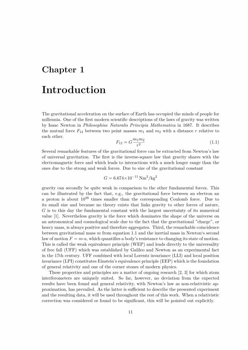
The gravitational acceleration on the surface of Earth has occupied the minds of people formillennia. One of the first modern scientific descriptions of the laws of gravity was writtenby Isaac Newton in Philosophiae Naturalis Principia Mathematica in 1687. It describesthe mutual force F12 between two point masses m1 and m2 with a distance r relative toeach other.
F12 = Gm1m2
r2(1.1)
Several remarkable features of the gravitational force can be extracted from Newton’s lawof universal gravitation. The first is the inverse-square law that gravity shares with theelectromagnetic force and which leads to interactions with a much longer range than theones due to the strong and weak forces. Due to size of the gravitational constant
G = 6.674×10⁻¹¹ Nm2/kg2
gravity can secondly be quite weak in comparison to the other fundamental forces. Thiscan be illustrated by the fact that, e.g., the gravitational force between an electron ana proton is about 1039 times smaller than the corresponding Coulomb force. Due toits small size and because no theory exists that links gravity to other forces of nature,G is to this day the fundamental constant with the largest uncertainty of its numericalvalue [1]. Nevertheless gravity is the force which dominates the shape of the universe onan astronomical and cosmological scale due to the fact that the gravitational ”charge”, orheavy mass, is always positive and therefore aggregates. Third, the remarkable coincidencebetween gravitational mass m from equation 1.1 and the inertial mass in Newton‘s secondlaw of motion F = m·a, which quantifies a body’s resistance to changing its state of motion.This is called the weak equivalence principle (WEP) and leads directly to the universalityof free fall (UFF) which was established by Galileo and Newton as an experimental factin the 17th century. UFF combined with local Lorentz invariance (LLI) and local positioninvariance (LPI) constitutes Einstein’s equivalence principle (EEP) which is the foundationof general relativity and one of the corner stones of modern physics.
These properties and principles are a matter of ongoing research [2, 3] for which atominterferometers are uniquely suited. So far, however, no deviation from the expectedresults have been found and general relativity, with Newton’s law as non-relativistic ap-proximation, has prevailed. As the latter is sufficient to describe the presented experimentand the resulting data, it will be used throughout the rest of this work. When a relativisticcorrection was considered or found to be significant, this will be pointed out explicitly.
11
12 CHAPTER 1. INTRODUCTION
In addition to testing the laws of physics, gravity measurements are also conductedto gain insight into the details of Earth‘s gravitational field. Numerous temporal andspatial changes of the local gravitational acceleration g exist and can be measured withgravimeters to, e.g., draw conclusions on the figure of Earth or geophysical processesunderneath the surface. Most of these variations are significantly smaller than 10−6 g and,for some applications, difficult to measure with current, classical gravimeters.
This thesis is primarily concerned with terrestrial gravity measurements and withthe development and application of a new type of gravimeter using atom interferometryat geodetic observatories. The rest of this chapter will briefly summarize the workingprinciple of a simple atom interferometer and mention the development and applicationsof this research field. Afterwards, some details about Earth’s gravity field with its spatialand temporal variations will be given and the properties of other types of gravimeters willbe discussed briefly. This will be important in order to understand the gravimetric datapresented and the relevance of current and future applications.
1.1 Atom InterferometryThe first atom interferometers were demonstrated in 1991 and 1992 by four differentresearch groups in the United States and Germany around the same time . The firsttwo groups used mechanical, micro-fabricated slits or gratings [4, 5], whereas the othergroups employed the light grating [6, 7] of a laser pulse to induce interference fringesin the detected signals. The experiment described in [7] and shortly after in [8] showedthe first measurements of the gravitational acceleration with atom interferometry. It isbased on stimulated two-photon Raman transitions [9] and its basic working principle isstill the basis for the atomic gravimeter used during this work. The essential mechanismwill therefore be explained here briefly, in addition to the proper theoretical descriptionpresented in chapter 2.
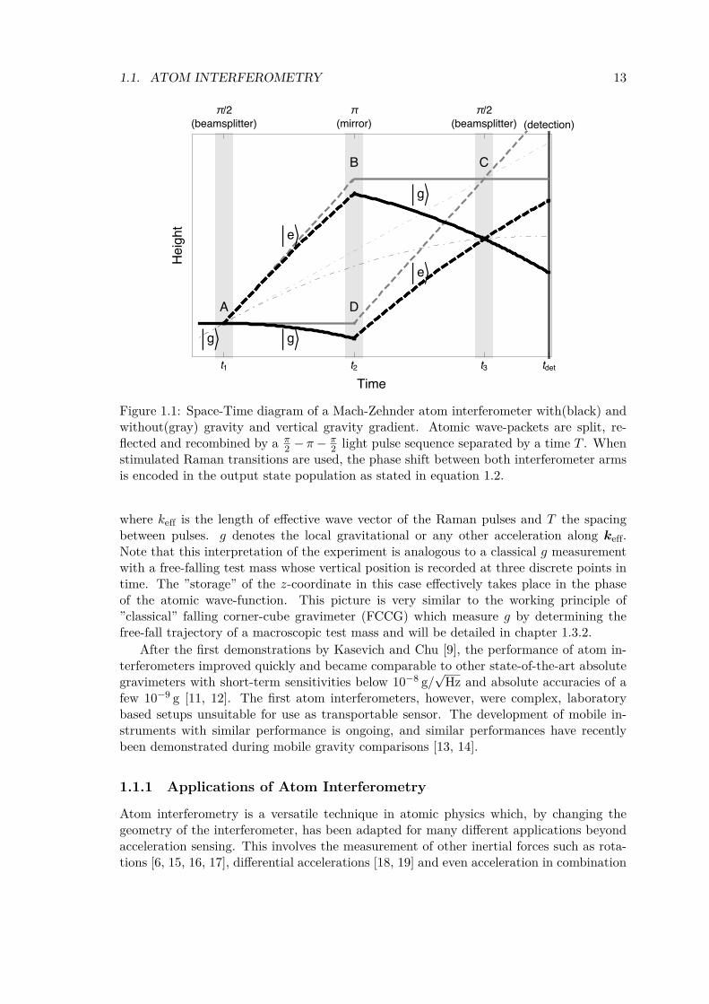
Atoms in an ultra-high vacuum (UHV) chamber are first laser-cooled in a magneto-optical trap (MOT) and subsequent optical molasses to micro-Kelvin temperatures [10]where their wave-like properties start to appear. After releasing the atoms by either simplydropping or launching them upwards using moving molasses, the atomic matter-waves aresplit, reflected and recombined during a so-called π
2 -π-π2 Raman pulse sequence as shownin figure 1.1, where the central pulse is twice as long as the other two pulses. During thistime both interferometer arms are in opposite internal states and separated vertically dueto the photon recoil collected during the state transition. The atomic state populationafter the last pulse then depends on the phase difference ∆Φ accumulated between theupper and lower interferometer paths, resulting in the appearance of interference fringes.For atoms initially in the ground state, the probability of an atom being in the excitedstate after the last pulse is given by
Pe =1
2(1− cos∆Φ) (1.2)
The dominating phase shift in this configuration is caused by the atom-light interactionduring which the local laser light phase is imprinted on the atomic wave function whenevera state transition occurs. When entering the phase at the space-time points A-D asindicated in figure 1.1 and using parabolic atomic trajectories, the phase shift becomes
∆Φ =(ϕA
eff − ϕBeff + ϕC
eff)− ϕD
eff = keffgT2 (1.3)
1.1. ATOM INTERFEROMETRY 13
/( ) ( ) /( ) ( )
Figure 1.1: Space-Time diagram of a Mach-Zehnder atom interferometer with(black) andwithout(gray) gravity and vertical gravity gradient. Atomic wave-packets are split, re-flected and recombined by a π
2 − π− π2 light pulse sequence separated by a time T . When
stimulated Raman transitions are used, the phase shift between both interferometer armsis encoded in the output state population as stated in equation 1.2.
where keff is the length of effective wave vector of the Raman pulses and T the spacingbetween pulses. g denotes the local gravitational or any other acceleration along keff.Note that this interpretation of the experiment is analogous to a classical g measurementwith a free-falling test mass whose vertical position is recorded at three discrete points intime. The ”storage” of the z-coordinate in this case effectively takes place in the phaseof the atomic wave-function. This picture is very similar to the working principle of”classical” falling corner-cube gravimeter (FCCG) which measure g by determining thefree-fall trajectory of a macroscopic test mass and will be detailed in chapter 1.3.2.
After the first demonstrations by Kasevich and Chu [9], the performance of atom in-terferometers improved quickly and became comparable to other state-of-the-art absolutegravimeters with short-term sensitivities below 10−8 g/
√Hz and absolute accuracies of a
few 10−9 g [11, 12]. The first atom interferometers, however, were complex, laboratorybased setups unsuitable for use as transportable sensor. The development of mobile in-struments with similar performance is ongoing, and similar performances have recentlybeen demonstrated during mobile gravity comparisons [13, 14].
1.1.1 Applications of Atom Interferometry
Atom interferometry is a versatile technique in atomic physics which, by changing thegeometry of the interferometer, has been adapted for many different applications beyondacceleration sensing. This involves the measurement of other inertial forces such as rota-tions [6, 15, 16, 17], differential accelerations [18, 19] and even acceleration in combination
14 CHAPTER 1. INTRODUCTION
with magnetic field sensing [20]. The extreme sensitivity to inertial forces can also be em-ployed for the measurement of physical constants such as G [21, 22] or ℏ/m [23]. Usingdifferential atom interferometry, schemes for testing the inverse square law [24] and gen-eral relativity [25] have been proposed. Multi-species atom interferometers have furthertested EEP through the UFF [26]. A comparison of an atomic gravimeter and an FG5 ab-solute gravimeter (AG) presented in [11] was in fact the first UFF test between quantum-and macroscopic particles with a relative uncertainty of a few times 10−9 [27]. This is stillabout four order of magnitude below the bound set by other methods [28] but may beimproved in the future by advanced atom interferometers [29]. Gravitational wave detec-tors based on atom interferometry have also been proposed on earth and in space[30, 31],widening the scope of this technique to the fields of astronomy and astrophysics. Finally,even tests of dark energy due to so-called chameleon fields using atom interferometry havebeen proposed [32, 33].
This list, although far from complete, shows the scope of atom interferometry today inbasic and applied physics, and the generality and flexibility of this method. Geodesy andother Earth sciences provide another wide field of applications which will be detailed inthe following chapters. This work realizes the potential of atom interferometry in this fieldby performing high-precision absolute gravity measurements beyond the state-of-the-artat geodetic observatories and comparing them directly to other types of gravimeters. Inorder to compare the measured signals it is necessary to understand the gravity variationson the surface of Earth. The next chapter will therefore give a brief overview over thisfield.
1.2 Surface Gravity on EarthTo get an understanding of the sources and shape of the expected gravity variationsfound on Earth, this chapter will briefly discuss the models and results describing thegravitational potential and field. Note that this discussion can only be a short overview.A complete description can be found in geodesy textbooks and review articles [34, 35]. Asummary of the most relevant gravity effects is shown in table 1.1.
Earth’s gravity field is the subject of geodesy which is defined according to Helmert[36], as ”... the science of the measurement and mapping of the Earth’s surface.”. Sincethe surface of Earth is, to a large extent, shaped by gravitation, this definition includesthe determination of the Earth’s figure and its external gravity field g(r). Its features arein the following roughly divided into spatial, global and regional gravity effects on onehand and time-dependent effects on the other hand. The former will be described herefirst. After covering the basic definitions, temporal gravity changes are discussed in thefollowing chapters.
In order to simplify the mathematical description we write the conservative gravityfield g it in terms of its scalar potential W so that g = −gn = ∇W with the upwardspointing unit vector n. By convention, the centrifugal acceleration due to Earth’s rotationis already incorporated into the potential, yielding [34]
W (r) = V (r) + Z(p) = G
∫Earth
ρ(r′)
|r − r′|d3r′ +
Ω2E
2p2 (1.4)
where V denotes the gravitational potential of Earth without rotation defined by its densitydistribution ρ. Z gives the centrifugal potential depending on the distance from the
1.2. SURFACE GRAVITY ON EARTH 15
90°
60°
30°
-30°
0°
0°
-60°
-90°30° 60° 90° 120° 150° 180° 210° 240° 270°
mGal
300° 330° 360°
100 90 80 70 60 50 40 30 20 10 0
-10-20-30-40-50-60-70-80-90
-100
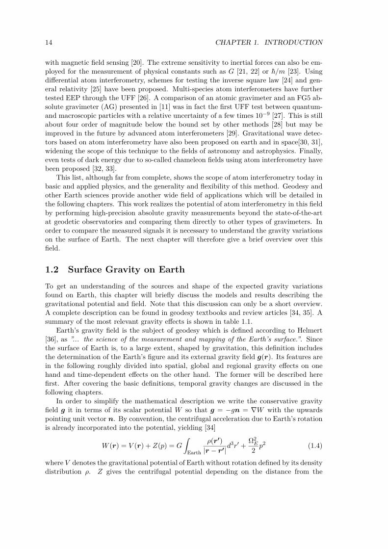
Figure 1.2: Free-air gravity anomalies ∆g derived from the EGM08[37] model, combiningthe satellite ITG-GRACE03s [38] gravitational model with terrestrial, altimetry-derivedand airborne gravity data
(1 mGal = 10−6 g
). Figure from [39]
rotation axis p = R cos(θ), where θ is the geographical latitude and R is the radiusof Earth. The first term gives as a first, crude, approximation for a spherical Earth,with GM = 398.6×10¹² m3/s2 and R = 6371 km a potential V = 6.26×10⁷ m2/s2 andgravitational acceleration 9.82 m/s2 on Earth’s surface. The rotation superimposes theadditional centrifugal acceleration Ω2
Ep ≤ 0.03 m/s2. This causes the flattening of Earth,giving it its ellipsoidal shape and a gravity value of around 9.78 m/s2 at the equator and9.83 m/s2 at the poles. Note that, throughout this work, relative quantities or SI unitswere used for g whenever possible. When citing existing literature, however, the older butstill widely used Gal is sometimes used: 1 Gal = 10−2 m/s2 ≈ 10−3 g.
Local features and anomalies of Earth’s gravity field are contained in the geoid whichwas introduced in 1828 by C.F. Gauss [34] as the “equipotential surface of the Earth’sgravity field coinciding with the mean sea level of the oceans”, or W (r) = W0. If thedensity distribution ρ inside the earth was fully known, the gravity potential and the geoidW0 could be calculate with equation 1.4. Unfortunately, accurate density measurementsare only available for the upper layers of Earth [34]. Gravity observation therefore have tobe used to construct a model which is usually expressed as a spherical harmonic expansion[34]. Figure 1.2 shows a global model of Earth‘s gravitational field compiled from amultitude of gravity observations. The free-air anomalies ∆g denote the difference betweenthe measured surface gravity value gP and the calculated value at normal height1 HN
above the ellipsoid, so thatgP = g0 + γ ·HN +∆g (1.5)
where g0 is the calculated normal gravity value on the ellipsoid surface [34]. The verticalfree-air gravity gradient γ := ∂rg can for this purpose be approximated by a mean valueof γ ≊ −3086 nms−2/m. Note that the geoid height itself is related to the shown gravity
1More specifically, HN gives the height above the ellipsoid with normal potential equal to the surfacepotential at point P (telluroid). See also [34], chapter 6.
16 CHAPTER 1. INTRODUCTION
Moon
Earth
rm
lm= r-rmr
0a0
a0
a
aat
ψ
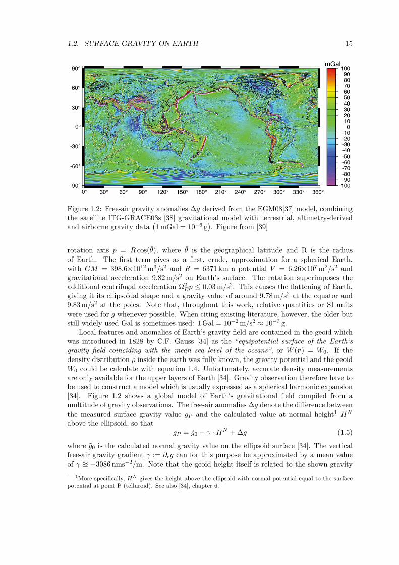
Figure 1.3: Basic tidal acceleration at of the moon according to equation 1.6, shownas gray arrows. A bulge forms on the front- and back-facing sides causing semi-diurnalgravity variations. The gray elliptic surface indicates the vertical shift of a level surfaceby the tidal potential Vt.
anomalies and derived from the same model [37]. Figure 1.2 shows many regional andlocal anomalies with a magnitude of 10−6–10−4 g. Geographic features such as mountains,ocean as well as tectonic or other geophysical influences such as ocean trenches and platetectonics are clearly visible.
The shown model is complete to spherical harmonic coefficients to degree and order2159. The satellite data only contributes to degree 360 while the higher frequency com-ponents are only possible by combining this with terrestrial gravity data.
1.2.1 Tidal Gravity VariationsIn addition to the more or less static local, regional and global structure described above,the gravitational field at a fixed location is also time-dependent. Although much smallerat a maximum size of around 10−7 g, temporal gravity effects are actually more relevantfor this work which is concerned with gravity observations conducted over several daysor weeks at one given measurement site. The largest effect is given by the gravitationof sun and moon, the other planets in the solar system contribute on a much smallerscale. These lunisolar accelerations result in the basic tidal effect on earth which willbe summarized below for the two-body problem Earth-Moon. Consider a non-rotatinggeocentric coordinate system in which all points experience the same orbital accelerationa0 due to the movement around the barycenter of the Earth-Moon system. At Earth’scenter of mass, a0 and the gravitational force a cancel out whereas all other points on Earthare subject to tidal forces at. When applying Newton’s law of gravitation as illustratedin figure 1.3, one obtains:
at = a− a0 =GMm
l2m
lmlm
− GMm
r2m
rmrm
(1.6)
where rm is the distance between both center of masses and lm := |r−rm| is the local dis-tance to the moon. These tidal forces deform Earth’s gravity field which, in a coordinatesystem fixed to its surface, cause the diurnal and semi-diurnal tidal gravity variations. Inorder to simplify the calculations it is again useful to transition from the tidal acceleration
1.2. SURFACE GRAVITY ON EARTH 17
-
-
-
µ/
Figure 1.4: Continuous gravity registration of the atomic gravimeter GAIN over a periodof several days during the comparison campaign in Wettzell, Bavaria, demonstrating theeffect of tidal gravity changes. Each data point represents the mean-value for 10 min ofdata.
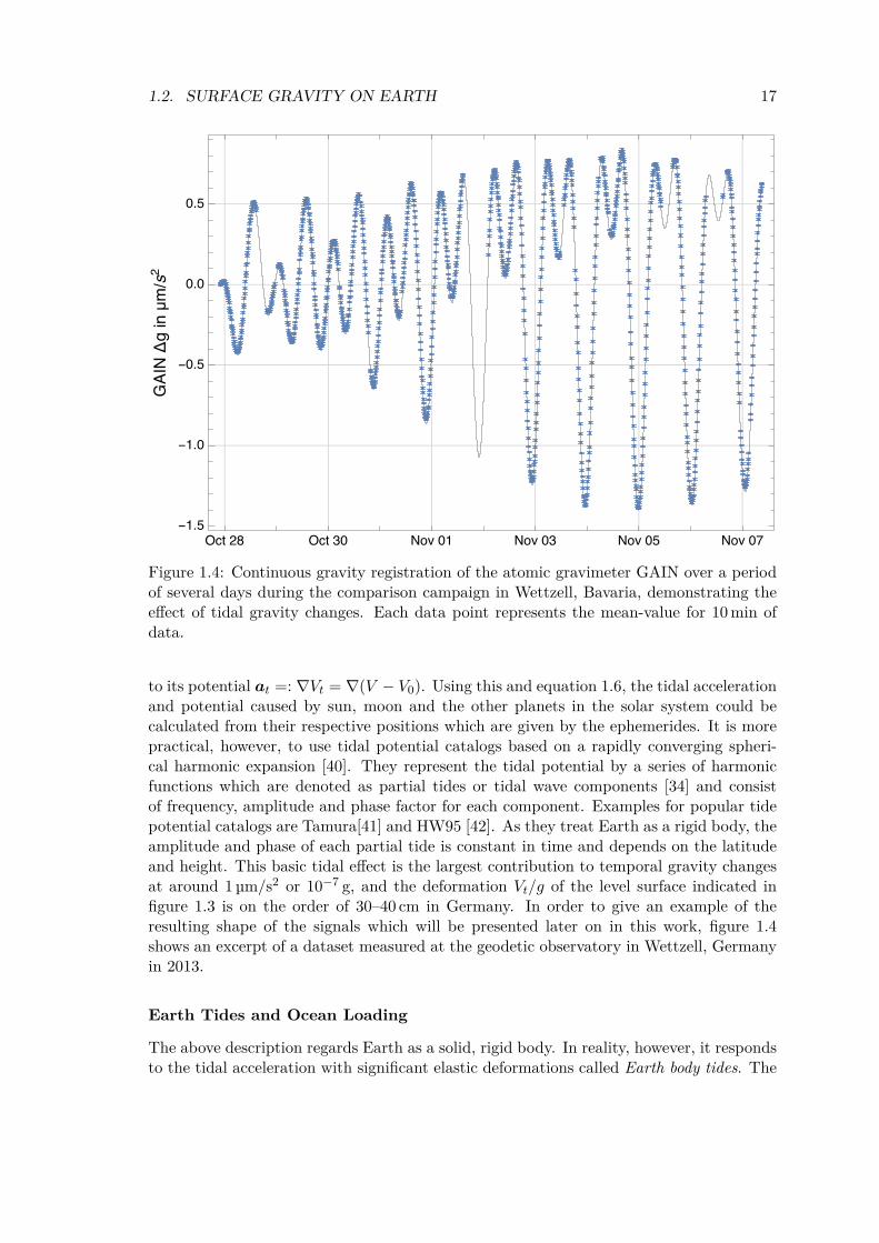
to its potential at =: ∇Vt = ∇(V − V0). Using this and equation 1.6, the tidal accelerationand potential caused by sun, moon and the other planets in the solar system could becalculated from their respective positions which are given by the ephemerides. It is morepractical, however, to use tidal potential catalogs based on a rapidly converging spheri-cal harmonic expansion [40]. They represent the tidal potential by a series of harmonicfunctions which are denoted as partial tides or tidal wave components [34] and consistof frequency, amplitude and phase factor for each component. Examples for popular tidepotential catalogs are Tamura[41] and HW95 [42]. As they treat Earth as a rigid body, theamplitude and phase of each partial tide is constant in time and depends on the latitudeand height. This basic tidal effect is the largest contribution to temporal gravity changesat around 1 µm/s2 or 10−7 g, and the deformation Vt/g of the level surface indicated infigure 1.3 is on the order of 30–40 cm in Germany. In order to give an example of theresulting shape of the signals which will be presented later on in this work, figure 1.4shows an excerpt of a dataset measured at the geodetic observatory in Wettzell, Germanyin 2013.
Earth Tides and Ocean Loading
The above description regards Earth as a solid, rigid body. In reality, however, it respondsto the tidal acceleration with significant elastic deformations called Earth body tides. The

18 CHAPTER 1. INTRODUCTION
total potential change ∆V at the surface of Earth therefore consists of the direct per-turbation Vt superimposed with a potential change due to the tidal induced mass shiftand the potential change caused by the vertical shift of the surface [34]. The latter twocontributions can be described empirically using gravimetric amplitude and phase factorsδi, ∆φi for each partial tide i. The measured gravity variations including these effects arethen given by the observation equation [34]
gel(t) =∑i
δiAtheoi cos
(ωit+ φtheo
i +∆φi
)(1.7)
δi :=Aobsi /Atheo
i ∆φi := φobsi − φtheo
i (1.8)(1.9)
where gel(t) is the observed change at a given point on the surface of Earth including theelastic response and ωi, Atheo
i , φtheoi denote the calculated values for the respective partial
tide from e.g. a tidal potential catalog. To first order, Earth tides can be described usingthe theoretically derived Love numbers [43] resulting in an amplitude factor of δ = 1.16.Note that measured gravity changes which include the elastic response are therefore about16 % larger than the modeled tides on the rigid Earth. Because the resonance frequencyof the elastic Earth is far below the dominating semi-diurnal and diurnal partial tides, theassociated phase shift vanishes in this case.
Similar to Earth tides, shifting water and atmospheric masses and the associated heightchanges due to loading effects perturb the tidal gravity potential and are referred to astidal loading. Contrary to the elastic response of Earth, however, the oscillation periodsof ocean tides depend strongly on the topography of the sea floor and the coastline.The phase factors associated with ocean loading therefore vary significantly from zeroand are strongly position dependent. The amplitude of the ocean loading also dependsstrongly on the distance to the coastline and can reach the same magnitude as Earth tides.Atmospheric loading effects due to the solar heating and associated pressure oscillationsalso have a tidal component which is, however, one order of magnitude smaller than Earthtides and ocean loading [34].
Detailed synthetic models of both earth tide and ocean loading have previously beenpublished and combined in order to calculate worldwide synthetic tide models [44, 45,46] which provide accurate gravimetric reductions on the 10−9 g level except for locallydisturbed coastal and polar regions. Alternatively, models which are restricted to a certainmeasurement site can be derived from continuous gravity observations over periods longerthan the respective partial tide period. Depending on the stability of the instrumentand length of the dataset, up to 40 partial tides can be resolved this way with currentsuperconducting gravimeters [34]. Further advantages and limitations of this approach arerelated to the instrumental properties of currently used gravimeters and will be discussedin detail in chapter 1.3.
All tidal models used throughout this work are presented in Appendix B and includetidal and ocean loading in terms of amplitude and phase factors. The denoted frequencyrange of each wave group contains a number of partial tides. Gravity predictions werederived from the model using the program Tsoft [47] which uses the tidal potential catalogby Tamura containing 1200 partial tides [41].
1.2. SURFACE GRAVITY ON EARTH 19
1.2.2 Atmospheric Pressure VariationsThe local gravity value is strongly correlated with air-pressure due to the direct attractionof the air and the atmospheric loading similar to the effects described in the previouschapter. Their combined effect can be estimated and removed from gravity time-seriesreasonably well using the simple reduction [48]
∆gatm = ap (p(t)− p0) (1.10)
where ap ≈ 3 nm/s2/hPa [49, 50] is the pressure admittance factor which can vary slightlybetween measurement sites, p(t) is the local time-variable air pressure and p0 is the heightdependent base pressure according to the barometric formula B.1. Equation 1.10 onlyaccounts for about 95 % of the total atmospheric effect. More sophisticated models [51,52] are available which calculate the direct attraction using a 3D density distribution ofthe atmosphere over a larger area around the measurement sites from weather models.For the purpose of this work, however, the simple reduction formula 1.10 proved sufficient.
1.2.3 Polar MotionEarth’s rotational vector ΩE is subject to periodic and irregular changes which are mon-itored with high precision through space geodesy methods such as VLBI. The horizontalmovement of the pole coordintates leads to variations in the centrifugal acceleration z.The associated gravity effect can be calculated using the formula [53]
∆gpol = −δ · Ω2ER sin 2θ (xpol cosλ− ypol sinλ) (1.11)
with the geographical latitude θ and longitude λ of the measurement position and the ap-proximate amplitude factor δ introduced in chapter 1.2.1 accounting for Earth’s elasticity.(xpol, ypol) are daily pole coordinates with respect to the IERS reference pole [54]. Pre-dicted values are available for analysis during a measurement campaign and final valueswith a high accuracy for post-processing. The magnitude of ∆gpol is usually smaller than10−8 g and can, due to the high accuracy of the Earth orientation parameters, be reducedto less than 10−10 g [34]. During this work an existing implementation of equation 1.11 inthe program Tsoft was used.
1.2.4 HydrologyAfter applying an accurate tidal model which includes loading effects and accounting foratmospheric pressure and polar motion corrections, the residual gravity signal at mostmeasurement sites has a magnitude in the low 10−9 g range. The remaining part is usuallycaused by non-tidal environmental mass redistributions such as changes in the local watertable due to precipitation and other climate effects. The associated effect is dominated bydirect attraction and could in principle be approximated to first order by using a similarmethod chosen for air pressure correction [53]. This method is, however, restricted toregions with homogeneous sediment layers and handicapped by missing data on the localor regional hydrology. It therefore constitutes one of the least well modeled signals interrestrial gravity monitoring [55] with a magnitude of 10−10–10−9 g over days and up to10−8 g for longer data sets during seasonal changes which can be ascribed to total waterstorage dynamics. This is an important application of superconducting gravimeters asmentioned in chapter 1.3.3.
20 CHAPTER 1. INTRODUCTION
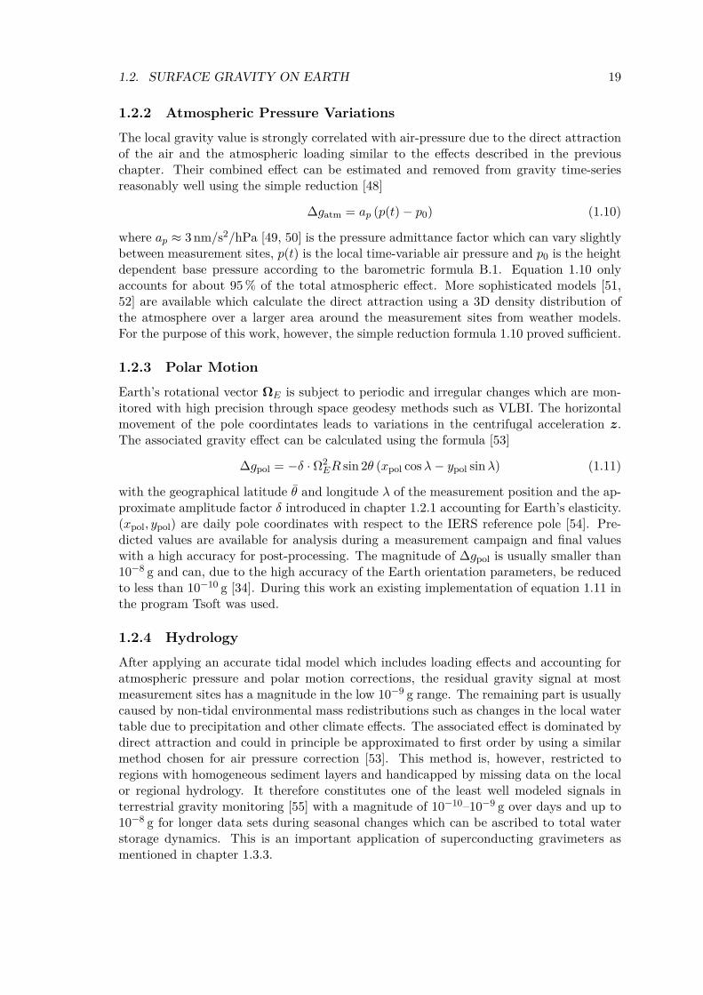
Effect description Magnitude TimescaleGeographicalGlobal Scale 10−3 gRegional Scale 10−4–10−6 g constantFree-air gravity gradient −3×10⁻⁷ g/mTidalDirect Lunisolar Gravitation 10−7 g
6 h - yearsEarth Tides 10−8 gOcean Loading 10−8 gAtmospheric Loading 10−9 gEnvironmentalAtmospheric Pressure −3×10⁻¹⁰ g/hPa hours - daysWater Table / Hydrology 10−8–10−10 g days - seasonalAstronomical & GeophysicalPolar Motion ≤ 10−8 g weeks - secularGlacial Isostatic Adjustment 10−9 g/year secularTectonic Plate Movement 10−9 g/yearVolcanology 10−10–10−7 g secular, sudden eventsEarthquakes, Seismic Modes 10−10–10−9 g
Table 1.1: Overview of temporal and geographical gravity changes on the surface of Earth.(1 µGal = 10 nm/s2 ≈ 10−9 g). Refer to [34, 35] for a more detailed description.
1.3 Terrestrial GravimetryToday, no single type of gravimeter can fulfill the requirements for all applications and thedifferent instruments often have to be used in combination to obtain the required gravitydata. This is a direct consequence of the technological limitations of their respectivemeasurement principles which will be discussed below. Atom interferometers such as thegravimetric atom interferometer (GAIN) presented here show the potential to alleviatethis situation and combine the advantages of the different gravimeter types into a singleinstrument. This will reduce both the effort needed in acquiring this data and improve itsquality due to reduced instrumental uncertainties.
This chapter attempts to give an overview of the working principles as well as theadvantages and drawbacks of the current, classical types of gravimeters. Based on theseproperties their various applications in geodesy and related fields will then be highlightedin chapter 1.3.3 in order to identify the areas where atomic gravimeters can benefit currentand future applications most.
Two different sorts of instrument have been developed for generating gravity data, rel-ative and absolute gravimeters. The former only record differences between gravity valuesduring continuous registrations or transport and need to be calibrated against a knowngravimetric standard in order to relate their output to physical gravity signals. Absolutegravimeters (AGs), on the other hand, obtain the full value of g by referencing the freefall acceleration of a test mass to a time and length standard. Within the accuracy limitsof those underlying standards no calibration is necessary which, in principle, makes this

1.3. TERRESTRIAL GRAVIMETRY 21
m
mg
k(l-l0) m
mg
k(l-l0)
α
δ
a
h
b
d
Figure 1.5: Operating principle of vertical spring (left) and general lever spring balancegravimeter (middle), from [56]. Microg-LaCoste gPhone (right) in operation with elec-tronics and sensor head (bottom right). Image courtesy of M. Schilling, IfE Hannover.
type of instrument more attractive for many applications. Practically, however, the tech-nical limitations of current state-of-the-art instruments require both types of instrumentsto cover the whole spectrum of applications in Earth sciences. In order to put the grav-ity comparisons between GAIN and other state-of-the-art gravimeters into context it istherefore relevant to understand their instrumental differences.
1.3.1 Relative Gravimeters
Within this section, again two main categories exist: spring-type and superconductinggravimeters. Both are based on measuring the gravitational force on a vertically suspendedoscillatory system and will be described here briefly. Refer to [34, 35] for more details.
Spring Gravimeters
Spring gravimeters are based on a test mass m, suspended against gravity with a verystable mechanical spring of initial length l0 as shown in figure 1.5. For the simple verticalspring system, changes in g can then be measured simply by monitoring the length of thespring which is governed by Hooke’s law, yielding
g =k
m(l − l0) (1.12)
where k is the spring constant. The mechanical sensitivity ∂gl = m/k = ω−20 is problem-
atically low for vertical spring gravimeters, requiring a mass position readout precision oftypically less than 1 nm for a gravity change of 10−8 g for realistic resonance frequencies[53]. Nevertheless this principle is successfully employed in Scintrex gravimeters due toits robustness and compact size.
In order to improve the intrinsic sensitivity and relax the readout system requirements,LaCoste-Romberg (LCR) type lever spring balance systems [57] were developed. Theequilibrium condition for the torques as shown on the right side of figure 1.5 reads
mg sin (α+ δ) = k (l − l0)h = k (l − l0) bb
lsinα (1.13)

22 CHAPTER 1. INTRODUCTION
The associated sensitivity in this configuration is given by
dα
dg=
sin (α+ δ) sinα
g sin δ(1.14)
which becomes large for small δ and α ≈ 90 °. The sensitivity improvement compared to avertical spring is about three orders of magnitude which results in only µm level readoutprecision requirements. Examples for LCR instruments are the ZLS Burris or the Microg-LaCoste gPhone gravimeter, see also [58]. The gPhone which is depicted in figure 1.5 wasalso present for the first gravity comparison campaign shown in chapter 5. In order toreduce the influence of thermal expansion and other systematic effects, the spring-masssystem of all modern spring gravimeters is housed in a hermetically sealed casing withtemperature- and pressure stabilization as well as magnetic shielding. In order to suppressnon-linearities of the mechanical system and extend the dynamic range of the instrument,electronic feedback systems keep the mass at the zero position during gravity changes byapplying an additional feedback force. The output signal in this closed-loop configurationis then given by the amplitude of the feedback error signal. The long-term stability ofthe spring, which is usually made from NiFe alloys LCR or fused silica (Scintrex), is acritical parameter for these instruments. Despite considerable optimization efforts, driftsof several 10−8 g/day remain and have to be removed in post-processing on a best-effortbasis which severely limits the range of applications.
In order to relate the output signal to physical gravity changes, a calibration functionfor these instruments is usually determined through relative measurements on calibrationlines, controlled environments with significant gravity differences that were previouslycharacterized using absolute gravimeters.
Superconducting Gravimeters
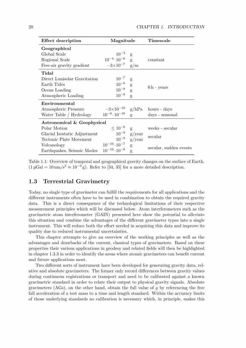
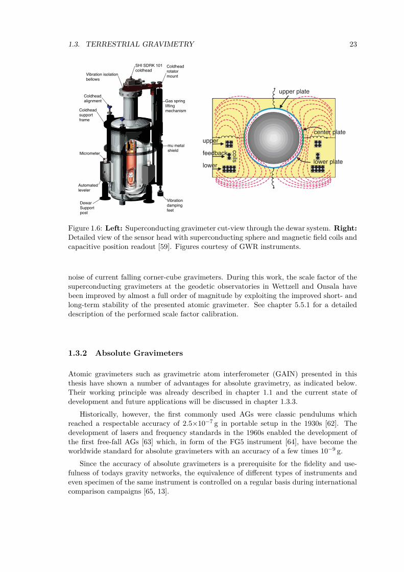
In order to overcome the drift limitations of spring gravimeters, superconducting gravime-ter (SCG) were developed [60]. Their basic idea is to replace the mechanical spring witha permanent current through a superconducting coil pair. The test mass is facilitatedby a superconducting sphere levitating in the associated magnetic field, with its positionmonitored by a capacitive bridge as depicted in figure 1.6. The current difference be-tween the upper and lower field coils is carefully tuned in order to create a field gradientwhich results in a shallow potential and large vertical sphere displacements during gravitychanges. An additional feedback coil applies a correcting force to zero the sphere positionwithin the loop bandwidth. Due to the superconducting, cryogenic system without ohmicresistance, the drift rate of these systems can be as low as 10−11 g/day when operatingcontinuously over several years at a fixed measurement site. The noise level is lower thanany other type of instrument’s and can reach down to only a few nm/s2/
√Hz. In addition
to previous observatory instruments, portable SCG have recently become available [61].Due to the more complex setup and the fact that gravity comparison between sites maybe subject to significant flux jumps, the predominant use of SCGs lies in stationary, longterm gravity observations.
Just like any relative gravimeter, the calibration factors of SCGs need to be determinedwith respect to a known gravity difference. For SCG this is usually done through simul-taneous absolute gravimeter measurements by exploiting the tidal gravity signal. Thismethod, however, is limited to a calibration error of around 10−3 due to measurement
1.3. TERRESTRIAL GRAVIMETRY 23
upper plate
upper center plate
lower platelower
feedback
coils
Gas springliftingmechanism
Coldheadrotatormount
mu metalshield
Vibrationdampingfeet
DewarSupportpost
Automatedleveler
Micrometer
Coldheadsupportframe
Coldheadalignment
Vibration isolationbellows
SHI SDRK 101coldhead
Figure 1.6: Left: Superconducting gravimeter cut-view through the dewar system. Right:Detailed view of the sensor head with superconducting sphere and magnetic field coils andcapacitive position readout [59]. Figures courtesy of GWR instruments.
noise of current falling corner-cube gravimeters. During this work, the scale factor of thesuperconducting gravimeters at the geodetic observatories in Wettzell and Onsala havebeen improved by almost a full order of magnitude by exploiting the improved short- andlong-term stability of the presented atomic gravimeter. See chapter 5.5.1 for a detaileddescription of the performed scale factor calibration.
1.3.2 Absolute Gravimeters
Atomic gravimeters such as gravimetric atom interferometer (GAIN) presented in thisthesis have shown a number of advantages for absolute gravimetry, as indicated below.Their working principle was already described in chapter 1.1 and the current state ofdevelopment and future applications will be discussed in chapter 1.3.3.
Historically, however, the first commonly used AGs were classic pendulums whichreached a respectable accuracy of 2.5×10⁻⁷ g in portable setup in the 1930s [62]. Thedevelopment of lasers and frequency standards in the 1960s enabled the development ofthe first free-fall AGs [63] which, in form of the FG5 instrument [64], have become theworldwide standard for absolute gravimeters with an accuracy of a few times 10−9 g.
Since the accuracy of absolute gravimeters is a prerequisite for the fidelity and use-fulness of todays gravity networks, the equivalence of different types of instruments andeven specimen of the same instrument is controlled on a regular basis during internationalcomparison campaigns [65, 13].
24 CHAPTER 1. INTRODUCTION
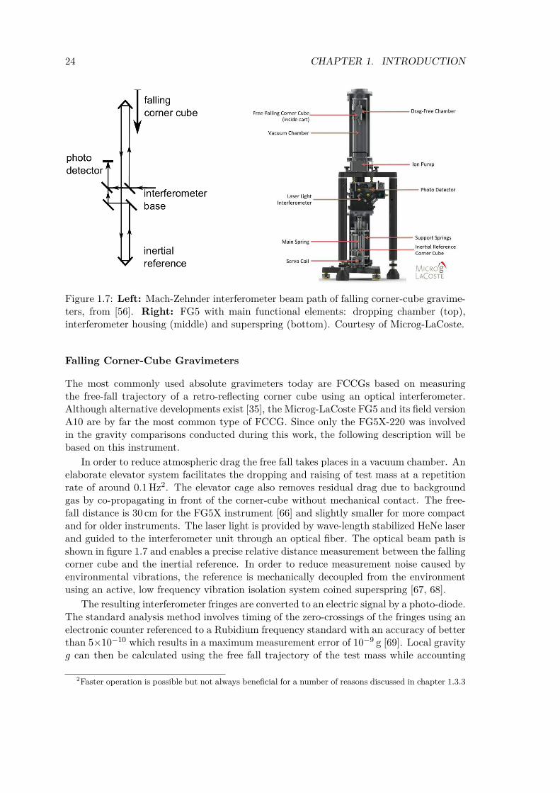
Figure 1.7: Left: Mach-Zehnder interferometer beam path of falling corner-cube gravime-ters, from [56]. Right: FG5 with main functional elements: dropping chamber (top),interferometer housing (middle) and superspring (bottom). Courtesy of Microg-LaCoste.
Falling Corner-Cube Gravimeters
The most commonly used absolute gravimeters today are FCCGs based on measuringthe free-fall trajectory of a retro-reflecting corner cube using an optical interferometer.Although alternative developments exist [35], the Microg-LaCoste FG5 and its field versionA10 are by far the most common type of FCCG. Since only the FG5X-220 was involvedin the gravity comparisons conducted during this work, the following description will bebased on this instrument.
In order to reduce atmospheric drag the free fall takes places in a vacuum chamber. Anelaborate elevator system facilitates the dropping and raising of test mass at a repetitionrate of around 0.1 Hz2. The elevator cage also removes residual drag due to backgroundgas by co-propagating in front of the corner-cube without mechanical contact. The free-fall distance is 30 cm for the FG5X instrument [66] and slightly smaller for more compactand for older instruments. The laser light is provided by wave-length stabilized HeNe laserand guided to the interferometer unit through an optical fiber. The optical beam path isshown in figure 1.7 and enables a precise relative distance measurement between the fallingcorner cube and the inertial reference. In order to reduce measurement noise caused byenvironmental vibrations, the reference is mechanically decoupled from the environmentusing an active, low frequency vibration isolation system coined superspring [67, 68].
The resulting interferometer fringes are converted to an electric signal by a photo-diode.The standard analysis method involves timing of the zero-crossings of the fringes using anelectronic counter referenced to a Rubidium frequency standard with an accuracy of betterthan 5×10⁻¹⁰ which results in a maximum measurement error of 10−9 g [69]. Local gravityg can then be calculated using the free fall trajectory of the test mass while accounting
2Faster operation is possible but not always beneficial for a number of reasons discussed in chapter 1.3.3
1.3. TERRESTRIAL GRAVIMETRY 25
for the vertical gravity gradient γ
z(t) = −g02t2 + v0t− z0 + γt2
(− 1
24g0t
2 +1
6v0t+
1
2z0
)+O(γ2) (1.15)
where g0 := g(z = 0) and z0, v0 are the initial position and velocity of the test mass. Thespecified performance of the state-of-the-art FG5X instrument under optimal conditionsis given by 150 nm/s2/
√Hz and an absolute accuracy of 20 nm/s2. During international
comparisons, the results of different instruments are consistent within 20–50 nm/s2 [65,13].
Typical operation during an FG5 gravity measurement involves performing around 100dropping experiments per hour with an interval of 10 s between drops for around 8-10 hoursduring a period of low micro-seismic vibrations in order to minimize measurement noise[69]. For the rest of the time the device rests in order to minimize mechanical wear andtear. This is repeated around 3-4 times, potentially while repeating the set-up procedurewith different device orientations in order to prevent set-up dependent systematics [14,70].
1.3.3 Applications of Current and Future GravimetersThis subchapter summarizes the typical use cases of the above mentioned types of gravime-ters which are closely connected to their technical strengths and limitations. The resultingpicture is then used to motivate the use of atomic gravimeters in geodesy and geophysics.Starting from their current state of development, this constitutes the main idea behindthis thesis which will be summarized.
FG5 or other FCCG absolute gravimeters are most often used for gravity point mea-surements which, e.g., implement reference sites as part of gravity networks. When re-peated periodically, FG5 measurement have also been used to investigate secular geophys-ical processes such as post-glacial rebound [71]. Relative gravimeters are unsuitable forthis purpose as the small amplitude and rate of change would make it almost impossibleto distinguish the desired gravity signal from instrumental drift. The mechanical wear andtear and the comparatively large measurement noise of FCCG, on the other hand, makethem unsuitable for continuous operation over extended periods of time.
Relative spring gravimeters are, due to their portability and cost effectiveness, of-ten employed to lay out local gravity networks for geophysical monitoring or to increasethe density of absolute gravity networks. They are furthermore used to support absolutegravity measurements through the determination of vertical and horizontal gradients. Ad-ditionally, long-term gravity registrations over several weeks or months for, e.g. tide modelcharacterizations can be carried out using LCR spring gravimeters. Here the instrumentaldrift unfortunately prevents the study of slow gravity changes in the 10−9 g range due towater table fluctuations or other environmental mass redistributions. Superconductinggravimeters have in the past been used for long-term gravity observations over years oreven decades [35] in permanent installations. Their small and very linear drift enablesinvestigations of hydrological and geophysical gravity signal in the 10−10 g range not pos-sible with spring-type instruments. More recently a portable SCG instrument has beendeveloped [61, 72] with similar performance, extending the reach for these instrumentsbeyond geodetic observatories. This instrument has, for instance, been used successfullyto monitor local water storage variations under field conditions [73]. Despite the vast
26 CHAPTER 1. INTRODUCTION
improvement compared to spring gravimeters, SCG data are still subject to instrumen-tal drift of several 10−9 g over a number of years which is large enough to mask secularsignals of geophysical origin such as plate tectonics of post-glacial rebound. Comparisoncampaigns involving FCCG are therefore required on a regular basis for drift determi-nation which introduces uncertainties in the 10−9 g level due to error in the FG5 pointmeasurements [35] and significantly increases the cost and effort needed for drift-free con-tinuous gravity data. Atomic gravimeters, on the other hand, enable long-term absolutegravity monitoring with a stability in or below the 10−9 g range as shown in this work.This would be highly beneficial for a these and related applications in geodesy, geophysicsand hydrology.
Another practical consideration is the range of available measurement sites. FG5absolute gravimeters are only employed on a solid concrete foundation in order reduce self-induced vibration due to the moving test-mass. They also exhibit increased measurementnoise in the presence of elevated micro-seismic vibrations caused by, e.g., stormy and windyweather conditions or human activity. Both factors strongly restrict the availability ofmeasurement sites for absolute gravimetry. Atom interferometers have shown the potentialto relax these restrictions of currently used absolute and relative gravimeters. As they donot rely on moving parts and operate with a high repetition rate, they offer the prospect ofcontinuous absolute measurements with high long- and short-term stability in the 10−9 gor better while being less sensitive to environmental noise.
Most of the atomic gravimeters developed to date, however, were realized as large,stationary, experimental setups unsuitable for field use [27, 12] and the development ofcompact, portable and robust field instruments is still in progress today [14, 74]. Althoughthe first commercial atomic gravimeters have recently become available [75, 76, 77], theiradaption in geodesy and specific other earth sciences is still in its infancy and their exactperformance not yet fully known.
The underlying goal of the presented work is therefore to make a state-of-the-art atomicgravimeter available for geodetic applications and exploit the potential of this new classof sensors under realistic conditions during measurement campaigns at several geodeticsites. This was demonstrated specifically by conducting state-of-the-art absolute gravitymeasurements outside of the laboratory at geodetic observatories in Wettzell, Germanyand Onsala, Sweden with the Gravimetric atom interferometer (GAIN) at Humboldt Uni-versität zu Berlin (HUB). A comparison to other state-of-the-art absolute and relativegravimeters was carried out during each campaign in order to distinguish instrumentaleffects from real gravity changes and demonstrate the benefits of this new kind of sensorfor the above-mentioned applications. Before conducting these measurements the per-formance, mobility and robustness of the atom interferometer setup was improved andverified during test measurements in Berlin.
1.4 Thesis Structure
After reviewing the objective framework, chapter 2 will review the theoretical description ofthe atom interferometer. The following chapters 3 and 4 describe the experimental setupand the measurement sequence which was used for the gravity comparison campaigns.Special emphasis here is put on the parts to which the author contributed most duringthe work on the setup, namely the vibration isolation and Coriolis compensation setup,
1.4. THESIS STRUCTURE 27
RF frequency control system and improvements on the atomic source. Chapter 5 includesa detailed analysis of the gravity data obtained during all four gravity campaigns witha quantitative comparison to the other gravimeters types. This includes the achievedGAIN measurement noise, long-term stability and the absolute accuracy. Chapter 6 givesa detailed account of the systematic effects and error budget that were investigated duringthis work. The conclusion explores the implications of the presented results. An outlookon current and future benefits of atom interferometry for the field of gravimetry both ingeodetic observatories and other environments will be derived.

28 CHAPTER 1. INTRODUCTION
Chapter 2
Theory
In order to realize gravimetric measurements with the desired accuracy, the gravity inducedatom interferometer phase ∆Φ needs to be known, including higher-order corrections. Thisderivation summarizes the important results in a self-contained manner and refers to theextensive existing literature on light-pulse atom interferometers where appropriate.
First, the atom-light interaction during stimulated, two-photon Raman transition isintroduced which causes the dominating phase contribution. The complete interferometerphase will then be derived using the path integral method including higher order cor-rections due to gravity gradients. Finally, the sensitivity function of Mach-Zehnder atominterferometers is used to derive the effect of finite-length Raman pulses and Raman phasenoise.
2.1 Stimulated Raman TransitionsThe interferometer sequence described later in this chapter infers transitions between twointernal atomic states, |g⟩ and |e⟩, which have to be stable enough to neglect spontaneousdecay within the time scale of the experiment. One good candidate are the hyperfine statesof Alkali metals such as Rubidium with transition frequencies in the radio frequency (RF)range. As will become clear later, the sensitivity of the interferometer phase to inertialforces scales linearly with the Doppler shift ∆ω = k · v of the transition frequency, wherek is the light‘s wave vector and v the atomic velocity . In order to increase the sensitivityit is beneficial to make k larger by not driving the RF transition directly, but employingtwo-photon Raman transitions via an intermediate state |i⟩ using counter-propagationbeams as depicted in figure 2.1. This results in a Doppler sensitivity of ∆ω = keff · v, withthe effective wave vector
keff := k1 − k2 = (|k1|+ |k2|) ek
For 87Rb, Doppler sensitive Raman transitions via the D2 line lead to keff ≊ 1.61×10⁷ m−1
compared to kRF ≈ 143 m−1 when driving the transition directly using a 6.8 GHz micro-wave, a gain of five orders of magnitude. The description of the atom-light interactiongiving here follows a treatment from [78] and briefly outlines intermediate and main resultsof the calculation.
Both the internal state of a three-level system and the external momentum of theatomic wave-packet need to be considered. The latter can be conveniently describe as a
29

30 CHAPTER 2. THEORY
p = 0
p = 0
Final
Initial
p = ħ(|k1|-|k2|)
ħ(k1+k2)
Final
Initial
e
e
g
g
p = ħkeff = ħ(|k1|+|k2|)2ħk2
2ħk2
ħk2ħk1
Doppler Insensitive
Doppler Sensitive
|g⟩
|i⟩
|e⟩ω1
ω2
ω2
ω1∆
δ
ωeg
∆2g
∆1e
Figure 2.1: Left: Stimulated Raman transitions and momentum recoil for Doppler sensi-tive (counter-propagating) and insensitive (co-propagating) beam configurations. Right:Three-level system and Raman driving fields ω1/2 with one- and two-photon detunings ∆and δ. The dotted off-resonant transitions cause additional AC-stark offsets.
sum of momentum plane-wave states |p⟩ and the internal atomic states |g⟩ , |e⟩ , |i⟩ and bewritten as the tensor product of two Hilbert spaces
|g,pg⟩ = |g⟩ ⊗ |pg⟩|e,pe⟩ = |e⟩ ⊗ |pe⟩|i,pi⟩ = |i⟩ ⊗ |pi⟩
The Hamiltonian for this problem is given by [78]:
H =p2
2m+ ℏωg |g⟩ ⟨g|+ ℏωe |e⟩ ⟨e|+ ℏωi |i⟩ ⟨i|︸ ︷︷ ︸
=:H0
− d · E︸ ︷︷ ︸=:Hint
with the internal states as depicted in the level diagram in figure 2.1. The electric dipoleinteraction term Hint couples to the two optical driving fields:
E = E1 cos(k1·x − ω1t+ ϕL1︸ ︷︷ ︸=:ϕ1
) + E2 cos(k2·x − ω2t+ ϕL2︸ ︷︷ ︸=:ϕ2
)
In order to simplify the calculation of the time evolution, it is beneficial to move to theinteraction picture where the time evolution due to H0 is factored out. The state andSchrödinger equation in this picture read [79]:
|ΨI(t)⟩ = eiH0t/ℏ |Ψ(t)⟩
iℏ ∂∂ t |ΨI(t)⟩ = eiH0t/ℏHinte
−iH0t/ℏ |ΨI(t)⟩ (2.1)
Assuming an initial state |g,p⟩ without loss of generality, the atomic state form a closedmomentum family and can be written in the given basis as:
|ΨI(t)⟩ = cg(t) |g,p⟩+ ce(t) |e,p + ℏkeff⟩+ci1(t) |i,p + ℏk1⟩+ ci2(t) |i,p + ℏk2⟩+ ci3(t) |i,p + ℏ(keff + k2)⟩ (2.2)
2.1. STIMULATED RAMAN TRANSITIONS 31
Inserting state 2.2 into the Schrödinger equation 2.1 results in an equation system for theslowly varying coefficients cij(t). This can be simplified through the rotating wave ap-proximation (RWA) which removes rapidly oscillating terms and by employing the closurerelation with respect to the momentum states:
e±ik1x =
∫d3p e±ik1x |p⟩ ⟨p| =
∫d3p |p ± ℏk1⟩ ⟨p| (2.3)
The excited state coefficients cij(t) can now be adiabatically eliminated from the systemunder the assumption that the one-photon detuning ∆ is much larger than the Rabi-frequencies Ωjk = −⟨i|d · Ek |j⟩ /ℏ. See for example [80] for a more detailed descriptionof this step. This yields an effective two-level system governed a Hamiltonian with thefollowing form in the spinor representation of (|e,p + ℏkeff⟩ , |g,p⟩)
H = ℏ(
ΩACe (Ωeff/2) e
−i(δ12t+ϕeff)
(Ωeff/2) e−i(δ12t+ϕeff) ΩAC
g
)(2.4)
with symbol definitions again as depicted in figure 2.1 and defined as
ΩACe :=
|Ωe2|4∆
ΩACg :=
|Ωg1|4∆
Ωjk := −⟨i|d · Ek |j⟩ℏ
(2.5)
δ12 := (ω1 − ω2)−(ωeg +
p · keffm
+ℏ|keff|2
2m
)(2.6)
Ωeff :=Ω∗e1Ωg2
2∆ϕeff := ϕ2 − ϕ1 (2.7)
with the resonant Rabi frequency Ωjk, AC-Stark shifts ΩACe/g , two-photon detuning δ12,
effective two-photon Rabi-frequency Ωeff and phase ϕeff. Note that additional terms inΩACe/g that were caused by the off-resonant dotted transitions in figure 2.1 were neglected
here for simplicity. The atoms thus perform Rabi oscillations [81] between the states|e,p + ℏkeff⟩ and |g,p⟩ with the effective resonant Rabi frequency Ωeff. The time evolutionof the coefficients cg, ce under this Hamiltonian is given by [78, 23]
ce,p+ℏkeff(t0 + τ) = (2.8)
e−iφACe−iδ12τ/2 ·[ce,p+ℏkeff(t0) ·Θ
∗0 + cg,p(t0)e
−i(δ12t0+ϕeff)
(−i
ΩeffΩr
sin Ωrτ
2
)](2.9)
cg,p(t0 + τ) = (2.10)
e−iφACeiδ12τ/2 ·[ce,p+ℏkeff(t0)e
i(δ12t0+ϕeff)
(−i
ΩeffΩr
sin Ωrτ
2
)+ cg,p(t0) · Θ0
](2.11)
With the differential and mean AC-Stark shifts δAC and φAC, off-resonant effective Rabi-frequency Ωr and the phase term Θ0:
δAC = ΩACe − ΩAC
g (2.12)
φAC =ΩACe +ΩAC
g
2(2.13)
Ωr =
√Ω2
eff + (δ12 − δAC)2 (2.14)
Θ0 = cos Ωrτ
2+ i
δAC − δ12Ωr
sin Ωrτ
2(2.15)
32 CHAPTER 2. THEORY
Transition Phase Shift|g,p⟩ → |g,p⟩ (−2φAC + δ12)
τ2 + arg(Θ0)
|g,p⟩ → |e,p + ℏkeff⟩ (−2φAC − δ12)τ2 − (δ12t0 + ϕeff)− π
2|e,p + ℏkeff⟩ → |e,p + ℏkeff⟩ (−2φAC − δ12)
τ2 − arg(Θ0)
|e,p + ℏkeff⟩ → |g,p⟩ (−2φAC + δ12)τ2 + (δ12t0 + ϕeff)− π
2
Table 2.1: Raman transition phase contributions. The effective light phase ϕeff isadded(subtracted) during each (de)excitation of the atom. Mean/diff. AC-Stark shifts alsoenter through φAC and arg(Θ0). Note that arg(Θ0) ≊ 0 near resonance (δ12 − δAC) ≪ Ωr.
Equations 2.8 to 2.11 can now be used to determine the phase shifts imprinted onto theatomic state during a Raman laser pulse as summarized in table 2.1. Note in particularthat the local light phase ϕeff is added to the wave-function each time the atom undergoesa state transition. This will be used in chapter 2.3 to calculate the interferometer phasecontribution due to the atom-light interaction.
In order to write the resulting atom’s output state of after interacting with the lightfields for a time τ in a more clear and concise manner, one can employ a matrix basedapproach inspired by ABCD matrices from classical optics. It allows to write the effect ofeach Raman pulse in the form of a transfer matrix M such that:(
ce,p+ℏkeff(t0 + τ)cg,p(t0 + τ)
)= Mt0,τ,ϕeff,Ωeff ·
(ce,p+ℏkeff(t0)
cg,p(t0)
)Where the transfer matrix Mt0,τ,ϕeff,Ωeff is given by equations 2.8 and 2.11. To calculatethe transfer matrix for the specific pulse areas used during the π
2 − π − π2 Mach-Zehnder
sequence detailed in chapter 2.2, we have Ωeffτ = π2 or Ωeffτ = π, respectively. We further
assume that the laser is tuned on resonance and neglect the differential and mean AC-Stark shifts so that δ12 − δAC = 0. Inserting this into equations 2.8 and 2.11 yields thetransfer matrices:
Mπ2=
(1√2
− ie iϕeff√2
− ieiϕeff√2
1√2
)Mπ =
(0 −ie−iϕeff
−ieiϕeff 0
)(2.16)
Since the light is switched off during the periods in between the Raman pulses, the stateevolution is halted and does not have to be considered resulting in M0 = 1. This is aconsequence of the interaction picture chosen at the beginning of this chapter so that thestate coefficients ce/g include only the time evolution of Hint.
2.2 Mach-Zehnder Atom InterferometerThe above description already allows to calculate the atomic state after the three-pulseMach-Zehnder sequence used for the gravity measurements as introduced in chapter 1.1and illustrated in figure 1.1. Using the transfer matrices from equation 2.16, the calculationof the interferometer output state now reduces to the evaluation of the matrix productMπ
2· Mπ · Mπ
2given by the Mach-Zehnder pulse sequence. Under the presumption that
an atom is initially in the ground state, the probability for detecting it in the excited state

2.2. MACH-ZEHNDER ATOM INTERFEROMETER 33
at the output port after the pulse sequence is given by:
Pe := |ce,p+ℏkeff(2(T + τ))|2 = Pe −A
2cos∆Φ (2.17)
For zero detuning and precise π,π/2 pulses, the mean state population and contrast becomePe =
12 and A = 1, respectively. This recovers the simplified form of this expression given
in equation 1.2. The interferometer phase ∆Φ is given by the light phase of the Ramanlaser at the atomic positions ϕi
eff during the three Raman pulses. Inserting the expressionsfrom table 2.1 yields the generalized form
∆Φ = ϕ1eff − 2ϕ2
eff + ϕ3eff +
(arg(Θ1
0)− arg(Θ30))
(2.18)
The trailing Θi0 term defined in equation 2.15 contains a secondary and often unwanted
phase shifts due to different light shifts between the first and last pulse. This will beneglected here until the short theoretical description in chapter 2.2.1 and the discussionof the systematic shift in the experiment in chapter 6.4.1.
In order to express ∆Φ through the gravitational acceleration g, the local light phasesduring the three pulses along the classical, free-fall parabolic atomic trajectory z(t) areneeded, which are given by [78]:
ϕieff = −keff
(g2t2i + v0ti + z0
)+
α
2t2i + ϕi
0 (2.19)
where g := −gn is defined as before in chapter 1. This includes a fixed frequency chirpα which is added to the Raman laser to cancel the Doppler shift of the atoms in the freefalling reference frame. The terms ϕi
0 denote an optional Raman laser phase offset whichcan be controlled at will in order to tune the output phase of the interferometer. Whencombining the light phases ϕi
eff during the three Raman pulses with equation 2.18 oneobtains the simple gravimeter formula
∆Φ = (α− keff · g)T 2 +(ϕ10 − 2ϕ2
0 + ϕ30
)︸ ︷︷ ︸=:∆ΦL
(2.20)
where T is the time spacing in between the Raman pulses as indicated in figure 1.1. Thissimple model for the gravity induced interferometer phase shift describes the experimentalresult surprisingly well. It also shows that the measurement sensitivity with respect tog scales linearly with keff, which concludes the argument for using stimulated Ramanas opposed to direct RF transitions at the beginning of this chapter. The sensitivityalso scales quadratically in T and linearly with the free-fall height or space-time areacovered by the interferometer. This fact has important consequences on the design of theexperimental setup described later in this work and is the main reason for the elongatedinterferometer region described in chapter 3.1.
2.2.1 AC-Stark / Light ShiftsThe coupling of the levels |g⟩ and |e⟩ by the Raman transitions causes mean and differentiallight-shifts φAC and δAC given in equations 2.13 and 2.12. The mean shift cancels out inthe total interferometer phase due to the symmetry of the sequence. This is unfortunatelynot the case for the differential term. This chapter will briefly summarize the theoretical
34 CHAPTER 2. THEORY
description of the differential level shift δAC on which the cancellation of this potentiallyimportant systematic effect is based. Refer to, e.g. [82, 80] or [83] for a more comprehensivedescription of this topic.
In order to do this accurately it is best to regard the full hyperfine structure of theatoms instead of simplified three-level system from figure 2.1. Adiabatically eliminatingthe excited states as in chapter 2.1 yields again an effective two-level Hamiltonian withadapted expressions for Ωkeff, ΩAC
e and ΩACg . We again skip this step and retrieve the final
result as in [82, 80]:
Ωeff =∑m
Ω∗m,g1Ωm,e2
2 (∆−∆m)Ωm,jk := −⟨m|d ·Ek|j⟩ ℏ (2.21)
ΩACg =
∑m
|Ωm,g1|2
4 (∆−∆m)+
|Ωm,e2|2
4 (∆− ωeg −∆m)(2.22)
ΩACe =
∑m
|Ωm,e2|2
4 (∆−∆m)+
|Ωm,g1|2
4 (∆ + ωeg −∆m)(2.23)
Combining equations 2.22, 2.23 and equation 2.12 yields, after some algebra
δAC = ΩACe − ΩAC
g =:α
4|Ω1|2 −
β
4|Ω2|2 (2.24)
The ratio α/β is defined by the following equation such that δAC vanishes if
α
β:=
I2I1
=
18(∆−∆2+ωeg)
− 18(∆−∆2)
+ 15(∆−∆3+ωeg)
+ 1120(∆+ωeg)
− 524∆
18(∆−∆2−ωeg)
− 18(∆−∆2)
− 15(∆−∆3)
+ 524(∆−ωeg)
− 1120∆
(2.25)
The differential light shift can therefore be nulled for a given detuning ∆ by adjusting theratio of the single photon Rabi frequencies, which are determined simply through the lightintensity of the Raman frequency components. This is the approach chosen to minimizelight shifts in this experiment as detailed in chapter 6.4.1.
For other different intensity ratios δAC can be parametrized as a function of α/β andΩeff as detailed and verified experimentally in [80]. The resulting interferometer phaseshift, however, dependents on additional parameters such as the temperature of the atomiccloud and Raman laser beam waist and is given explicitly in [83, 82]. Note, however, thatsignificant uncertainties remain as these parameters are often not known well enough inthe real experiment.
2.3 Path Integral DescriptionFor high precision gravimetry on the order of 10−9 g, equation 2.20 still has to be cor-rected for vertical gravity gradients. This chapter will therefore introduce a more generalapproach based on Feynman path integrals [84].
The description of the atomic wave packets as a closed set of momentum plane-wavestates as in equation 2.3 was valid due to the momentum conservation in a falling refer-ence frame which, in the presence of large gravity gradients, can no longer be justified.This is illustrated by the gradient induced gravity changes of 10−7 g over a free fall dis-tance of 30 cm, which is two orders of magnitude larger than the desired accuracy. For
2.3. PATH INTEGRAL DESCRIPTION 35
0 T 2T
π/ π π/
γ
0 T 2T
π/ π π/
/
γ
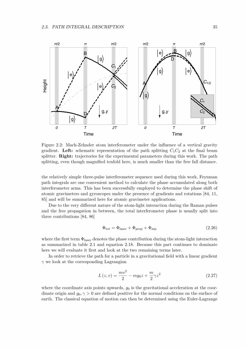
Figure 2.2: Mach-Zehnder atom interferometer under the influence of a vertical gravitygradient. Left: schematic representation of the path splitting C1C2 at the final beamsplitter. Right: trajectories for the experimental parameters during this work. The pathsplitting, even though magnified tenfold here, is much smaller than the free fall distance.
the relatively simple three-pulse interferometer sequence used during this work, Feynmanpath integrals are one convenient method to calculate the phase accumulated along bothinterferometer arms. This has been successfully employed to determine the phase shift ofatomic gravimeters and gyroscopes under the presence of gradients and rotations [84, 11,85] and will be summarized here for atomic gravimeter applications.
Due to the very different nature of the atom-light interaction during the Raman pulsesand the free propagation in between, the total interferometer phase is usually split intothree contributions [84, 86]
Φtot = Φlaser +Φprop +Φsep (2.26)
where the first term Φlaser denotes the phase contribution during the atom-light interactionas summarized in table 2.1 and equation 2.18. Because this part continues to dominatehere we will evaluate it first and look at the two remaining terms later.
In order to retrieve the path for a particle in a gravitational field with a linear gradientγ we look at the corresponding Lagrangian
L (z, v) =mv2
2−mg0z +
m
2γz2 (2.27)
where the coordinate axis points upwards, g0 is the gravitational acceleration at the coor-dinate origin and g0, γ > 0 are defined positive for the normal conditions on the surface ofearth. The classical equation of motion can then be determined using the Euler-Lagrange
36 CHAPTER 2. THEORY
equation which results in hyperbolic trajectories
z(t) =g0γ
+
(z0 −
g0γ
)cosh (
√γt) +
v0 sinh(√
γt)
√γ
(2.28)
≊ −g02t2 + v0t+ z0 + γt2
(− 1
24g0t
2 +1
6v0t+
1
2z0
)(2.29)
The values z0, v0 denote the atomic position and velocity during the first interferometerpulse, e.g. z0 = z(t1). Evaluating the local light phase for the new trajectories againgives ΦLaser as performed previously in equation 2.19, but now also includes the splittingof the paths ABC1 and ADC2. This is executed most easily using computer algebra witha piecewise path definition of the interferometer sequence, where the initial parameters ofeach section are defined by the final position and velocity of the previous section. It yieldsfor upwards directed photon recoil
Φlaser =(ϕA
eff,1 − ϕBeff,2 + ϕC1
eff,3
)−(ϕD
eff,2)
(2.30)
=4keffγ
sinh2
(T√γ
2
)[(z0γ − g0) cosh (T
√γ) + v0
√γ sinh (Tγ)] (2.31)
= keffT2
[g0 + γ
(7
12g0T
2 − v0T − z0
)+O(γ2)
](2.32)
In the limit of vanishing recoil velocity, or infinite atomic mass, this result actually givesthe complete interferometer phase Φtot and will only be corrected bellow to account for thesplitting of the interferometer arms. The measured gravity value in the square brackets isin fact equivalent to measuring the position of a free falling test mass at three points andshows the similarity of this atom interferometer and a classical absolute gravimeter.
In order to obtain the complete interferometer phase including the arm splitting, wenow turn our attention to the last two terms in equation 2.26. Φprop originates from the freepropagation of the wave-packets along both interferometer arms and can be calculated byintegrating the classical action SΓ =
∫Γ L (r(t),v(t)) dt along both arms shown in figure
2.21. Note that in the presence of gradients, the space-time path of both arms don’tgenerally meet at the last pulse. The last term Φsep is associated with the separation ofthe interferometer output ports and closes this gap. We have [84]:
Φprop = (SABC1 − SADC2) /ℏ (2.33)Φsep = p0 · (zC2 − zC1) /ℏ (2.34)
Evaluating Φprop + Φsep with the Lagrangian 2.27 along the exact paths from equation2.28 and summing up with the light phase Φlaser from equation 2.31 yields the totalinterferometer phase shift which, to first order in γ, reads
Φtot = keffT2
[g0 + γ
(7
12g0T
2 −(v0 +
ℏkeff2m
)T − z0
)+O(γ2)
](2.35)
This result is identical to equation 2.31 aside from the replacement v0 → v0 := v0 +ℏkeff2m
which represents the mean path between both interferometer arms depicted as dot-dashed1This approach is formally correct only for Lagrangians up to second order in z,v [84].
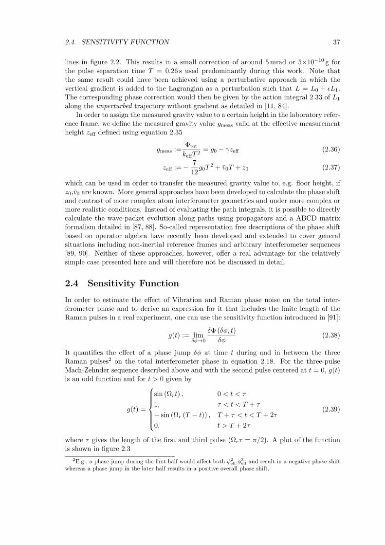
2.4. SENSITIVITY FUNCTION 37
lines in figure 2.2. This results in a small correction of around 5 mrad or 5×10⁻¹⁰ g forthe pulse separation time T = 0.26 s used predominantly during this work. Note thatthe same result could have been achieved using a perturbative approach in which thevertical gradient is added to the Lagrangian as a perturbation such that L = L0 + ϵL1.The corresponding phase correction would then be given by the action integral 2.33 of L1
along the unperturbed trajectory without gradient as detailed in [11, 84].In order to assign the measured gravity value to a certain height in the laboratory refer-
ence frame, we define the measured gravity value gmeas valid at the effective measurementheight zeff defined using equation 2.35
gmeas :=ΦtotkeffT 2
= g0 − γzeff (2.36)
zeff :=− 7
12g0T
2 + v0T + z0 (2.37)
which can be used in order to transfer the measured gravity value to, e.g. floor height, ifz0,v0 are known. More general approaches have been developed to calculate the phase shiftand contrast of more complex atom interferometer geometries and under more complex ormore realistic conditions. Instead of evaluating the path integrals, it is possible to directlycalculate the wave-packet evolution along paths using propagators and a ABCD matrixformalism detailed in [87, 88]. So-called representation free descriptions of the phase shiftbased on operator algebra have recently been developed and extended to cover generalsituations including non-inertial reference frames and arbitrary interferometer sequences[89, 90]. Neither of these approaches, however, offer a real advantage for the relativelysimple case presented here and will therefore not be discussed in detail.
2.4 Sensitivity FunctionIn order to estimate the effect of Vibration and Raman phase noise on the total inter-ferometer phase and to derive an expression for it that includes the finite length of theRaman pulses in a real experiment, one can use the sensitivity function introduced in [91]:
g(t) := limδϕ→0
δΦ(δϕ, t)
δϕ(2.38)
It quantifies the effect of a phase jump δϕ at time t during and in between the threeRaman pulses2 on the total interferometer phase in equation 2.18. For the three-pulseMach-Zehnder sequence described above and with the second pulse centered at t = 0, g(t)is an odd function and for t > 0 given by
g(t) =
sin (Ωrt) , 0 < t < τ
1, τ < t < T + τ
− sin (Ωr (T − t)) , T + τ < t < T + 2τ
0, t > T + 2τ
(2.39)
where τ gives the length of the first and third pulse (Ωrτ = π/2). A plot of the functionis shown in figure 2.3
2E.g., a phase jump during the first half would affect both ϕ2eff,ϕ3
eff and result in a negative phase shiftwhereas a phase jump in the later half results in a positive overall phase shift.

38 CHAPTER 2. THEORY
-
-(+)
-(+)
- (+) (+)
-Figure 2.3: Sensitivity function g(t) of a Mach-Zehnder atom interferometer sequencecentered around t = 0 as defined in equation 2.39.
2.4.1 Finite Raman Pulse Duration
One can now deduce the total interferometer phase by integrating the Raman phase vari-ations ∂tφ over the entire interferometer sequence
∆Φ =
∫ (T+2τ)
−(T+2τ)g(t)
dφ(t)
dtdt (2.40)
When combining this with the local Raman phase from equation 2.19 one obtains a cor-rected form of equation 2.20 that accounts for the finite length of the Raman pulses [74]
∆Φ = (α− keff · g) (T + 2τ)
(T +
4τ
π
)(2.41)
This was confirmed experimentally using GAIN and yielded excellent agreement withinthe measurement resolution of better than 10−9 g. Note that the interferometer phase inequation 2.41 does not scale proportionally to the space-time area enclosed by the Mach-Zehnder sequence anymore, which is proportional to (T + 2τ)T . See [92] for an extendedformalism and detailed description of this topic.
For the practical application as atomic gravimeter, however, this is of little interest asthe atom interferometer is usually operated on the central, or dark, fringe around ∆Φ ≈ 0which is insensitive to this scaling. The next chapter will therefore turn to the estimationof phase noise using the sensitivity function.
2.4.2 Raman Laser Phase Noise
The sensitivity function can also be used to estimate the effect of Raman phase noise onthe interferometer phase. The transfer function from phase noise of the Raman laser tothe interferometer output is derived from the sensitivity function Fourier transform G(ω)
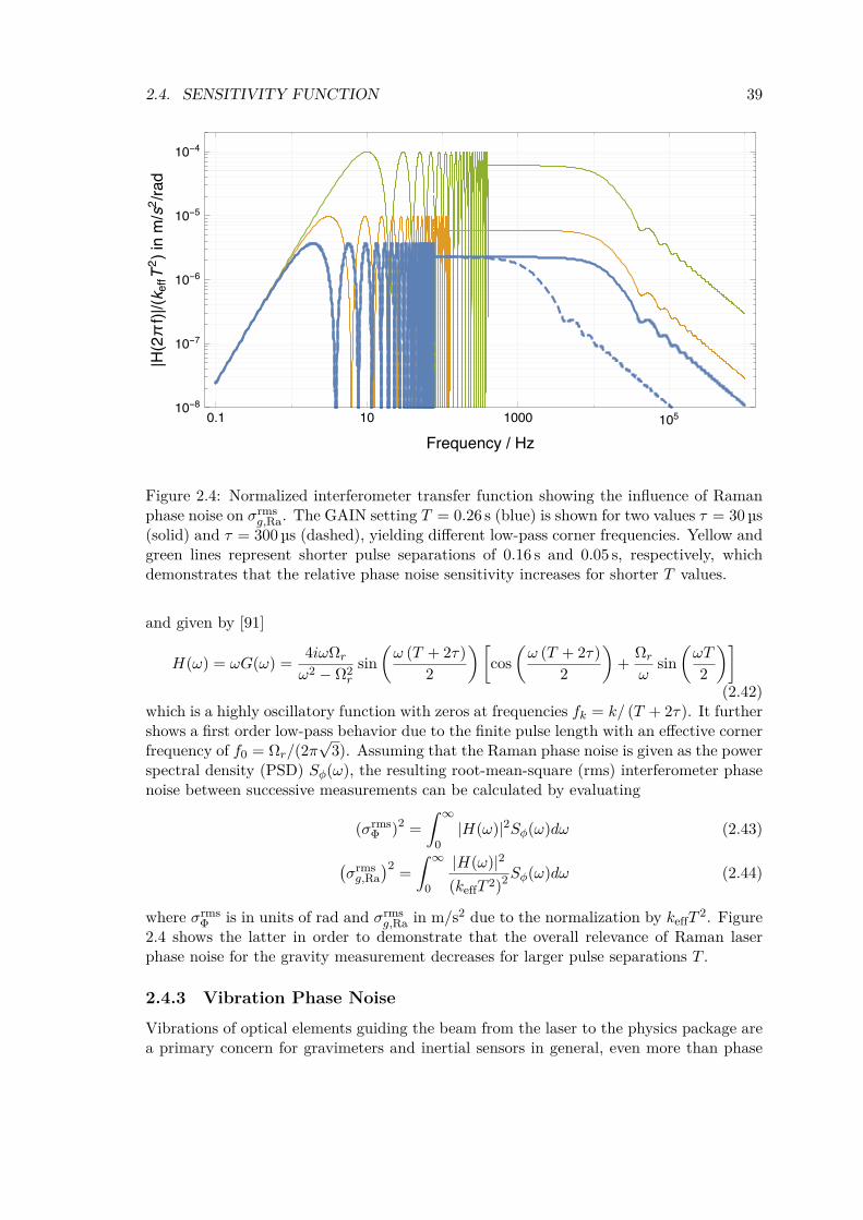
2.4. SENSITIVITY FUNCTION 39
-
-
-
-
-
/
|()|/(
)//
Figure 2.4: Normalized interferometer transfer function showing the influence of Ramanphase noise on σrms
g,Ra. The GAIN setting T = 0.26 s (blue) is shown for two values τ = 30 µs(solid) and τ = 300 µs (dashed), yielding different low-pass corner frequencies. Yellow andgreen lines represent shorter pulse separations of 0.16 s and 0.05 s, respectively, whichdemonstrates that the relative phase noise sensitivity increases for shorter T values.
and given by [91]
H(ω) = ωG(ω) =4iωΩr
ω2 − Ω2r
sin(ω (T + 2τ)
2
)[cos
(ω (T + 2τ)
2
)+
Ωr
ωsin
(ωT
2
)](2.42)
which is a highly oscillatory function with zeros at frequencies fk = k/ (T + 2τ). It furthershows a first order low-pass behavior due to the finite pulse length with an effective cornerfrequency of f0 = Ωr/(2π
√3). Assuming that the Raman phase noise is given as the power
spectral density (PSD) Sφ(ω), the resulting root-mean-square (rms) interferometer phasenoise between successive measurements can be calculated by evaluating
(σrmsΦ )2 =
∫ ∞
0|H(ω)|2Sφ(ω)dω (2.43)
(σrmsg,Ra
)2=
∫ ∞
0
|H(ω)|2
(keffT 2)2Sφ(ω)dω (2.44)
where σrmsΦ is in units of rad and σrms
g,Ra in m/s2 due to the normalization by keffT2. Figure
2.4 shows the latter in order to demonstrate that the overall relevance of Raman laserphase noise for the gravity measurement decreases for larger pulse separations T .
2.4.3 Vibration Phase NoiseVibrations of optical elements guiding the beam from the laser to the physics package area primary concern for gravimeters and inertial sensors in general, even more than phase
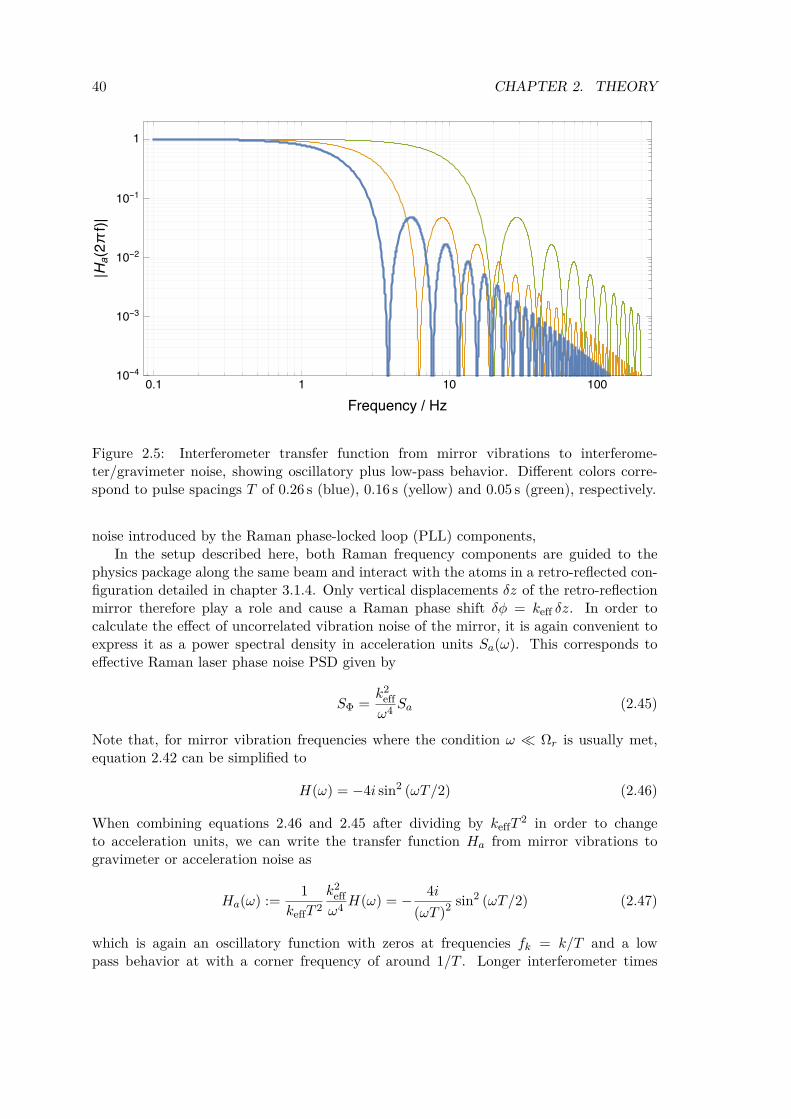
40 CHAPTER 2. THEORY
-
-
-
-
/
|()|
Figure 2.5: Interferometer transfer function from mirror vibrations to interferome-ter/gravimeter noise, showing oscillatory plus low-pass behavior. Different colors corre-spond to pulse spacings T of 0.26 s (blue), 0.16 s (yellow) and 0.05 s (green), respectively.
noise introduced by the Raman phase-locked loop (PLL) components,In the setup described here, both Raman frequency components are guided to the
physics package along the same beam and interact with the atoms in a retro-reflected con-figuration detailed in chapter 3.1.4. Only vertical displacements δz of the retro-reflectionmirror therefore play a role and cause a Raman phase shift δφ = keff δz. In order tocalculate the effect of uncorrelated vibration noise of the mirror, it is again convenient toexpress it as a power spectral density in acceleration units Sa(ω). This corresponds toeffective Raman laser phase noise PSD given by
SΦ =k2effω4
Sa (2.45)
Note that, for mirror vibration frequencies where the condition ω Ωr is usually met,equation 2.42 can be simplified to
H(ω) = −4i sin2 (ωT/2) (2.46)
When combining equations 2.46 and 2.45 after dividing by keffT2 in order to change
to acceleration units, we can write the transfer function Ha from mirror vibrations togravimeter or acceleration noise as
Ha(ω) :=1
keffT 2
k2effω4
H(ω) = − 4i
(ωT )2sin2 (ωT/2) (2.47)
which is again an oscillatory function with zeros at frequencies fk = k/T and a lowpass behavior at with a corner frequency of around 1/T . Longer interferometer times

2.4. SENSITIVITY FUNCTION 41
T therefore reduce the sensitivity to higher frequency vibrations. Note, however, thatfor larger T the absolute phase noise increases quadratically so that the vibration noiseexpressed in rad grows rapidly. Without countermeasures such as a vibration isolationsystem, this quickly leads to washed out interference fringes and loss of phase information.These properties of equation 2.47 were the main driving forces for the design of the activevibration isolator described in chapter 3.2.
Analogous to equation 2.44, Ha(ω) can be used to estimate the rms noise of successiveinterferometer measurements caused by parasitic mirror vibrations. If the spectral densityof the mirror vibrations is measured by an appropriate sensor as described in chapter 3.2it can be readily calculated with
(σrmsg,vib
)2=
∫ ∞
0|Ha(ω)|2Sa(ω)dω (2.48)
Moreover, the sensitivity function 2.38 can be used directly in this case in order to derivethe vibration induced phase as detailed in chapter 3.2.2.
SummaryThis chapter gave a brief introduction of the atom-light interaction during stimulatedRaman transitions and derived the atom interferometer phase with path integrals includingall necessary corrections to measure the local gravity value with an accuracy of betterthan 10−9 g. Furthermore, the sensitivity function as a general tool to describe the totalinterferometer phase and the influence of the most important noise sources was introduced.Chapter 3 will now give a detailed account of the transportable experimental apparatusthat was used for the gravity measurements presented later on in this thesis.

42 CHAPTER 2. THEORY
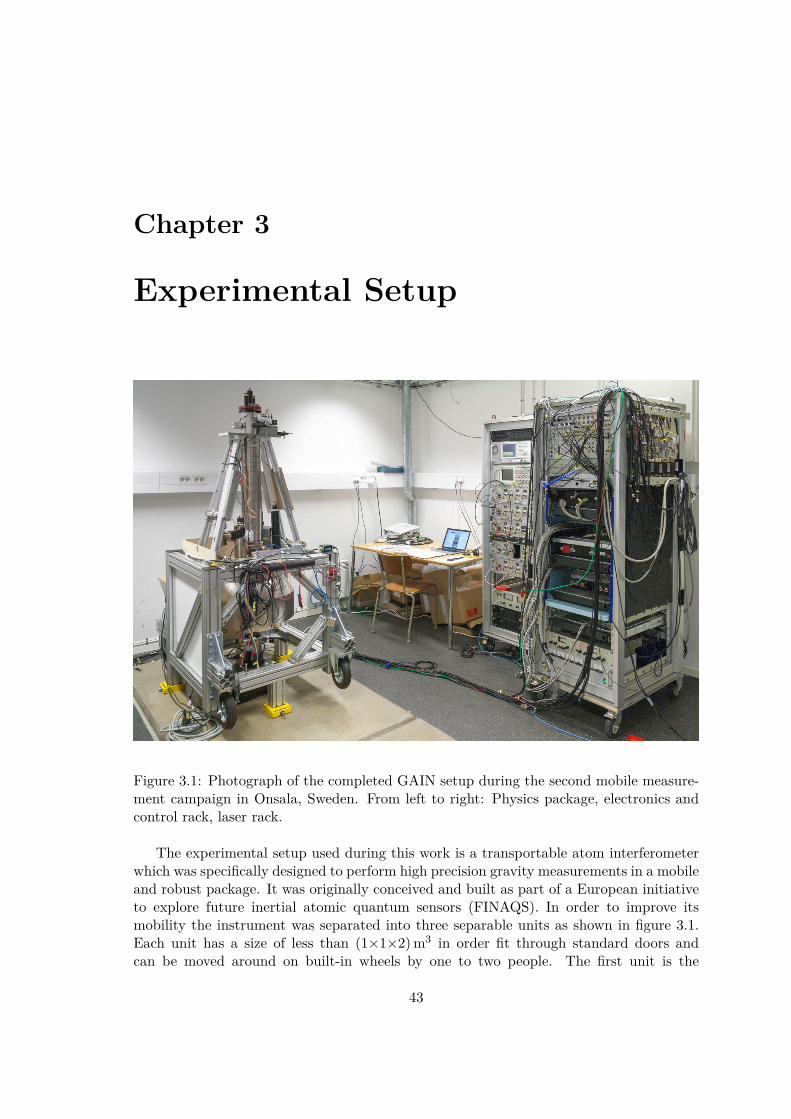
Chapter 3
Experimental Setup
Figure 3.1: Photograph of the completed GAIN setup during the second mobile measure-ment campaign in Onsala, Sweden. From left to right: Physics package, electronics andcontrol rack, laser rack.
The experimental setup used during this work is a transportable atom interferometerwhich was specifically designed to perform high precision gravity measurements in a mobileand robust package. It was originally conceived and built as part of a European initiativeto explore future inertial atomic quantum sensors (FINAQS). In order to improve itsmobility the instrument was separated into three separable units as shown in figure 3.1.Each unit has a size of less than (1×1×2)m3 in order fit through standard doors andcan be moved around on built-in wheels by one to two people. The first unit is the
43

44 CHAPTER 3. EXPERIMENTAL SETUP
physics package containing the vacuum system were the actual gravity measurement takesplace. A 19” rack containing the laser system forms the second unit which delivers allnecessary optical frequencies to the physics package through optical fibers. All systemsare powered and controlled from the third unit which is another 19” rack also containingtwo computers for sequence control and data storage, respectively. The first version of theinstrument was completed and described in earlier works [82, 93, 94], and the first gravitymeasurements were conducted at Humboldt Universität zu Berlin in 2010. In order toreach the original goal of performing gravity measurements on remote sites beyond thestate-of-the-art, several improvements of the existing hardware and additional subsystemshad to be implemented as part of this work, such as a Tip/Tilt mirror or a magnetic shieldaround the MOT-chamber. This chapter includes a short, but comprehensive descriptionof the overall experimental apparatus with references to previous results, as well as adetailed analysis of subsystems that were added or modified as part of this work.
3.1 Physics PackageThe experimental apparatus is built around an atomic fountain with an elongated inter-ferometry section and vertical Raman beams retro-reflected by a mirror below the vacuumsystem. This well-known retro-reflection architecture has the advantage that phase-noiseof the Raman beams due to vibrations of all optical elements are common mode and cancelout in the gravity measurement, with the exception of the retro-reflection mirror whichprovides the inertial reference. The fountain chamber was designed for uncompromisinggravimeter performance using a relatively long, magnetically shielded interferometer zone,but also with flexibility in mind providing a total of 42 view ports. The physics packagecan be divided into four functional parts as shown in figure 3.2. The first part is theelongated interferometer zone on top, the second the state selection and detection zonein the middle and third the MOT region in the bottom of the vacuum system which pro-vides the pulsed source of laser-cooled Rubidium. Finally, the Raman retro-reflector onthe vibration isolation system below the vacuum system. A schematic overview of thesefunctional elements is depicted in figure 3.2 and each part will be reviewed in the followingsub-chapters.
3.1.1 Vacuum SystemThe main part of the physics package is the elongated, roughly 1.15 m tall atomic fountainUHV chamber shown in figure 3.2. The UHV environment is necessary to prevent atomlosses during the course of a measurement due to interactions with the background gas.Most parts of the vacuum system are milled from solid blocks of Titanium alloy due to itsadvantageous mechanical and vacuum properties. Its low specific conductivity furthermoreenables faster decay of eddy currents than in an equivalent welded steel chamber. Conflat(CF) flanges and Indium sealed windows keep the integrated leak rate small enough toreach a base pressure of a few 10−10 hPa despite the large number of windows. A 20 l/sion pump and a Titanium sublimation pump attached to the detection region maintainthese conditions (not shown in figure 3.2). See [93] for a more detailed description of thevacuum system.
The Rubidium source for the fountain was originally provided by dispensers fromSAES getters [93]. Unfortunately, they were completely depleted during the middle of this
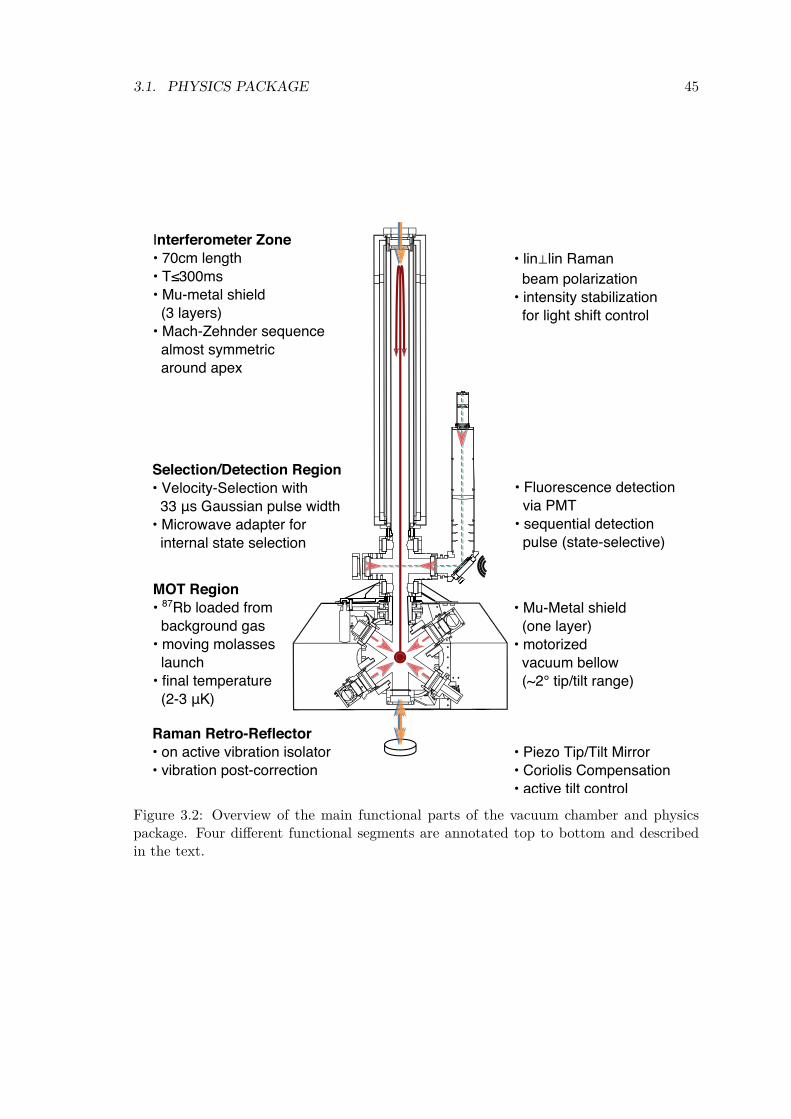
3.1. PHYSICS PACKAGE 45
• Fluorescence detection via PMT• sequential detection pulse (state-selective)
Interferometer Zone• 70cm length • T 300ms• Mu-metal shield (3 layers)• Mach-Zehnder sequence almost symmetric around apex
Raman Retro-Reflector• on active vibration isolator• vibration post-correction
• lin lin Raman beam polarization• intensity stabilization for light shift control
MOT Region• 87Rb loaded from background gas• moving molasses launch• final temperature (2-3 K)
• Mu-Metal shield (one layer)• motorized vacuum bellow (~2° tip/tilt range)
Selection/Detection Region• Velocity-Selection with 33 s Gaussian pulse width• Microwave adapter for internal state selection
• Piezo Tip/Tilt Mirror• Coriolis Compensation• active tilt control
Figure 3.2: Overview of the main functional parts of the vacuum chamber and physicspackage. Four different functional segments are annotated top to bottom and describedin the text.
46 CHAPTER 3. EXPERIMENTAL SETUP
work and had to be replaced in order to conduct the second mobile gravity measurementsuccessfully. The new dispensers by the company Alvatec and have a strongly increasedcapacity1 compared to the previously used models. They emit Rubidium in its naturalisotopic abundances and feature significantly reduced emission of spurious elements duringoperation. This reduced the vacuum pressure during fountain operation by nearly oneorder of magnitude with respect to the previous sources to a few times 10−10 hPa whilestill providing sufficient Rb to load the MOT within 0.6 s.
A replacement of the dispenser assembly without breaking the vacuum had been an-ticipated during the construction of the vacuum chamber which is why it was separatedusing a UHV gate valve2. Unfortunately, the valve‘s Viton seal had been damaged which,according to the manufacturer, was most likely caused by accelerated aging under theconstant exposure to chemically reactive Rubidium. Performing this switching operationwithout compromising the UHV conditions in the main chamber therefore turned out tobe challenging. By working in a glove-bag filled with dry nitrogen atmosphere evaporatedfrom a LN2 dewar, a renewed bake-out could nevertheless be avoided.
3.1.2 MOT Chamber
The bottom section of the chamber contains a MOT which prepares the laser-cooled atomsfor the fountain [81]. Six circularly polarized laser beams with a diameter of 30 mm (1/e2)in a 1-1-1 configuration intersect at the MOT center. In this arrangement every beamencloses an angle of 54.7 ° to the vertical. A magnetic quadrupole field is generated by twoair-cooled anti-Helmholtz coils which results in a central field gradient of approximately0.5 mT/cm [93] at a current of 8 A. The 87Rb atoms are released into the chamber throughresistive heating of the Rubidium dispensers and loaded into the MOT from backgroundgas. The Rb pressure in the vacuum system can be finely controlled through variationsof the dispenser heating current, which is applied continuously during fountain operation.The MOT chamber furthermore provides a tip/tilt mechanism through a vacuum bellowwhich is essential for fine-tuning of the launch direction as described in [93]. In order tocompensate for background magnetic fields, bias coils were implemented and fine-tunedin order to achieve the required µK temperatures during the moving molasses launch.In order to monitor the size and shape of the MOT during loading and launch, threetriggered CMOS cameras are attached to the MOT chamber at different angles. The finalatom number in the MOT before launch can be estimated from fluorescence captured bythe cameras to around 109 87Rb atoms.
Magnetic Shield Implementation
During this work a magnetic shield was designed and implemented around the MOT-Chamber. It serves the two interrelated purposes of shielding the MOT from backgroundmagnetic fields and isolating the rest of the set-up from switching fields generated bythe MOT-coils, which turned out to have a particularly detrimental effect on gravityobservations through the vibration isolator right underneath the MOT chamber as detailedin chapter 6.5.1. Due to the comparatively small dimensions of the GAIN MOT chamber,two issues had to be overcome while designing the magnetic shield. First, the shield had to
14 dispensers containing 35 mg of Rubidium each2VAT Mini UHV gate valve, Series 010
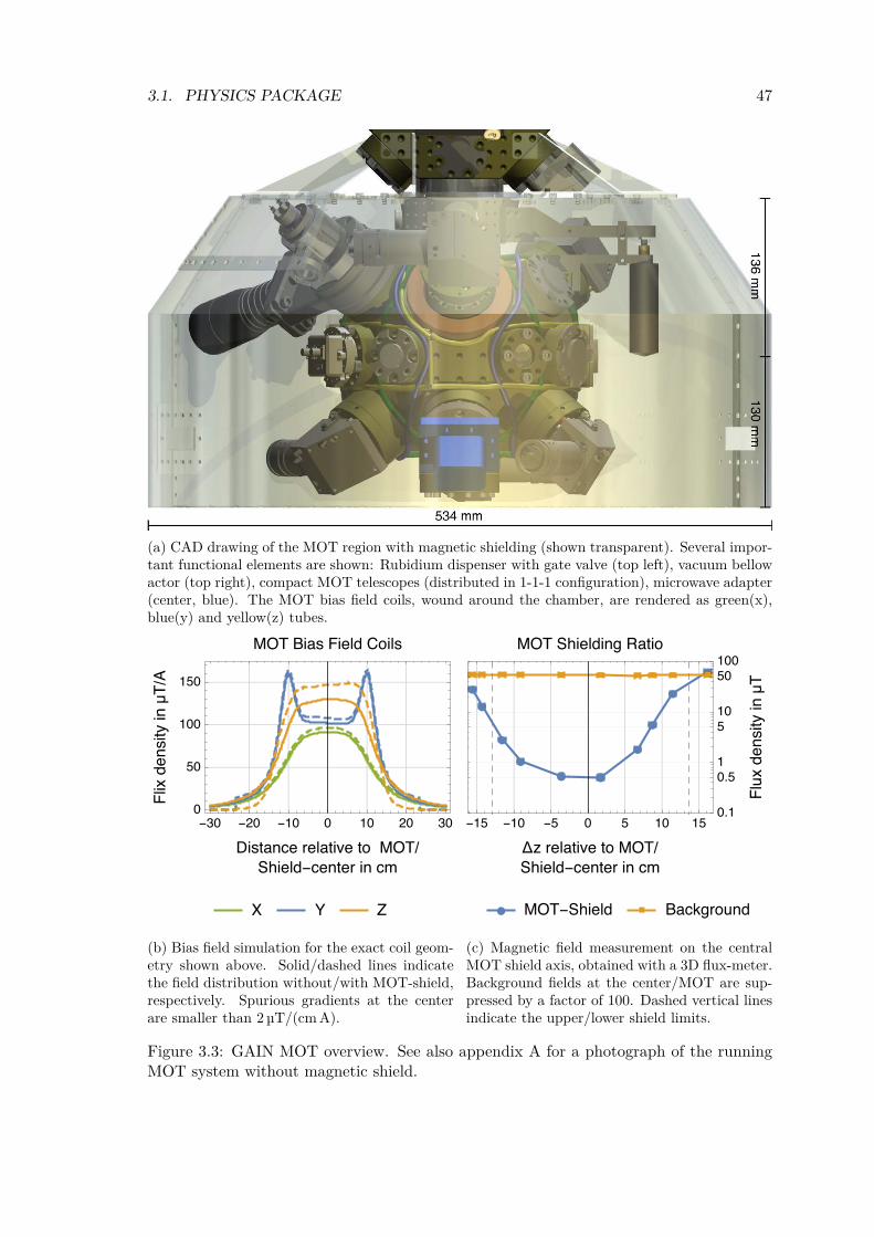
3.1. PHYSICS PACKAGE 47
(a) CAD drawing of the MOT region with magnetic shielding (shown transparent). Several impor-tant functional elements are shown: Rubidium dispenser with gate valve (top left), vacuum bellowactor (top right), compact MOT telescopes (distributed in 1-1-1 configuration), microwave adapter(center, blue). The MOT bias field coils, wound around the chamber, are rendered as green(x),blue(y) and yellow(z) tubes.
- - - /-
µ/
(b) Bias field simulation for the exact coil geom-etry shown above. Solid/dashed lines indicatethe field distribution without/with MOT-shield,respectively. Spurious gradients at the centerare smaller than 2 µT/(cm A).
- - - /-
µ
-(c) Magnetic field measurement on the centralMOT shield axis, obtained with a 3D flux-meter.Background fields at the center/MOT are sup-pressed by a factor of 100. Dashed vertical linesindicate the upper/lower shield limits.
Figure 3.3: GAIN MOT overview. See also appendix A for a photograph of the runningMOT system without magnetic shield.
48 CHAPTER 3. EXPERIMENTAL SETUP
be engineered tightly around the compact vacuum joint in order to provide good shieldingcharacteristics at the MOT position without constraining the vacuum bellow. Second, theprevious bias field coils used until then were far too bulky to fit into the shield and hadto be redesigned completely.
The first issue was addressed with a cylindric one-layered Mu-Metal shield carefullydesigned to fit around the MOT section of the vacuum chamber with minimal opening atboth top and bottom for the vacuum bellow and Raman beam, respectively. It is shownin the bottom of figures 3.1 and 3.2 and detailed in the CAD drawing in figure 3.3. Inorder to enable quick access to the MOT chamber it consists of two removable segments.One extension port close to the dispenser assembly enables future additions to the MOTchamber, such as a 2D-MOT, in order to enable faster MOT loading [95, 96]. The vacuumjoint actors were furthermore adapted to allow remote motorized tip/tilt operation, whichwas necessary as the magnetic shield otherwise prevents access.
In order to provide a homogeneous bias field at the location of the MOT without theneed for bulky Helmholtz coil pairs, the respective coils were wound directly around theMOT chamber. A preceding FEM simulation of the resulting field was used to find aconfiguration with 4 coils for each axis that delivers reasonable homogeneity of the biasfield despite the otherwise unsuitable geometry of the MOT chamber. See figure 3.3 for aCAD drawing of the final MOT setup and the simulated magnetic field distribution.
The measured shielding behavior displayed in figure 3.3c shows a reduction of back-ground fields of around two orders of magnitude at the location of the MOT, which agreeswell with FEM simulation. This enables mG background fields without active compen-sation and almost supersedes the need for a homogeneous bias field altogether. This isconfirmed by the atomic fountain optimization where the bias coils are now only used toseparate the magnetic sub-levels during velocity selection.
3.1.3 Detection and State-Selection Chamber
The central section of the vacuum chamber consists of an octagonally shaped region, whichprovides twelve access ports on three horizontal(x-y) planes and four diagonal view-portson vertical(x-z) plane. See figure 3.4 for cut-view schematics of the overall geometry. Bothvacuum pumps are mounted along a horizontal axis in close proximity to the detectionarea. This minimizes the background gas pressure compared to other parts of the chamberwhich benefits the signal to background ratio during detection. To facilitate the state-selection a microwave adapter is mounted along the pumping axis which, compared to aprevious configuration perpendicular to this axis, frees up one more axis for optical access.Light from an auxiliary fiber coupled to both repump- and cooling-laser enter the chamberthrough a diagonal view-port to implement resonant blow-away pulses for both hyperfineground states. Three additional diagonal view-ports are available and could be used, e.g.,for the implementation of advanced detection schemes or cooling methods such as Ramansideband cooling.
The fluorescence detection system consists of a resonant collimated beam which isretro-reflected in the central detection zone. The beam has a diameter of around 50 mm(1/e2) and can be stopped down using a diaphragm aperture to a diameter Ddet that canbe varied between 5–30 mm. Both F = 1 and F = 2 resonant light can be coupled into thisbeam through independent AOMs, which allows to facilitate the state-selective detectionsequence. The fluorescence light of the atoms in the detection area is imaged onto the

3.1. PHYSICS PACKAGE 49
C
C
UHV
Gauge
Microwave
Adapter
Detection
beam
Mirror
PMT
Ion P
ump
Ti-Sub
Pump y
x
Blow-awaybeams
atoms
x
z
PMT
Mirror
C-C
vdet
toInterferom
eterZone
toMOTDdet
Figure 3.4: State-selection and detection region in simplified horizontal(left) and verti-cal(right) cut-views. The fluorescence detection system, blow-away beams and microwaveadapter for state-selection and vacuum pumps are depicted schematically. Free diagonalview-ports for future modification are indicated on the vertical cut-view.
PMT by two plano-convex lenses3 in a scale-preserving 1f-1f configuration, collecting asolid angle of around 4π × 0.017 sr. An aperture with 4 mm horizontal width in front ofthe PMT restricts the size of the detection region and minimizes stray light in combinationwith a conically-shaped beam-dump behind the opposite view-port. In order to measurethe relative population of both hyperfine states, a state-selective detection sequence isused which will be detailed in chapter 4.4.
3.1.4 Interferometer Zone and Raman Beams
The section in which the atom interferometry takes place consists of a magneticallyshielded, cylindrical region with a length of 0.7 m as indicated in figure 3.2. Both Ramanbeam frequency components enter the chamber from above through the same telescopewith a beam diameter of 30 mm (1/e2) in the same linear polarization. They are thenretro-reflected through a quarter wave-plate in the orthogonal linear polarization on theway back to the Raman telescope (lin⊥lin configuration). Since the quantization axisprovided by the vertical magnetic bias field is parallel to the Raman wave-vector keff, thisconfiguration only drives σ± transition as indicated in figure 3.5. Counter-propagatingbeam pairs then drive Doppler-sensitive σ+σ+ and σ−σ− transitions with ∆m = 0 in
3PMT R10699, Hamamatsu; Lens: clear aperture 38 mm, focal length 70 mm
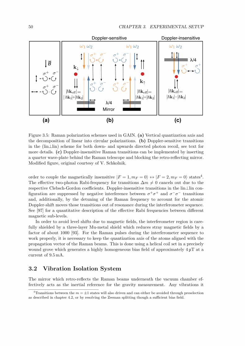
50 CHAPTER 3. EXPERIMENTAL SETUP
B
= ++
= -
(a) (b) (c)
++
-
++
-
Doppler-sensitive Doppler-insensitive
Mirror/4
/4
Figure 3.5: Raman polarization schemes used in GAIN. (a) Vertical quantization axis andthe decomposition of linear into circular polarizations. (b) Doppler-sensitive transitionsin the (lin⊥lin) scheme for both down- and upwards directed photon recoil, see text formore details. (c) Doppler-insensitive Raman transitions can be implemented by insertinga quarter wave-plate behind the Raman telescope and blocking the retro-reflecting mirror.Modified figure, original courtesy of V. Schkolnik.
order to couple the magnetically insensitive |F = 1,mF = 0〉 ↔ |F = 2,mF = 0〉 states4.The effective two-photon Rabi-frequency for transitions ∆m = 0 cancels out due to therespective Clebsch-Gordon coefficients. Doppler-insensitive transitions in the lin⊥lin con-figuration are suppressed by negative interference between σ+σ+ and σ−σ− transitionsand, additionally, by the detuning of the Raman frequency to account for the atomicDoppler-shift moves those transitions out of resonance during the interferometer sequence.See [97] for a quantitative description of the effective Rabi frequencies between differentmagnetic sub-levels.
In order to avoid level shifts due to magnetic fields, the interferometer region is care-fully shielded by a three-layer Mu-metal shield which reduces stray magnetic fields by afactor of about 1000 [93]. For the Raman pulses during the interferometer sequence towork properly, it is necessary to keep the quantization axis of the atoms aligned with thepropagation vector of the Raman beams. This is done using a helical coil set in a preciselywound grove which generates a highly homogeneous bias field of approximately 4 µT at acurrent of 9.5 mA.
3.2 Vibration Isolation SystemThe mirror which retro-reflects the Raman beams underneath the vacuum chamber ef-fectively acts as the inertial reference for the gravity measurement. Any vibrations it
4Transitions between the m = ±1 states will also driven and can either be avoided through preselectionas described in chapter 4.2, or by resolving the Zeeman splitting though a sufficient bias field.

3.2. VIBRATION ISOLATION SYSTEM 51
exhibits during the interferometer therefore enter as phase noise and shift the measuredgravity value. This is especially severe for low frequency vibrations below 1/T ≊ 4 Hz dueto the interferometer transfer function shown in figure 2.5. Moreover, with the compar-atively large pulse spacing T = 0.26 s used here during the gravity measurements, thisphase noise easily has an amplitude of several radian which makes it difficult to assign aspecific data point to the correct interferometer fringe and extract the phase information.Two established approaches exist in order to deal with this problem: isolating the mirrorfrom external vibrations very carefully using specialized active isolation systems [98], orrecording the vibrations and removing their effect using a post-correction algorithm [99].The lowest vibration induced phase noise published [12] so far was found using the firstapproach whereas the second method is very attractive for mobile instruments due to thesimple and compact architecture. In this work both strategies were combined by activelyisolating the mirror and additionally removing remaining vibration in the feedback errorsignal in post-correction.
3.2.1 Active Vibration IsolatorA customized active vibration isolator was developed, built and characterized during anearlier work of the author [94, 93]. It was improved as part of this thesis by locating andcentering the accelerometer axis exactly below the mirror and platform center in orderto minimize cross-coupling of horizontal vibrations. Additionally, the control softwarewas extended to allow for more general feedback filter parameters and sub-ms level syn-chronization with the interferometer sequence which is important for post-correction. ATip/Tilt system for the retro-reflecting mirror was also implemented to allow for compen-sation of the Coriolis effect and is described in chapter 3.2.3. The rest of this chapterwill briefly introduce the active system with special emphasis on the implemented im-provements. For a more detailed description of the mechanical system and feedback loopparameters, refer to [94]. An illustration of the system can be found in figure 3.6. Itis based on a commercial passive vibration isolation platform Minusk 50BM-10 with aneffective resonance frequency of 0.5 Hz along vertical and horizontal5 direction. In orderto minimize the non-linearity of the negative-stiffness mechanism, the passive vertical res-onance frequency is actually tuned slightly higher to 0.7 Hz, see [94]. Residual vibrationson the platform are measured by a low-noise seismometer Guralp CMG-3VL with a band-width of 0.005–100 Hz. The acceleration signal is fed into a digital feedback filter basedon a NI compactRIO real-time system. A field-programmable gate array (FPGA) with a24 bit analog-to-digital converter (ADC) and a 16 bit digital-to-analog converter (DAC)implements the digital filter with a sample rate of 1562.5 Hz, which is around two orders ofmagnitude higher than the achieved control bandwidth. The filtered voltage signal is thenfed into a voltage-controlled current source. It sends a current to two voice-coil actuatorswhich are built into the vertical isolation stage of the MinusK platform and exert a forcebetween its top and bottom in order to close the feedback loop. Special care was takento make sure that no mechanical friction is introduced by the voice coils which wouldotherwise drastically reduce the effectiveness of the passive isolation system.
The behavior of the active system under quiet and noisy environmental conditions isdepicted in figure 3.7 which shows amplitude spectral densities, absolute transmissibility
5Custom-built columns from MinusK and improved leveling feet were used to achieve the 0.5 Hz hori-zontal resonance frequency of the inverted pendulum mechanism as described in [94]
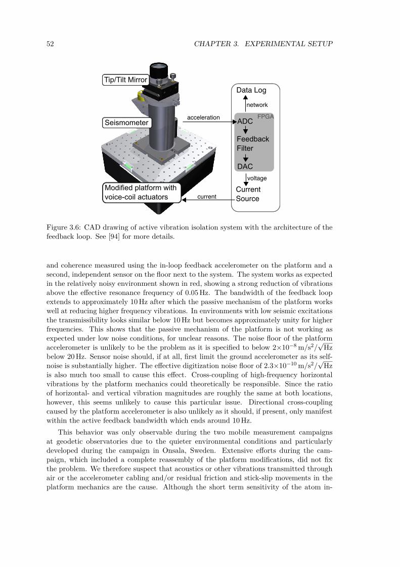
52 CHAPTER 3. EXPERIMENTAL SETUP
Seismometer
Tip/Tilt Mirror
Modified platform withvoice-coil actuators
acceleration
currentCurrentSource
Data Log
ADC
FeedbackFilter
DAC
FPGAnetwork
voltage
Figure 3.6: CAD drawing of active vibration isolation system with the architecture of thefeedback loop. See [94] for more details.
and coherence measured using the in-loop feedback accelerometer on the platform and asecond, independent sensor on the floor next to the system. The system works as expectedin the relatively noisy environment shown in red, showing a strong reduction of vibrationsabove the effective resonance frequency of 0.05 Hz. The bandwidth of the feedback loopextends to approximately 10 Hz after which the passive mechanism of the platform workswell at reducing higher frequency vibrations. In environments with low seismic excitationsthe transmissibility looks similar below 10 Hz but becomes approximately unity for higherfrequencies. This shows that the passive mechanism of the platform is not working asexpected under low noise conditions, for unclear reasons. The noise floor of the platformaccelerometer is unlikely to be the problem as it is specified to below 2×10⁻⁸ m/s2/
√Hz
below 20 Hz. Sensor noise should, if at all, first limit the ground accelerometer as its self-noise is substantially higher. The effective digitization noise floor of 2.3×10⁻¹⁰ m/s2/
√Hz
is also much too small to cause this effect. Cross-coupling of high-frequency horizontalvibrations by the platform mechanics could theoretically be responsible. Since the ratioof horizontal- and vertical vibration magnitudes are roughly the same at both locations,however, this seems unlikely to cause this particular issue. Directional cross-couplingcaused by the platform accelerometer is also unlikely as it should, if present, only manifestwithin the active feedback bandwidth which ends around 10 Hz.
This behavior was only observable during the two mobile measurement campaignsat geodetic observatories due to the quieter environmental conditions and particularlydeveloped during the campaign in Onsala, Sweden. Extensive efforts during the cam-paign, which included a complete reassembly of the platform modifications, did not fixthe problem. We therefore suspect that acoustics or other vibrations transmitted throughair or the accelerometer cabling and/or residual friction and stick-slip movements in theplatform mechanics are the cause. Although the short term sensitivity of the atom in-
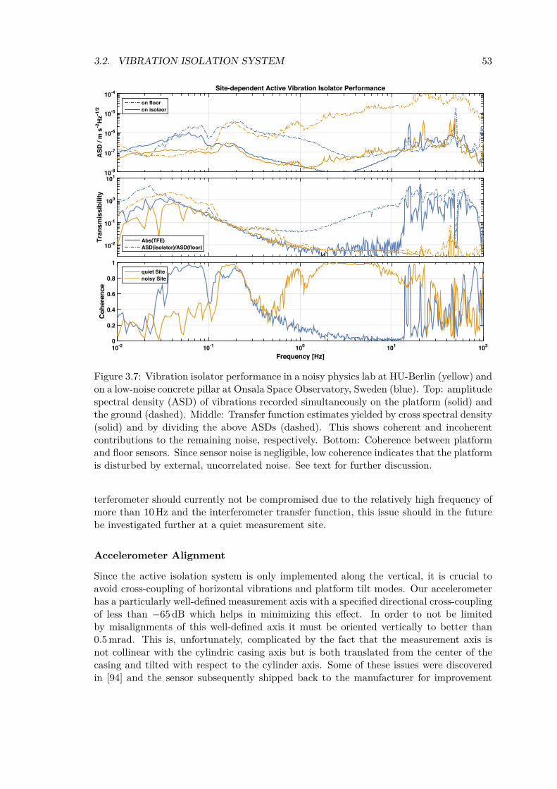
3.2. VIBRATION ISOLATION SYSTEM 53
ASD
/ m
s-2
Hz-1
/2
10-8
10-7
10-6
10-5
10-4Site-dependent Active Vibration Isolator Performance
on flooron isolaor
Tran
smis
sibi
lity
10-2
10-1
100
101
Abs(TFE)ASD(isolator)/ASD(floor)
Frequency [Hz]10-2 10-1 100 101 102
Coh
eren
ce
0
0.2
0.4
0.6
0.8
1quiet Sitenoisy Site
Figure 3.7: Vibration isolator performance in a noisy physics lab at HU-Berlin (yellow) andon a low-noise concrete pillar at Onsala Space Observatory, Sweden (blue). Top: amplitudespectral density (ASD) of vibrations recorded simultaneously on the platform (solid) andthe ground (dashed). Middle: Transfer function estimates yielded by cross spectral density(solid) and by dividing the above ASDs (dashed). This shows coherent and incoherentcontributions to the remaining noise, respectively. Bottom: Coherence between platformand floor sensors. Since sensor noise is negligible, low coherence indicates that the platformis disturbed by external, uncorrelated noise. See text for further discussion.
terferometer should currently not be compromised due to the relatively high frequency ofmore than 10 Hz and the interferometer transfer function, this issue should in the futurebe investigated further at a quiet measurement site.
Accelerometer Alignment
Since the active isolation system is only implemented along the vertical, it is crucial toavoid cross-coupling of horizontal vibrations and platform tilt modes. Our accelerometerhas a particularly well-defined measurement axis with a specified directional cross-couplingof less than −65 dB which helps in minimizing this effect. In order to not be limitedby misalignments of this well-defined axis it must be oriented vertically to better than0.5 mrad. This is, unfortunately, complicated by the fact that the measurement axis isnot collinear with the cylindric casing axis but is both translated from the center of thecasing and tilted with respect to the cylinder axis. Some of these issues were discoveredin [94] and the sensor subsequently shipped back to the manufacturer for improvement
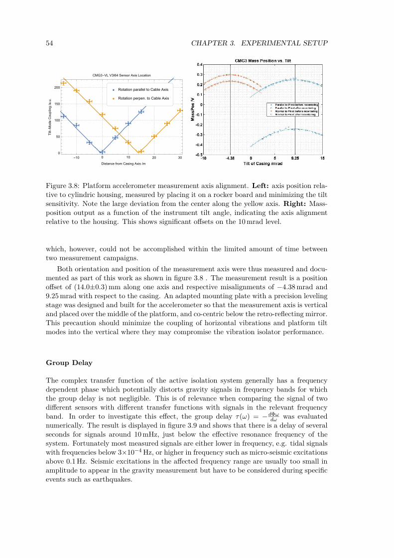
54 CHAPTER 3. EXPERIMENTAL SETUP
Rotation parallel to Cable Axis
Rotation to Cable Axis
-10 20 300
50
100
150
200
0 10
Distance from Axis /m
Tilt-Mo
deCoupling/a.u.
CMG3-VL V3I64 Sensor Axis Location
Figure 3.8: Platform accelerometer measurement axis alignment. Left: axis position rela-tive to cylindric housing, measured by placing it on a rocker board and minimizing the tiltsensitivity. Note the large deviation from the center along the yellow axis. Right: Mass-position output as a function of the instrument tilt angle, indicating the axis alignmentrelative to the housing. This shows significant offsets on the 10 mrad level.
which, however, could not be accomplished within the limited amount of time betweentwo measurement campaigns.
Both orientation and position of the measurement axis were thus measured and docu-mented as part of this work as shown in figure 3.8 . The measurement result is a positionoffset of (14.0±0.3)mm along one axis and respective misalignments of −4.38 mrad and9.25 mrad with respect to the casing. An adapted mounting plate with a precision levelingstage was designed and built for the accelerometer so that the measurement axis is verticaland placed over the middle of the platform, and co-centric below the retro-reflecting mirror.This precaution should minimize the coupling of horizontal vibrations and platform tiltmodes into the vertical where they may compromise the vibration isolator performance.
Group Delay
The complex transfer function of the active isolation system generally has a frequencydependent phase which potentially distorts gravity signals in frequency bands for whichthe group delay is not negligible. This is of relevance when comparing the signal of twodifferent sensors with different transfer functions with signals in the relevant frequencyband. In order to investigate this effect, the group delay τ(ω) = −dΦω
dω was evaluatednumerically. The result is displayed in figure 3.9 and shows that there is a delay of severalseconds for signals around 10 mHz, just below the effective resonance frequency of thesystem. Fortunately most measured signals are either lower in frequency, e.g. tidal signalswith frequencies below 3×10⁻⁴ Hz, or higher in frequency such as micro-seismic excitationsabove 0.1 Hz. Seismic excitations in the affected frequency range are usually too small inamplitude to appear in the gravity measurement but have to be considered during specificevents such as earthquakes.
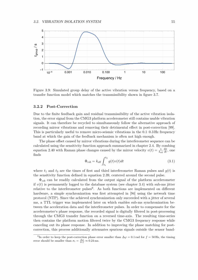
3.2. VIBRATION ISOLATION SYSTEM 55
--/
/
Figure 3.9: Simulated group delay of the active vibration versus frequency, based on atransfer function model which matches the transmissibility shown in figure 3.7.
3.2.2 Post-Correction
Due to the finite feedback gain and residual transmissibility of the active vibration isola-tion, the error signal from the CMG3 platform accelerometer still contains usable vibrationsignals. It can therefore be recycled to simultaneously follow the alternative approach ofrecording mirror vibrations and removing their detrimental effect in post-correction [99].This is particularly useful to remove micro-seismic vibrations in the 0.1–0.3 Hz frequencyband at which the gain of the feedback mechanism is often not high enough.
The phase offset caused by mirror vibrations during the interferometer sequence can becalculated using the sensitivity function approach summarized in chapter 2.4. By combingequation 2.40 with Raman phase changes caused by the mirror velocity v(t) = 1
keffdφdt , one
finds
Φvib = keff
∫ t3
t1
g(t)v(t)dt (3.1)
where t1 and t3 are the times of first and third interferometer Raman pulses and g(t) isthe sensitivity function defined in equation 2.39, centered around the second pulse.
Φvib can be readily calculated from the output signal of the platform accelerometerif v(t) is permanently logged to the database system (see chapter 3.4) with sub-ms jitterrelative to the interferometer pulses6. As both functions are implemented on differenthardware, a simple synchronization was first attempted in [94] using the network timeprotocol (NTP). Since the achieved synchronization only succeeded with a jitter of severalms, a TTL trigger was implemented later on which enables sub-ms synchronization be-tween the acceleration data and the interferometer pulses. In order to compensate for theaccelerometer‘s phase response, the recorded signal is digitally filtered in post-processingthrough the CMG3 transfer function on a reversed time-axis. The resulting time-seriesthen contains the platform motion filtered twice by the CMG3 frequency response whilecanceling out its phase response. In addition to improving the phase matching for post-correction, this process additionally attenuates spurious signals outside the sensor band-
6In order to keep the post-correction phase error smaller than ∆ϕ = 0.1 rad for f = 50 Hz, the timingerror should be smaller than σt =
∆ϕ2πf
≈ 0.24 ms.
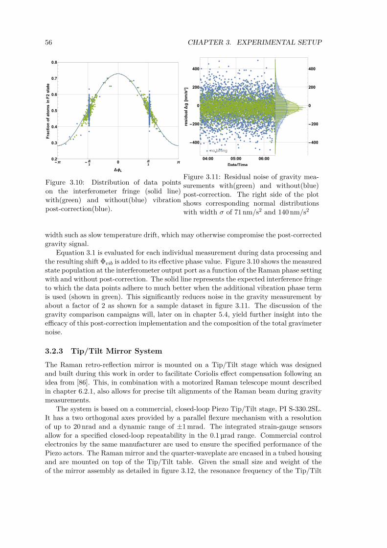
56 CHAPTER 3. EXPERIMENTAL SETUP
Figure 3.10: Distribution of data pointson the interferometer fringe (solid line)with(green) and without(blue) vibrationpost-correction(blue).
Figure 3.11: Residual noise of gravity mea-surements with(green) and without(blue)post-correction. The right side of the plotshows corresponding normal distributionswith width σ of 71 nm/s2 and 140 nm/s2
width such as slow temperature drift, which may otherwise compromise the post-correctedgravity signal.
Equation 3.1 is evaluated for each individual measurement during data processing andthe resulting shift Φvib is added to its effective phase value. Figure 3.10 shows the measuredstate population at the interferometer output port as a function of the Raman phase settingwith and without post-correction. The solid line represents the expected interference fringeto which the data points adhere to much better when the additional vibration phase termis used (shown in green). This significantly reduces noise in the gravity measurement byabout a factor of 2 as shown for a sample dataset in figure 3.11. The discussion of thegravity comparison campaigns will, later on in chapter 5.4, yield further insight into theefficacy of this post-correction implementation and the composition of the total gravimeternoise.
3.2.3 Tip/Tilt Mirror SystemThe Raman retro-reflection mirror is mounted on a Tip/Tilt stage which was designedand built during this work in order to facilitate Coriolis effect compensation following anidea from [86]. This, in combination with a motorized Raman telescope mount describedin chapter 6.2.1, also allows for precise tilt alignments of the Raman beam during gravitymeasurements.
The system is based on a commercial, closed-loop Piezo Tip/Tilt stage, PI S-330.2SL.It has a two orthogonal axes provided by a parallel flexure mechanism with a resolutionof up to 20 nrad and a dynamic range of ±1 mrad. The integrated strain-gauge sensorsallow for a specified closed-loop repeatability in the 0.1 µrad range. Commercial controlelectronics by the same manufacturer are used to ensure the specified performance of thePiezo actors. The Raman mirror and the quarter-waveplate are encased in a tubed housingand are mounted on top of the Tip/Tilt table. Given the small size and weight of theof the mirror assembly as detailed in figure 3.12, the resonance frequency of the Tip/Tilt
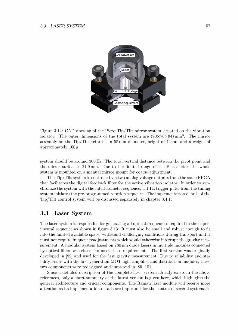
3.3. LASER SYSTEM 57
/4 waveplate
Mirror
Piezo Tip/Tilt stage
Coarse adjustment
Figure 3.12: CAD drawing of the Piezo Tip/Tilt mirror system situated on the vibrationisolator. The outer dimensions of the total system are (90×76×94)mm3. The mirrorassembly on the Tip/Tilt actor has a 55 mm diameter, height of 42 mm and a weight ofapproximately 160 g.
system should be around 300 Hz. The total vertical distance between the pivot point andthe mirror surface is 21.9 mm. Due to the limited range of the Piezo actor, the wholesystem is mounted on a manual mirror mount for coarse adjustment.
The Tip/Tilt system is controlled via two analog voltage outputs from the same FPGAthat facilitates the digital feedback filter for the active vibration isolator. In order to syn-chronize the system with the interferometer sequence, a TTL trigger pulse from the timingsystem initiates the pre-programmed rotation sequence. The implementation details of theTip/Tilt control system will be discussed separately in chapter 3.4.1.
3.3 Laser SystemThe laser system is responsible for generating all optical frequencies required in the exper-imental sequence as shown in figure 3.13. It must also be small and robust enough to fitinto the limited available space, withstand challenging conditions during transport and itmust not require frequent readjustments which would otherwise interrupt the gravity mea-surement. A modular system based on 780 nm diode lasers in multiple modules connectedby optical fibers was chosen to meet these requirements. The first version was originallydeveloped in [82] and used for the first gravity measurement. Due to reliability and sta-bility issues with the first generation MOT light amplifier and distribution modules, thesetwo components were redesigned and improved in [80, 101].
Since a detailed description of the complete laser system already exists in the abovereferences, only a short summary of the latest version is given here, which highlights thegeneral architecture and crucial components. The Raman laser module will receive moreattention as its implementation details are important for the control of several systematic

58 CHAPTER 3. EXPERIMENTAL SETUP
266..
65 M
Hz15
6.95 M
Hz72
.22
MHz
22.8 MHz
700.00 MHz
52S1/2
384
230
484.
47 M
Hz
780.
241n
m
F'=3
F'=2
F'=1
F'=0
F=2
F=1
Ref
eren
ce
MO
T-A
uppe
r trip
let (
poin
ts d
ownw
ards
)
MO
T-B
low
er tr
iple
t (po
ints
upw
ards
)
F=2
Blow
away
and
Det
ectio
n
MO
T R
epum
per
F=1
Blow
away
Ram
an M
aste
r
Ram
an S
lave
1086
.49
MH
z68
34.6
8 M
Hz
52P3/2 72.91 MHz
2563
.0M
Hz
Figure 3.13: Rubidium 87 D2 line hyperfine structure with the necessary laser frequenciesfor laser cooling and stimulated Raman transitions for atom interferometry. Frequencyvalues adopted from [100] and color-coded in agreement with other figures in this document
.
effects. All optical frequencies required during the experimental sequence, as depicted infigure 3.13, are generated using 5 laser sources in distinct modules connected by opticalfibers as shown in figure 3.14.
Reference Laser This module provides the optical frequency reference to which all otherlasers (except the Raman slave) are directly phase-locked with freely adjustableoffset frequencies [82]. This architecture ensures at the same time optimal flexibilityand accuracy in terms of frequency control. The spectroscopy module contains anexternal cavity diode laser (ECDL) and a Rb spectroscopy cell and is frequency-locked to the 85Rb D2 F3 → F′4 line using modulation transfer spectroscopy (MTS)[102]. Together with a 40 MHz offset due to an internal AOM this leads to an opticalfrequency of 1086.69 MHz above the 87Rb D2 F2 → F′3 transition.
Cooling Laser light for the MOT telescopes is generated by a distributed feedback(DFB) laser diode frequency stabilized around the 52S1/2 F = 2 → F′ = 3 transition.

3.3. LASER SYSTEM 59
Repu
mp
Blow
away
Dete
ction
Reference Laser
CoolingLaser
TATA
RepumperLaser
MOT-B + RepumperAOM Switching
MOT-AAOM Switching
MOT-ADistribution
MOT-BDistribution
RamanMaster
RamanSlave
TATA TATA
Lock Lock
Ram
an M
aste
r+Sl
ave
Lock
Detection Region MOT Telescopes Raman Telescope
Figure 3.14: Structure of the GAIN laser system. Boxes correspond to separate lasermodules connected by optical fibers with colors indicating the same optical frequencies asdepicted in 3.13.
Its output is amplified by one separate 2 W tapered amplifier (TA) module whichdelivers a fiber-coupled output power of almost 1 W [101]. This results in a powerof approximately 50 mW per beam in the vacuum chamber, which corresponds toroughly one saturation intensity for the large 30 mm 1/e2 MOT beam diameter. Inorder to facilitate the moving-molasses launch sequence, the upper(A) and lower(B)MOT beam triplets need a relative frequency shift implemented using two separatemodules with single-pass AOMs used for both frequency shifting and intensity/pulsecontrol as detailed in [80]. The MOT-B switching module also provides a repumperinput and auxiliary output fibers for detection, blow-away and repump beams. Twopurely passive distribution modules with one input and three outputs then deliver atotal of six optical fibers to the MOT telescopes.
Repump Laser As the cooling transition of 87Rb is not fully closed, atoms get lost fromthe cooling cycle through decay to the F = 1 ground state. This laser drives the52S1/2 F = 1 → F′ = 2 transition from where the atoms can decay back to the F = 2ground state which returns them to the cooling cycle. The light is generated by aDFB diode laser which delivers a approximately 10 mw each to the MOT-repump-and the detection-fiber, which is more than enough. Originally it was also coupledinto the MOT-B fibers which was later removed, however, since it reduced the coolingpower efficiency in the MOT-B path with the current switching module design [80].In order to facilitate blow-away pulses for atoms in the lower hyperfine ground statethe repump laser can quickly be tuned to the F1 → F′0 cycling transition.
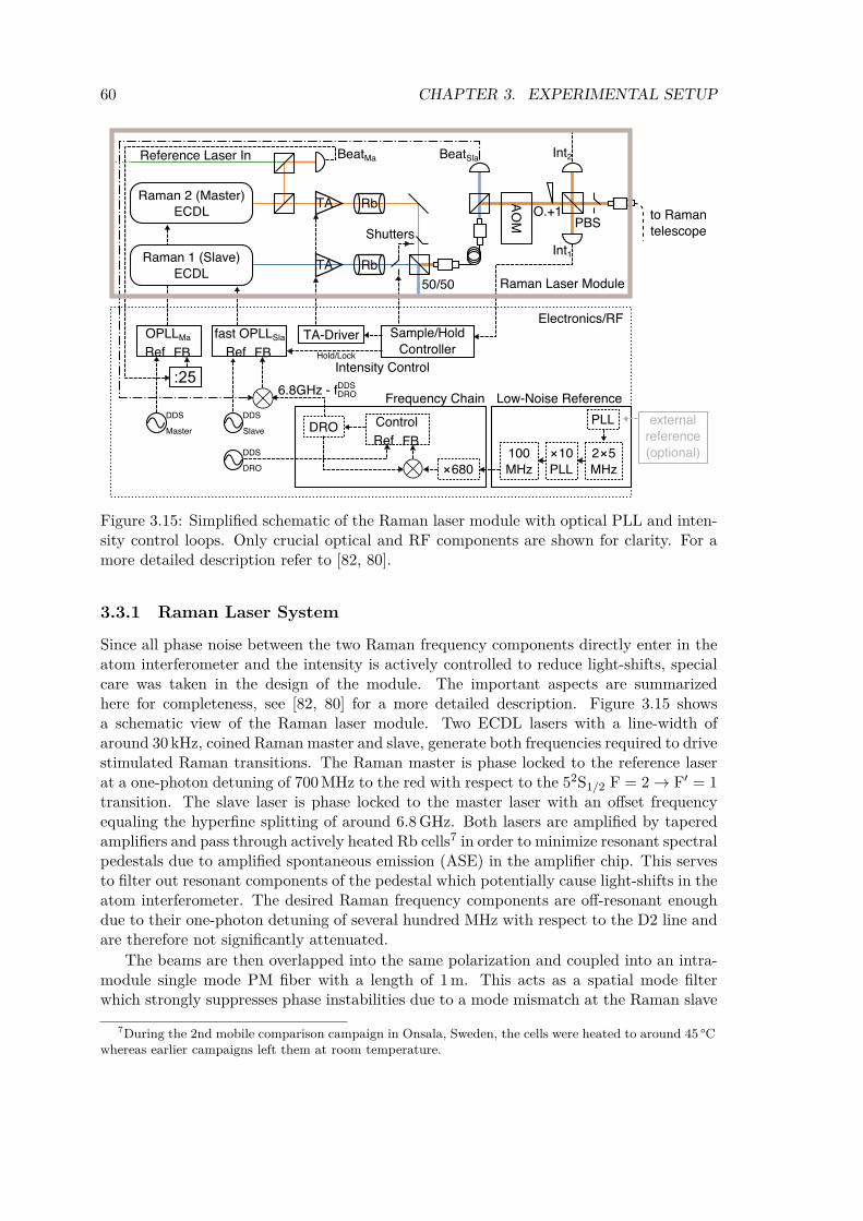
60 CHAPTER 3. EXPERIMENTAL SETUP
Sample/Hold
Controllerfast OPLLSla
Ref FB
OPLLMa
Ref FB
TA-Driver
:25Low-Noise ReferenceFrequency Chain
Control
Ref FB
Intensity Control
DRO
Hold/Lock
Electronics/RF
Raman Laser Module
PBS
50/50
⨯680
6.8GHz - fDRODDS
DDS
Slave
100
MHz
⨯10
PLL
2⨯5
MHz
PLL external
reference
(optional)
DDS
Master
DDS
DRO
Raman 2 (Master)
ECDL
Raman 1 (Slave)
ECDL
Rb
Shutters
AO
M
TA
TA
Rb
Reference Laser In BeatMa BeatSla Int2
O.+1
Int1
to Raman
telescope
Figure 3.15: Simplified schematic of the Raman laser module with optical PLL and inten-sity control loops. Only crucial optical and RF components are shown for clarity. For amore detailed description refer to [82, 80].
3.3.1 Raman Laser System
Since all phase noise between the two Raman frequency components directly enter in theatom interferometer and the intensity is actively controlled to reduce light-shifts, specialcare was taken in the design of the module. The important aspects are summarizedhere for completeness, see [82, 80] for a more detailed description. Figure 3.15 showsa schematic view of the Raman laser module. Two ECDL lasers with a line-width ofaround 30 kHz, coined Raman master and slave, generate both frequencies required to drivestimulated Raman transitions. The Raman master is phase locked to the reference laserat a one-photon detuning of 700 MHz to the red with respect to the 52S1/2 F = 2 → F′ = 1transition. The slave laser is phase locked to the master laser with an offset frequencyequaling the hyperfine splitting of around 6.8 GHz. Both lasers are amplified by taperedamplifiers and pass through actively heated Rb cells7 in order to minimize resonant spectralpedestals due to amplified spontaneous emission (ASE) in the amplifier chip. This servesto filter out resonant components of the pedestal which potentially cause light-shifts in theatom interferometer. The desired Raman frequency components are off-resonant enoughdue to their one-photon detuning of several hundred MHz with respect to the D2 line andare therefore not significantly attenuated.
The beams are then overlapped into the same polarization and coupled into an intra-module single mode PM fiber with a length of 1 m. This acts as a spatial mode filterwhich strongly suppresses phase instabilities due to a mode mismatch at the Raman slave
7During the 2nd mobile comparison campaign in Onsala, Sweden, the cells were heated to around 45 °Cwhereas earlier campaigns left them at room temperature.

3.3. LASER SYSTEM 61
beat-note diode behind the fiber. A single-pass AOM is used behind the fiber for flexiblepulse-shaping during the experimental sequence.
An active intensity stabilization system monitors the power of both beams indepen-dently using a photo diode behind a polarizing beam splitter (PBS) in order to compensatefor slow power drifts. Since both beams are already overlapped in the same spatial andpolarization mode at this point, two alternating shutters in front of the beam combiner areused to measure the master and slave intensity periodically between experimental runs.A sample-and-hold controller then adjusts the TA current to stabilize the beam powersaround the set-points. A second photo-diode on the other PBS side measures the power re-turning from the physics-package which is used for the active retro-reflection stabilizationas detailed in chapter 6.2.1.
The Raman slave optical PLL is a custom design from [82] and features a HF modu-lation circuit to achieve a large control bandwidth of around 4 MHz to avoid phase noisein the frequency band of 0.1–60 kHz where the interferometer is most sensitive accordingto the transfer function shown in figure 2.4.
A schematic of the phase lock architecture is shown in figure 3.15 and explained infull detail in [82]. Since most low-noise phase-frequency detectors (PFDs) do not workat frequencies as high as 6.8 GHz, the Raman beat is first down-converted to a lowerfrequency using the output of a dielectric resonator oscillator (DRO) which is phase-locked to a 6.8 GHz signal with a variable offset fDRO. It is part of an integrated frequencymultiplication chain designed and built by the group of A. Landragin at SYRTE, Paris[99]. This results in a beat frequency between Raman master and slave given by the simpleformula
fBeatSla =
ω12
2π= fDRO + fDDS
PFD = 6.8 GHz − fDDSDRO + fDDS
PFD (3.2)
where fDRO and fPFD are created by two independent direct digital synthesizer (DDS) andcan be controlled at will during the interferometer sequence as detailed in chapter 3.4.2.Note that the DRO has a limited electrical tuning range of approximately (6745±10)MHzwhich limits the practical values of fDDS
DRO at the current mechanical tuning to around(55±10)MHz. For the standard setting fDDS
PFD = 90 MHz the Raman resonance conditionfor atoms at rest is met at fDDS
DRO ≊ 55.317 MHz. Note that, because of the variable DROfrequency, the reference input of the Raman slave PLL can be left constant during theentire Raman frequency chirp which compensates for the atomic Doppler shift during thesequence. This circumvents problems due to potential frequency dependent PLL phaseshifts which could otherwise cause systematic offsets in the gravimeter measurement.
Since DRO phase noise will directly enter in the atom interferometer phase, a low-noisefrequency reference is used as an input to the multiplication chain. Due to its importanceand because it also serves as a reference oscillator for all other parts of the GAIN setupthis will be discussed in more detail in the next chapter.
Frequency Reference
All radio frequencies used in the experiment, including the frequency difference of theRaman lasers, are ultimately derived from the low-noise frequency reference depicted inthe bottom right of figure 3.15. In order to not limit gravimeter performance by noisesources in this reference or other elements in the frequency chain great care was taken toensure that the chosen components meet the required noise specifications [82, 93]. Since nosingle quartz oscillator fulfills the noise specifications at both low and high frequencies, a
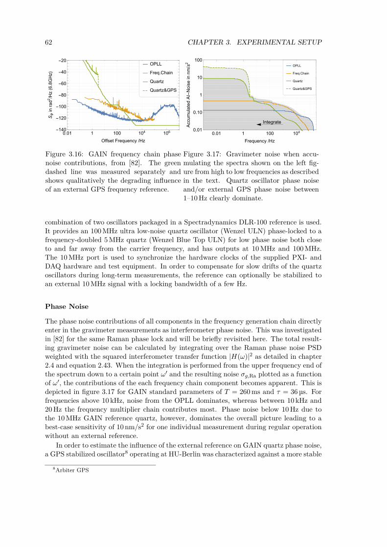
62 CHAPTER 3. EXPERIMENTAL SETUP
OPLL
Freq.Chain
Quartz
Quartz&GPS
0.01 1 100 104 106-140-120-100-80-60-40-20
Offset Frequency /Hz
Sinrad2/Hz(
6.8GHz)
Figure 3.16: GAIN frequency chain phasenoise contributions, from [82]. The greendashed line was measured separately andshows qualitatively the degrading influenceof an external GPS frequency reference.
OPLL
Freq.Chain
Quartz
Quartz&GPS
0.01 1 100 1040.01
0.10
1
10
100
Frequency /Hz
AccumulatedAI-No
iseinnm
/s2
Integrate
Figure 3.17: Gravimeter noise when accu-mulating the spectra shown on the left fig-ure from high to low frequencies as describedin the text. Quartz oscillator phase noiseand/or external GPS phase noise between1–10 Hz clearly dominate.
combination of two oscillators packaged in a Spectradynamics DLR-100 reference is used.It provides an 100 MHz ultra low-noise quartz oscillator (Wenzel ULN) phase-locked to afrequency-doubled 5 MHz quartz (Wenzel Blue Top ULN) for low phase noise both closeto and far away from the carrier frequency, and has outputs at 10 MHz and 100 MHz.The 10 MHz port is used to synchronize the hardware clocks of the supplied PXI- andDAQ hardware and test equipment. In order to compensate for slow drifts of the quartzoscillators during long-term measurements, the reference can optionally be stabilized toan external 10 MHz signal with a locking bandwidth of a few Hz.
Phase Noise
The phase noise contributions of all components in the frequency generation chain directlyenter in the gravimeter measurements as interferometer phase noise. This was investigatedin [82] for the same Raman phase lock and will be briefly revisited here. The total result-ing gravimeter noise can be calculated by integrating over the Raman phase noise PSDweighted with the squared interferometer transfer function |H(ω)|2 as detailed in chapter2.4 and equation 2.43. When the integration is performed from the upper frequency end ofthe spectrum down to a certain point ω′ and the resulting noise σg,Ra plotted as a functionof ω′, the contributions of the each frequency chain component becomes apparent. This isdepicted in figure 3.17 for GAIN standard parameters of T = 260 ms and τ = 36 µs. Forfrequencies above 10 kHz, noise from the OPLL dominates, whereas between 10 kHz and20 Hz the frequency multiplier chain contributes most. Phase noise below 10 Hz due tothe 10 MHz GAIN reference quartz, however, dominates the overall picture leading to abest-case sensitivity of 10 nm/s2 for one individual measurement during regular operationwithout an external reference.
In order to estimate the influence of the external reference on GAIN quartz phase noise,a GPS stabilized oscillator8 operating at HU-Berlin was characterized against a more stable
8Arbiter GPS
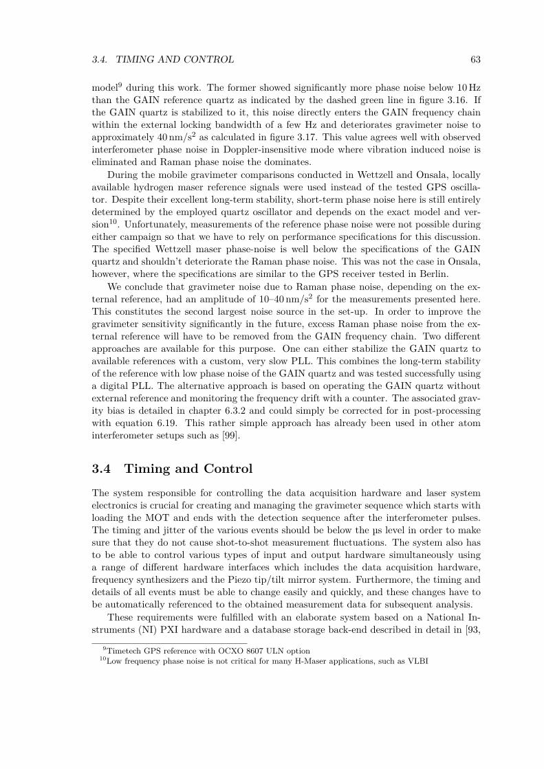
3.4. TIMING AND CONTROL 63
model9 during this work. The former showed significantly more phase noise below 10 Hzthan the GAIN reference quartz as indicated by the dashed green line in figure 3.16. Ifthe GAIN quartz is stabilized to it, this noise directly enters the GAIN frequency chainwithin the external locking bandwidth of a few Hz and deteriorates gravimeter noise toapproximately 40 nm/s2 as calculated in figure 3.17. This value agrees well with observedinterferometer phase noise in Doppler-insensitive mode where vibration induced noise iseliminated and Raman phase noise the dominates.
During the mobile gravimeter comparisons conducted in Wettzell and Onsala, locallyavailable hydrogen maser reference signals were used instead of the tested GPS oscilla-tor. Despite their excellent long-term stability, short-term phase noise here is still entirelydetermined by the employed quartz oscillator and depends on the exact model and ver-sion10. Unfortunately, measurements of the reference phase noise were not possible duringeither campaign so that we have to rely on performance specifications for this discussion.The specified Wettzell maser phase-noise is well below the specifications of the GAINquartz and shouldn’t deteriorate the Raman phase noise. This was not the case in Onsala,however, where the specifications are similar to the GPS receiver tested in Berlin.
We conclude that gravimeter noise due to Raman phase noise, depending on the ex-ternal reference, had an amplitude of 10–40 nm/s2 for the measurements presented here.This constitutes the second largest noise source in the set-up. In order to improve thegravimeter sensitivity significantly in the future, excess Raman phase noise from the ex-ternal reference will have to be removed from the GAIN frequency chain. Two differentapproaches are available for this purpose. One can either stabilize the GAIN quartz toavailable references with a custom, very slow PLL. This combines the long-term stabilityof the reference with low phase noise of the GAIN quartz and was tested successfully usinga digital PLL. The alternative approach is based on operating the GAIN quartz withoutexternal reference and monitoring the frequency drift with a counter. The associated grav-ity bias is detailed in chapter 6.3.2 and could simply be corrected for in post-processingwith equation 6.19. This rather simple approach has already been used in other atominterferometer setups such as [99].
3.4 Timing and ControlThe system responsible for controlling the data acquisition hardware and laser systemelectronics is crucial for creating and managing the gravimeter sequence which starts withloading the MOT and ends with the detection sequence after the interferometer pulses.The timing and jitter of the various events should be below the µs level in order to makesure that they do not cause shot-to-shot measurement fluctuations. The system also hasto be able to control various types of input and output hardware simultaneously usinga range of different hardware interfaces which includes the data acquisition hardware,frequency synthesizers and the Piezo tip/tilt mirror system. Furthermore, the timing anddetails of all events must be able to change easily and quickly, and these changes have tobe automatically referenced to the obtained measurement data for subsequent analysis.
These requirements were fulfilled with an elaborate system based on a National In-struments (NI) PXI hardware and a database storage back-end described in detail in [93,
9Timetech GPS reference with OCXO 8607 ULN option10Low frequency phase noise is not critical for many H-Maser applications, such as VLBI
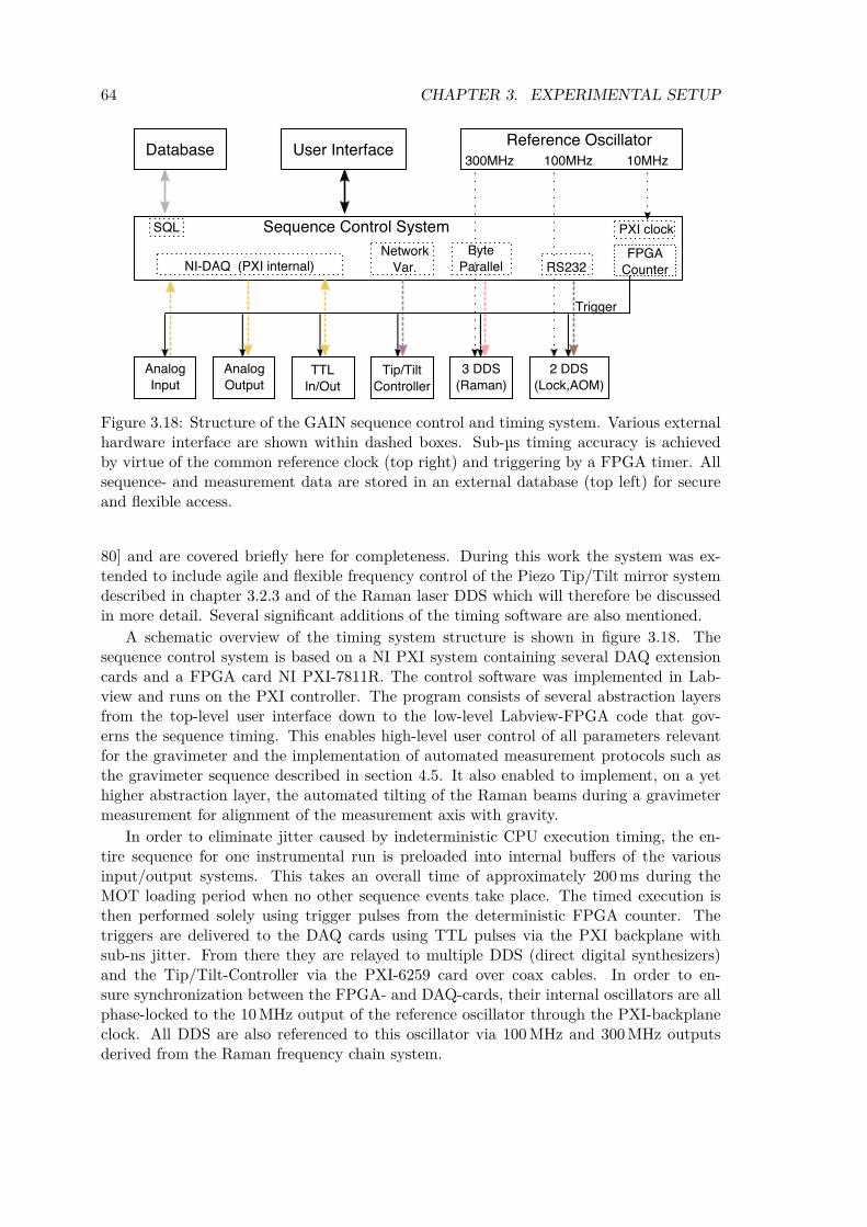
64 CHAPTER 3. EXPERIMENTAL SETUP
FPGA
Counter
Sequence Control System
Trigger
NI-DAQ (PXI internal)Network
Var.
Byte
Parallel RS232
Reference Oscillator300MHz 100MHz 10MHz
User InterfaceDatabase
SQL PXI clock
Analog
Input
Analog
OutputTTL
In/Out
2 DDS
(Lock,AOM)Tip/Tilt
Controller
3 DDS
(Raman)
Figure 3.18: Structure of the GAIN sequence control and timing system. Various externalhardware interface are shown within dashed boxes. Sub-µs timing accuracy is achievedby virtue of the common reference clock (top right) and triggering by a FPGA timer. Allsequence- and measurement data are stored in an external database (top left) for secureand flexible access.
80] and are covered briefly here for completeness. During this work the system was ex-tended to include agile and flexible frequency control of the Piezo Tip/Tilt mirror systemdescribed in chapter 3.2.3 and of the Raman laser DDS which will therefore be discussedin more detail. Several significant additions of the timing software are also mentioned.
A schematic overview of the timing system structure is shown in figure 3.18. Thesequence control system is based on a NI PXI system containing several DAQ extensioncards and a FPGA card NI PXI-7811R. The control software was implemented in Lab-view and runs on the PXI controller. The program consists of several abstraction layersfrom the top-level user interface down to the low-level Labview-FPGA code that gov-erns the sequence timing. This enables high-level user control of all parameters relevantfor the gravimeter and the implementation of automated measurement protocols such asthe gravimeter sequence described in section 4.5. It also enabled to implement, on a yethigher abstraction layer, the automated tilting of the Raman beams during a gravimetermeasurement for alignment of the measurement axis with gravity.
In order to eliminate jitter caused by indeterministic CPU execution timing, the en-tire sequence for one instrumental run is preloaded into internal buffers of the variousinput/output systems. This takes an overall time of approximately 200 ms during theMOT loading period when no other sequence events take place. The timed execution isthen performed solely using trigger pulses from the deterministic FPGA counter. Thetriggers are delivered to the DAQ cards using TTL pulses via the PXI backplane withsub-ns jitter. From there they are relayed to multiple DDS (direct digital synthesizers)and the Tip/Tilt-Controller via the PXI-6259 card over coax cables. In order to en-sure synchronization between the FPGA- and DAQ-cards, their internal oscillators are allphase-locked to the 10 MHz output of the reference oscillator through the PXI-backplaneclock. All DDS are also referenced to this oscillator via 100 MHz and 300 MHz outputsderived from the Raman frequency chain system.
3.4. TIMING AND CONTROL 65
All voltage input and output channels are provided by two PXI-6723 and one PXI-6259data acquisition (DAQ) cards. This results in a total of 24×16 bit input channels for timed1 Msps data acquisition and 64×16 bit output channels with a variable range of up to ±10 Vfor synchronized arbitrary waveform output during the sequence. The output channels areused to control, e.g., AOM diffraction efficiencies using voltage variable attenuators or thecurrent drivers sourcing magnetic field coils on the physics package. Additionally, 32external TTL signal channels are used, e.g., to control fast RF-pulse switches in the AOMsignal paths and to deliver trigger pulses to the laser shutter drivers, Tip/Tilt mirror, MOTcameras, DDS and other subsystems. All channels are delivered through coax BNC- orSMA-cables via a custom-built signal breakout box which contains additional functionsfor some channels such as shutter drivers or active impedance converters.
Two Novatech 409b DDS11 provide a total of 8 independent RF signals for the cooling-and repump laser PLL reference and for all AOMs in the GAIN laser system. Their internaloscillators are locked to the 100 MHz GAIN low-noise reference oscillator as shown in figure3.18. Since the programming interface to the timing system is a comparatively slow RS232connection, all frequency-, phase- and amplitude-values required during the sequence arepreloaded into an internal 4MB ”Table Mode” buffer prior to each measurement run.After optimizations of the serial communication conducted during this work, the completeprogramming of both DDS now takes less than 150 ms and can easily be done during theMOT loading phase without constraining the experimental cycle time.
All sequence information and recorded measurement data is simultaneously sent acrossthe network to a MySQL database server contained in the GAIN setup as indicated inthe top left corner of figure 3.18. The database layout is described in detail in [80]. Thisguarantees direct, convenient and secure data access with the ability to run complex dataqueries. To ensure data safety, the experiment data is furthermore replicated on a second,remote database server at Humboldt Universität zu Berlin.
3.4.1 Tip/Tilt Mirror ControlSweeps of the Piezo Tip/Tilt mirror described in chapter 3.2.3 implement both the Cori-olis compensation and Raman beam auto-collimation via sweeps along two perpendicularaxes during both Ramam interferometer- and the auxiliary pulse-sequence as detailed inchapters 6.2.1 and 6.1.1. In order to guarantee deterministic high-level control over thesesweeps, a Tip/Tilt steering system was developed during this work as described below.
Two analog voltage inputs of the closed-loop Piezo controller are used to facilitatearbitrary steering of the Tip/Tilt system. They control the internal feedback loop set-points and are thus not subjected to hysteresis, drift or other spurious Piezo effects. Due tothe proximity to the vibration isolator, the simplest way to access the set-points digitally isby using two analog outputs of the existing compactRIO system which already implementsthe active vibration feedback filter. Since the compactRIO is clocked by its own internaloscillator, a synchronization to the rest of the timing system is necessary and performedusing a TTL trigger pulse at the start of each experimental cycle. The Tip/Tilt steeringis then implemented using a deterministic FPGA program running on the compactRIOwhich gradually changes both control voltages.
In order to facilitate a flexible but high-level control by the user, input to this programis a list of chirp segments each containing the timing and voltage and ramp values for
11based on Analog Devices AD9959 ICs

66 CHAPTER 3. EXPERIMENTAL SETUP
Chirp Segmentst1 fit2 fi
:
DDSDDS
Timing Software FIFObuffer FPGA
ControlNI PXI-7811R
22 bitparallel LVDS linkSerializer
DS90UR241Q
Demux:4 18 bitparallel
DeserializerDS90UR124Q
DDS8mMaster
DDS
DDS8mSlave
DDS8mDRO
Segment Triggers(IOUD TTL)
Figure 3.19: Schematic of the implemented byte-parallel Raman DDS control system.Linear chirp segments (see text) are computed by the timing software and implementedby an FPGA which controls up to four DDS8m via a fast, serial LVDS link. In order toavoid the small serialization delay, the time critical trigger signals are delivered to eachDDS using standard coax connections.
both channels. The program adheres to the requested time-/voltage(s)-values and realizesa simple linear interpolation in between. Due to the comparatively high sampling rateof 20 kHz this implements a quasi-continuous Tip/Tilt sweep. Note that continuity andsmoothness over the whole sequence, and not just during the interferometer pulses, is rel-evant here to minimize the torque on the vibration platform. Step-like mirror movementsduring tests, on the other hand, heavily interfered with the active feedback system anddrove it beyond its dynamic range. Due to the automatic continuous sweep, however, nosuch interference has been observed even on the seismically quietest sites and is thereforenot a problem.
The user interface provides a higher-level representation which allows to enter theorientation of the tip/tilt system relative to the geographic reference frame. Tip/tiltvalues and sweep rates along NS and EW axes can then be entered directly for both theRaman interferometer- and the pseudo-pulses-interval during the MOT-phase. The chirpsegment list is computed from these specifications by the sequence control system andtransfered to the compactRIO via Ethernet before the start of each experimental cycle.
3.4.2 Agile Raman DDS Control
The Raman laser phase locks are referenced to a total of three DDS which are labeled mas-ter, slave and DRO as shown in figure 3.15. In order to implement µHz level frequencycontrol and fine tuning of the chirp rate, Novatech DDS408A/DDS8m synthesizers with48 bit wide frequency control registers are used. They are clocked by 300 MHz signals di-rectly derived from the Raman frequency generation chain for synchronization and reducedphase noise compared to internal oscillator operation.
Since these synthesizers do not have an on-board buffer for multiple output settingsthey need to be reprogrammed within the experimental sequence to change the Ramanfrequency in a flexible manner for all but the simplest tasks. For example, before theimplementation of this system the Raman frequency could not be chirped during the longvelocity selection pulse leading to potential smearing of the selected velocity class. Asthe standard RS232 interface takes at least 50 ms to transmit every command, which is
3.4. TIMING AND CONTROL 67
much too slow for agile frequency control, a faster interface was implemented as part ofthis work and depicted in figure 3.19. It is based on a 24-pin connector on the DDS PCBwhich allows direct access to all relevant registers inside the AD9854 synthesizer IC usingonly 18 pins. This enables full, real-time control over the output frequency, amplitude andphase. In order to set these registers reliably and quickly, the same FPGA board is usedthat implements the sequence timing. Since all three involved DDS need to be accessedonly sequentially and not in parallel, multiplexer/demultiplexer boards were realized usingelectronic latches. They enable the addressing of up to four DDS sequentially using onlyone output with 18 + 4pins. In order to remove the need for long unwieldy shieldedparallel signal cables between the FPGA and the DDS, which are located in differentparts of the GAIN setup, a data serialization system was furthermore implemented on theMux/Demux board together with Eugen Dischke. It is based on low voltage differentialsignaling (LVDS) ICs and provides a real-time and low-latency12 compression of all signallines onto one twisted-pair wire, such as e.g. in a standard Ethernet cable. The powerusage of the serialization system is low enough that it can be sourced from the FPGA itselfand it is clocked using a 10 MHz signal derived from the FPGA as well. At the currentFPGA clock rate of 10 MHz and without optimization the interface is capable of writingtwo bytes to the DDS buffer within 6 clock cycles, or 0.6 µs. This is more than 5 orders ofmagnitude faster than the previous RS232 interface and enables a complete rewrite of allDDS registers (which is almost never necessary) within less than 5 µs. According to theDDS8m specifications, this could theoretically be accelerated in the future by yet anotherorder of magnitude to less than 25 ns per byte.
The programing format used to realize the desired DDS behavior is based on theAD9854 frequency chirp mode and closely related to the tilt chirp program implementedfor the Tip/Tilt mirror13: A list of chirp segments with time/frequency value pairs is sentto the FPGA before the beginning of the sequence. The FPGA realizes these values byprogramming the AD9854 using one appropriate start frequency and the sequential chirprate values together with their respective timings during the sequence. In order to activateeach chirp segment at exactly the right clock cycle, the parameters of the next segment arewritten to the AD9854 input buffers during the previous segment. A positive edge on thetrigger input then causes the buffered values to be written to the DDS working registersimmediately. To avoid potential jitters of the trigger signal due to the serialization systemdelay, this single line is delivered to the DDS directly through a standard coax connection(identical to the previous RS232 method). Note that this timing scheme only works ifboth FPGA and DDS are synchronized by the same clock as shown in figure 3.18, sincecycle slips between them will otherwise lead to frequency offsets during the sequence. Inorder to reference the output to a fix starting point, all DDS are reset to a fixed frequencyvalue during the MOT phase of each experimental cycle. To provide the experimenterwith a more meaningful set of control parameters, an abstraction layer was implementedon which an arbitrary number of frequency ramps can be set on each DDS during thesequence. The required parameters for each ramp are frequency value, chirp rate, theexact time at which the frequency value shall be in effect and the ramp start/stop times.The time spacing between individual segments is limited only to a few µs by the time ittakes to rewrite the DDS registers.
This flexible and fast Raman laser control system enables the realization of advanced12The specified serialization/deserialization delay is smaller than 1µs for a 10 MHz transmit clock13In fact, both routines are implemented with the same code through a common ”chirp” parent class.
68 CHAPTER 3. EXPERIMENTAL SETUP
AI sequences such as large-momentum beam splitters, composite pulses or multi-speciesexperiments. It is thus a crucial addition of the setup and significantly enhances itscapabilities for a broad range of future applications.
SummaryThe preceding chapter gave a comprehensive overview of the experimental apparatus, withan emphasis placed on the parts on which the author contributed most during this work.This specifically includes the magnetically shielded MOT chamber, vibration isolationsystem and post-correction implementation, Tip/Tilt mirror system for Coriolis- and tilt-compensation which will be detailed in chapter 6, and the agile Raman frequency controlsystem.
After this detailed hardware description, the next chapter will introduce the gravitymeasurement sequence with a specification of each functional segment.
Chapter 4
Gravimeter Operation
In order to perform accurate and sensitive gravity measurements with an atom interferom-eter, the details of the atomic source preparation, interferometry and detection sequenceare essential. This chapter will therefore give a detailed description of the experimentalsequence that was used for gravimeter operation. Each run of the sequence takes around1.5 s and is repeated back-to-back continuously during the long-term gravity measurementspresented in chapter 5. First, each functional element of the sequence and afterwards themeasurement protocol that was used to conduct the gravity registration will be describedin the following.
The sequence builds on the previous measurement protocol developed in [82, 93, 80]and was improved in order to optimize the stability, sensitivity and reliability of the gravitymeasurements. First, the upgraded DDS programming detailed in chapter 3.4.2 enabledto chirp the Raman laser frequency to compensate for the changing Doppler-shift duringthe velocity selection pulse. The gravity measurement protocol was furthermore amendedwith a feed-forward mechanism to operate the interferometer at exactly half-fringe evenin the presence of large tidal gravity variations, which is important due to a bias in ourdetection system as detailed in chapter 6.6 and in [80]. Finally, a slow feedback loopwas implemented to compensate for slow drifts of the total Raman power which were notaccounted for using the previous intensity stabilization system described in chapter 3.3.1and in [80].
4.1 MOT and Launch
Each experimental run starts by loading atoms from background gas into the MOT for atime of 0.6 s, which will be explained here briefly for completeness. Refer to, e.g., [103, 81]for a more through description. During the MOT phase, the cooling light is red-detuned byabout 23 MHz or around 4 line-widths from the |32S1/2 F = 2⟩ ↔ |52P3/2 F = 3⟩ transition.The total atom number in the MOT has been estimated to roughly 109 by fluorescencemeasurements with the cameras placed around the MOT and using a formula provided in[100]. When loading is complete, the MOT coils are switched off 5 ms before the launch inorder to give eddy currents sufficient time to decay. During this time the atoms are cooledin the optical molasses. In order to accelerate the atoms upwards a relative detuningbetween upper and lower MOT beam triplets of ∆rel = ±3 MHz is applied which transfers
69

70 CHAPTER 4. GRAVIMETER OPERATION
Lorentzian
Gaussian
weighted Gaussian
65.4 65.5 65.6 65.7
100
102
104
106
Raman Laser Frequency Offset / MHz
Atomnumber/a.u
.
Figure 4.1: Raman frequency scan of the velocity selection pulse. The resulting momentumdistribution is Lorentzian and can not strictly be assigned a temperature value [105, 106].A regular Gaussian fit and a weighted fit which neglects the large wings of the distributionyield effective temperatures of 2.4 µK and 1.6 µK, respectively.
the cooled molasses state to a moving frame with a vertical velocity of:
vlaunch =c
ν0
∆relcosα 4.05 m/s (4.1)
where ν0 is the optical frequency of the cooling laser and α is the angle between thecooling beam and vertical, which in 1-1-1 configuration equals cosα = 1/
√3. At the
end of the launch, a far-off-resonance molasses phase optimized for low final temperaturesis used to minimize the expansion of the cloud during the rest of the experiment. Thefinal temperature in this regime is proportional to the quotient of light intensity anddetuning [81, 104]. During the moving molasses state we therefore increase the detuningin several steps to 144 MHz, or around 24 line-widths, and adiabatically ramp down thelight intensity. The repumper light is switched off shortly after the cooling light to makesure that all atoms are in the F = 2 hyperfine state The achieved launch temperaturesare on the order of 3 µK as detailed in the next chapter which is in agreement with theresults from other 87Rb fountains.
4.2 Velocity- and State SelectionAfter the optical molasses beams are switched off, a velocity-selection Raman pulse [7]is used to select atoms in the magnetically insensitive m = 0 sub-state within a narrowthe vertical momentum distribution of the launched cloud. This is necessary to limitthe mean Doppler-detuning of the cloud during the following interferometer pulses. Theresulting low vertical velocity spread of the cloud also simplifies the identification of severalsystematic effects.
A bias magnetic field is applied and a Doppler-sensitive Raman π pulse with a Gaussianpulse width of σt = 12 µs
(1/e2
)is employed to transfer atoms in a narrow velocity class
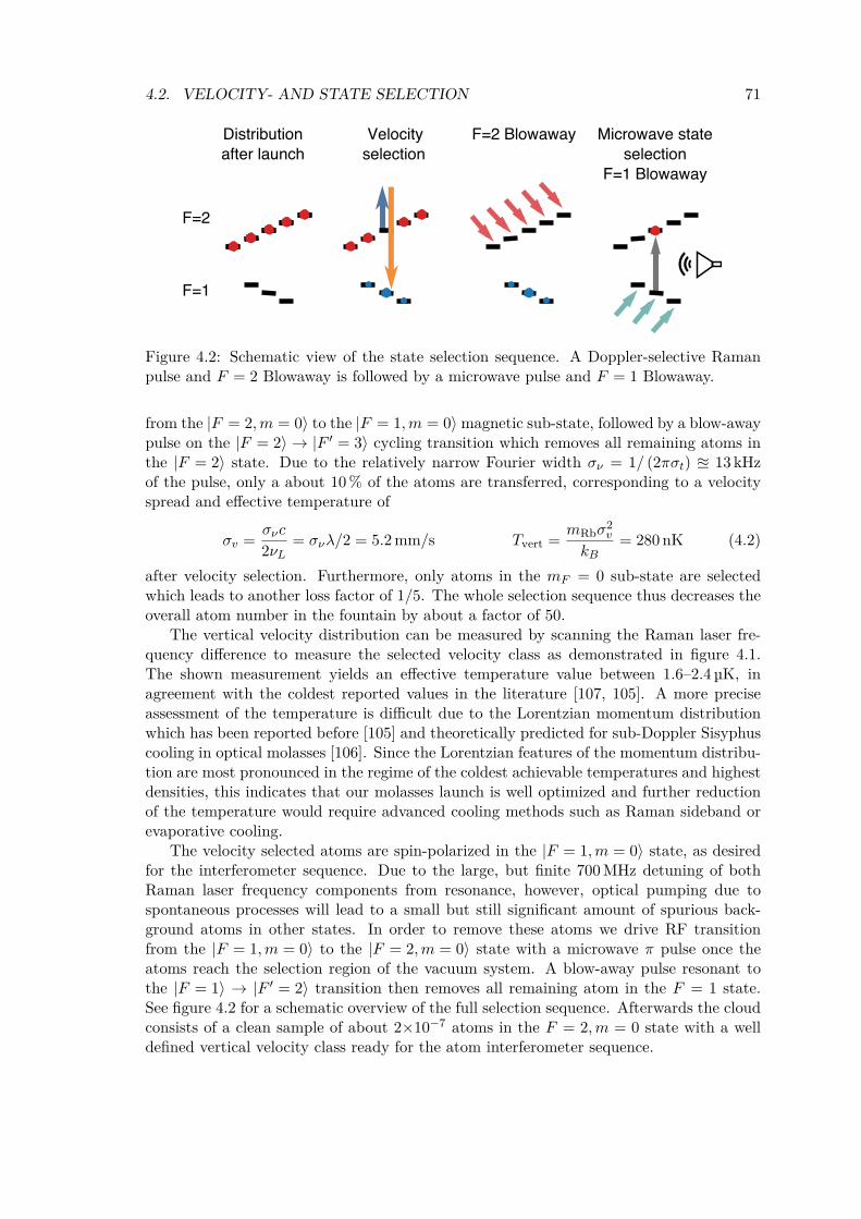
4.2. VELOCITY- AND STATE SELECTION 71
Distributionafter launch
Velocityselection
F=2 Blowaway Microwave stateselection
F=1 Blowaway
F=2
F=1
Figure 4.2: Schematic view of the state selection sequence. A Doppler-selective Ramanpulse and F = 2 Blowaway is followed by a microwave pulse and F = 1 Blowaway.
from the |F = 2,m = 0〉 to the |F = 1,m = 0〉 magnetic sub-state, followed by a blow-awaypulse on the |F = 2〉 → |F ′ = 3〉 cycling transition which removes all remaining atoms inthe |F = 2〉 state. Due to the relatively narrow Fourier width σν = 1/ (2πσt) 13 kHzof the pulse, only a about 10 % of the atoms are transferred, corresponding to a velocityspread and effective temperature of
σv =σνc
2νL= σνλ/2 = 5.2 mm/s Tvert =
mRbσ2v
kB= 280 nK (4.2)
after velocity selection. Furthermore, only atoms in the mF = 0 sub-state are selectedwhich leads to another loss factor of 1/5. The whole selection sequence thus decreases theoverall atom number in the fountain by about a factor of 50.
The vertical velocity distribution can be measured by scanning the Raman laser fre-quency difference to measure the selected velocity class as demonstrated in figure 4.1.The shown measurement yields an effective temperature value between 1.6–2.4 µK, inagreement with the coldest reported values in the literature [107, 105]. A more preciseassessment of the temperature is difficult due to the Lorentzian momentum distributionwhich has been reported before [105] and theoretically predicted for sub-Doppler Sisyphuscooling in optical molasses [106]. Since the Lorentzian features of the momentum distribu-tion are most pronounced in the regime of the coldest achievable temperatures and highestdensities, this indicates that our molasses launch is well optimized and further reductionof the temperature would require advanced cooling methods such as Raman sideband orevaporative cooling.
The velocity selected atoms are spin-polarized in the |F = 1,m = 0〉 state, as desiredfor the interferometer sequence. Due to the large, but finite 700 MHz detuning of bothRaman laser frequency components from resonance, however, optical pumping due tospontaneous processes will lead to a small but still significant amount of spurious back-ground atoms in other states. In order to remove these atoms we drive RF transitionfrom the |F = 1,m = 0〉 to the |F = 2,m = 0〉 state with a microwave π pulse once theatoms reach the selection region of the vacuum system. A blow-away pulse resonant tothe |F = 1〉 → |F ′ = 2〉 transition then removes all remaining atom in the F = 1 state.See figure 4.2 for a schematic overview of the full selection sequence. Afterwards the cloudconsists of a clean sample of about 2×10⁻⁷ atoms in the F = 2,m = 0 state with a welldefined vertical velocity class ready for the atom interferometer sequence.
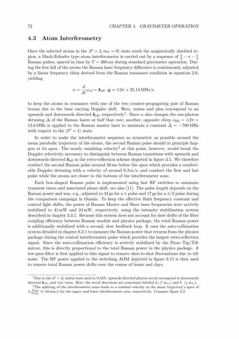
72 CHAPTER 4. GRAVIMETER OPERATION
4.3 Atom Interferometry
Once the selected atoms in the |F = 2,mF = 0⟩ state reach the magnetically shielded re-gion, a Mach-Zehnder type atom interferometer is carried out by a sequence of π
2 − π− π2
Raman pulses, spaced in time by T = 260 ms during standard gravimeter operation. Dur-ing the free fall of the atoms the Raman laser frequency difference is continuously adjustedby a linear frequency chirp derived from the Raman resonance condition in equation 2.6,yielding
α =d
dtω12 = keff · g = ∓2π × 25.14 MHz/s
to keep the atoms in resonance with one of the two counter-propagating pair of Ramanbeams due to the time varying Doppler shift. Here, minus and plus correspond to anupwards and downwards directed keff, respectively1. Since α also changes the one-photondetuning ∆ of the Raman lasers at half that rate, another, opposite chirp αR2 = ±2π ×12.6 MHz is applied to the Raman master laser to maintain a constant ∆ = −700 MHzwith respect to the |F ′ = 1⟩ state.
In order to make the interferometer sequence as symmetric as possible around themean parabolic trajectory of the atoms, the second Raman pulse should in principle hap-pen at its apex. The nearly vanishing velocity2 at this point, however, would break theDoppler selectivity necessary to distinguish between Raman transitions with upwards anddownwards directed keff in the retro-reflection scheme depicted in figure 3.5. We thereforeconduct the second Raman pulse around 30 ms before the apex which provides a comfort-able Doppler detuning with a velocity of around 0.3 m/s, and conduct the first and lastpulse while the atoms are closer to the bottom of the interferometer zone.
Each box-shaped Raman pulse is implemented using fast RF switches to minimizetransient times and associated phase shift, see also [11]. The pulse length depends on theRaman power and was, e.g., adjusted to 34 µs for a π pulse and 17 µs for a π/2 pulse duringthe comparison campaign in Onsala. To keep the effective Rabi frequency constant andcontrol light shifts, the power of Raman Master and Slave laser frequencies were activelystabilized to 41 mW and 24 mW, respectively, using the intensity stabilization systemdescribed in chapter 3.3.1. Because this system does not account for slow drifts of the fibercoupling efficiency between Raman module and physics package, the total Raman poweris additionally stabilized with a second, slow feedback loop. It uses the auto-collimationsystem detailed in chapter 6.2.1 to measure the Raman power that returns from the physicspackage during the central interferometer pulse which provides the largest retro-reflectionsignal. Since the auto-collimation efficiency is actively stabilized by the Piezo Tip/Tiltmirror, this is directly proportional to the total Raman power in the physics package. Alow-pass filter is first applied to this signal to remove shot-to-shot fluctuations due to tiltnoise. The RF power applied to the switching AOM depicted in figure 3.15 is then usedto remove total Raman power drifts over the course of hours and days.
1Due to the |F = 2⟩ initial state used in GAIN, upwards directed photon recoil correspond to downwardsdirected keff, and vice versa. Here, the recoil directions are sometimes labeled k+(↑ vrec) and k (↓ vrec).
2The splitting of the interferometer arms leads to a residual velocity at the mean trajectory’s apex of± ℏkeff
2mRb≊ ±6 mm/s for the upper and lower interferometer arm, respectively. Compare figure 2.2.
4.4. DETECTION 73
/µ
/
NF=2 NTotal NTotal
Repump
Figure 4.3: Fluorescence Detection scheme. The blue line is the signal of the atom cloudwhile the yellow signal was taken 40 ms afterwards and indicates fluorescence from thermalbackground gas. The integral for each pulse is indicated by the blue shaded areas whiledisregarding the slopes. Gray shaded areas show optical pumping from |F = 1〉 to |F = 2〉with repump light.
4.4 Detection
Once the atoms reach the detection region after the end of the interferometry sequence,the internal state population is detected with a pulsed measurement using the fluorescenceimaging system described in chapter 3.1.3. It consists of a sequence of three short detectionbeam pulses as depicted in figure 4.3, during which the laser frequency is set to a −3 MHzred-detuning relative to the F = 2 ↔ F ′ = 3 resonance. During the first pulse witha length of 400 µs only atoms in the |F = 2〉 state contribute to the fluorescence. Asubsequent 10 µs pulse of repump light pumps atoms previously in |F = 1〉 into the upper|F = 2〉 state. The second detection pulse thus induces more fluorescence corresponding tothe total number of atoms. The ratio of the first and second pulse signal area then yieldsthe relative state population PF2 = NF2/NTotal, from which the interferometer phasecan be deduced by inverting equation 2.41. After the second detection pulse, auxiliaryrepump- and detection pulses are carried out for additional time-of-flight information andto test for potential systematic effects.
Noise introduced by the detection system is an important factor and originates froma list of uncorrelated sources. Frequency and intensity fluctuations of the retro-reflecteddetection beam, electronic and PMT noise are potential technical noise sources whichshould be suppressed as much as possible. Additionally, the standard quantum limitprovides a fundamental limitation to the achievable uncertainty of the detected statepopulation σP2 ≥ 1/
√NTotal for a given number of atoms. If a detection system achieves
this limited it is said to be limited by atomic shot noise, which is optimal in the sense thatthe only remaining way to further decrease noise is to increase the atom number.
In order to quantify the amplitude of detection noise in the system the following terms
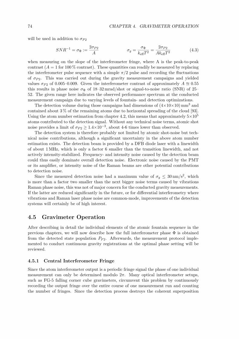
74 CHAPTER 4. GRAVIMETER OPERATION
will be used in addition to σP2
SNR−1 = σΦ :=2σP2
Aσg =
σΦkeffT 2
=2σP2
AkeffT 2(4.3)
when measuring on the slope of the interferometer fringe, where A is the peak-to-peakcontrast (A = 1 for 100 % contrast). These quantities can readily be measured by replacingthe interferometer pulse sequence with a simple π/2 pulse and recording the fluctuationsof σP2. This was carried out during the gravity measurement campaigns and yieldedvalues σP2 of 0.005–0.009. Given the interferometer contrast of approximately A ≊ 0.55this results in phase noise σΦ of 18–32 mrad/shot or signal-to-noise ratio (SNR) of 25–52. The given range here indicates the observed performance spectrum at the conductedmeasurement campaign due to varying levels of fountain- and detection optimizations.
The detection volume during those campaigns had dimensions of (4×10×10)mm3 andcontained about 3 % of the remaining atoms due to horizontal spreading of the cloud [93].Using the atom number estimation from chapter 4.2, this means that approximately 5×10⁵
atoms contributed to the detection signal. Without any technical noise terms, atomic shotnoise provides a limit of σP2 ≥ 1.4×10⁻³, about 4-6 times lower than observed.
The detection system is therefore probably not limited by atomic shot-noise but tech-nical noise contributions, although a significant uncertainty in the above atom numberestimation exists. The detection beam is provided by a DFB diode laser with a linewidthof about 1 MHz, which is only a factor 6 smaller than the transition linewidth, and notactively intensity-stabilized. Frequency- and intensity noise caused by the detection beamcould thus easily dominate overall detection noise. Electronic noise caused by the PMTor its amplifier, or intensity noise of the Raman beams are other potential contributionsto detection noise.
Since the measured detection noise had a maximum value of σg ≤ 30 nm/s2, whichis more than a factor two smaller than the next bigger noise terms caused by vibrationsRaman phase noise, this was not of major concern for the conducted gravity measurements.If the latter are reduced significantly in the future, or for differential interferometry wherevibrations and Raman laser phase noise are common-mode, improvements of the detectionsystems will certainly be of high interest.
4.5 Gravimeter OperationAfter describing in detail the individual elements of the atomic fountain sequence in theprevious chapters, we will now describe how the full interferometer phase Φ is obtainedfrom the detected state population PF2. Afterwards, the measurement protocol imple-mented to conduct continuous gravity registrations at the optimal phase setting will bereviewed.
4.5.1 Central Interferometer FringeSince the atom interferometer output is a periodic fringe signal the phase of one individualmeasurement can only be determined modulo 2π. Many optical interferometer setups,such as FG-5 falling corner cube gravimeters, circumvent this problem by continuouslyrecording the output fringe over the entire course of one measurement run and countingthe number of fringes. Since the detection process destroys the coherent superposition

4.5. GRAVIMETER OPERATION 75
T=150msT=200msT=260ms
-30 -20 -10 0 10 20 300.2
0.4
0.6
0.8
1.0
- 0 / Hz
P(F2)
Figure 4.4: Interferometer fringes during a central chirp rate scan for different pulseseparations T . At the central interferometer fringe with the correct chirp rate α0 2π×25.14 MHz/s the measured state population is independent of T . The observed fringecontrast A 0.55 also only shows a slight dependence of T .
of two states, however, this is not an option for atom interferometers. Instead, AIs areusually operated close to the central interferometer fringe by adjusting the frequency chirpα which keeps the Raman laser on resonance with the atomic transition during the atom’sfree fall. At the correct setting this chirp exactly compensates for the gravity induced shiftso that α = keff · g so that the total interferometer phase in equation 2.20 vanishes.
In order to operate on the central, or dark, fringe and keep the interferometer phase Φsmaller than 2π with our standard parameters of T = 260 ms and a total gravity inducedphase of Φ = 1.07×10⁷ rad, the chirp rate α has to be determined with an accuracy of1T 2 = 15 Hz/s. This corresponds to a gravity value uncertainty of 5.8×10⁻⁶ m/s2 which isnon-trivial to predict at an unknown site and affords an independent measurement. Thiscan be done in a straightforward way by altering the time T between pulses which leavesthe interferometer signal constant when operating on the central fringe as shown in figure4.4.
4.5.2 Optimized Mid-Fringe Operation
Once the interferometer operates with the correct chirp-rate it continuously measuresgravity in 20 min sets using a protocol described in the following and in [80]. At thebeginning of each set, a full interferometer fringe is scanned using 32 data points in orderto determine the fringe contrast, amplitude and phase. Given those parameters, themeasurement program then operates the interferometer within the [−π, π] interval aroundthe central fringe maximum at the most sensitive mid-fringe setting, alternating successiveruns between the left and right fringe slope. This optimizes the phase sensitivity of theinterferometer and enables the rejection of slow fringe amplitude- and offset drifts as wellas imperfections in the detection system which lead to small distortions of the fringe signalon the flanges as detailed in chapter 6.6 of [80]. Due to tidal gravity changes, which are
76 CHAPTER 4. GRAVIMETER OPERATION
on the order of 1 µm/s2, the interferometer phase changes by about 1 rad on timescalesbetween 6–12 h. In order to keep the interferometer operating at mid-fringe as describedbefore the phase setting has to be corrected during these slow changes. This is done using aslow software feedback loop with a 30 s integral and weak proportional element to equalizethe amplitude on the left- and right side of the fringe [93]. It proved challenging for thefeedback loop, however, to keep the interferometer phase sufficiently close to the mid-fringepoint during relatively quick gravity changes on spring tide slopes such as shown in figure1.4. Since these large tidal changes can easily be predicted, an additional feed-forwardpath based on a simple, purely synthetic tidal model was therefore implemented duringthis work. The feedback loop thus only needs to compensate for small residual gravitychanges not contained in this model, e.g. due to atmospheric- or loading effects. Theamplitude of these residual variation is at least one order of magnitude smaller at around100 nm/s2 over several days, which can be easily handled by the feedback loop.
Interleaved into the procedure described above is a momentum recoil flip betweenk↑ and k↓ configuration at every second shot. This enables us to identify and cancelsystematics effect such as group delays in the Raman frequency chain as detailed in chapter6.7 with high temporal resolution as demonstrated. Since contrast and amplitude areslightly different for upwards- and downwards directed momentum recoil, separate fringesare scanned for both configurations. The final gravity value in this protocol is derived byaveraging over four consecutive runs containing every possible configuration:
Φfinal =1
4
(Φleft↑ +Φright
↑ +Φleft↓ +Φright
↓
)(4.4)
4.5.3 Gravity Value Extraction and Height TransferRunning the atom interferometer in this measurement protocol for a few days yields thehighly dynamic tidal gravity signal introduced in chapter 1 and shown in figure 1.4. Re-ducing this signal to a constant, site-dependent gravity value using an appropriate modelfor the observed time-dependence is a standard problem in gravimetry as described before.
Tidal models were calculated with the free software Tsoft [47] using model parametersprovided by M. Schilling3 and H. Wziontek4. Residual gravity signals due to atmosphericpressure changes were removed with an admittance factor of about 3 nm/s2/hPa and localpressure recordings. After subtracting the polar-motion correction and transferring thevalue from the effective measurement height given by equation 2.37 to a reference height,one can extract the local gravity value as the mean value of the residual dataset. Smalldifferences due to the individual circumstances during the 4 performed gravity comparisonsare described in detail in chapter 5.3.
SummaryThis chapter gave a detailed account of the experimental sequence and steps taken toextract the gravity value during the mobile gravity measurements presented in chapter 6.Special attention was given to detection noise sources and a measurement scheme designedto reject systematic effects in the atom interferometer, since the accuracy and stability ofthe measured gravity data is a central aspect of this work. The next chapter will present
3Institut für Erdmessung, Leibniz Universität Hannover4Federal Agency for Cartography and Geodesy, Leipzig

4.5. GRAVIMETER OPERATION 77
the result of the conducted gravity measurement and analyze the performance achievedwith respect to other gravimeters during the comparison campaigns.

78 CHAPTER 4. GRAVIMETER OPERATION
Chapter 5
Atomic Gravimetry at GeodeticObservatories
The goal of this work is to optimize and quantify the absolute accuracy and other keyperformance characteristics of GAIN during gravity measurements. Due to the dynamicnature of gravimetric signals this can best be achieved through direct comparisons withother, collocated gravimeters. A total of four gravity comparison campaigns were thereforeconducted between 2012 and 2015 as part of this work and will be presented in detail below.The first two campaigns were carried out in the physics building at HUB and involvedsimultaneous operation over several days of GAIN and a gPhone spring-based relativegravimeter in December 2012, and of GAIN and the FG5X-220 absolute gravimeter inJune 2013.
Since a university building in Berlin is a noisy, suboptimal place for state-of-the-artgravimetry and in order to demonstrate the mobility of the GAIN setup, the following twocampaigns were conducted at designated geodetic reference stations in Wettzell, Bavariain November 2013 and in Onsala, Sweden in February 2015. The superconducting relativegravimeters SG-30 and OSG-054, respectively, served as a reference for the comparisonduring those campaigns in combination with a previously determined absolute gravityvalue. All GAIN measurements were conducted in a team including my co-workers M.Hauth and, with the exception of the last campaign, V. Schkolnik. The data obtainedduring the first three campaigns is also presented in [80, 101] with two notable differ-ences: First, the extensive evaluation of the systematic error budget in chapter 6 enablesthe specification of an absolute gravity value for the last three campaigns including theinstrumental uncertainty. Second, the result of the repeated data analysis presented hereincludes a post-correction of vibrational noise as detailed in chapter 5. Furthermore, keycharacteristics such as the magnitude and origin of the observed measurement noise andtime delays [80] have been revisited giving additional insight.
5.1 Initial Comparisons in BerlinThe first direct comparison between GAIN and another gravimeter was carried out in thelaboratory at HUB from November to December 2012. The gPhone-981 relative spring-based gravimeter from Institut für Erdmessung, Leibniz Universität Hannover (IfE) oper-
1Microg-LaCoste
79
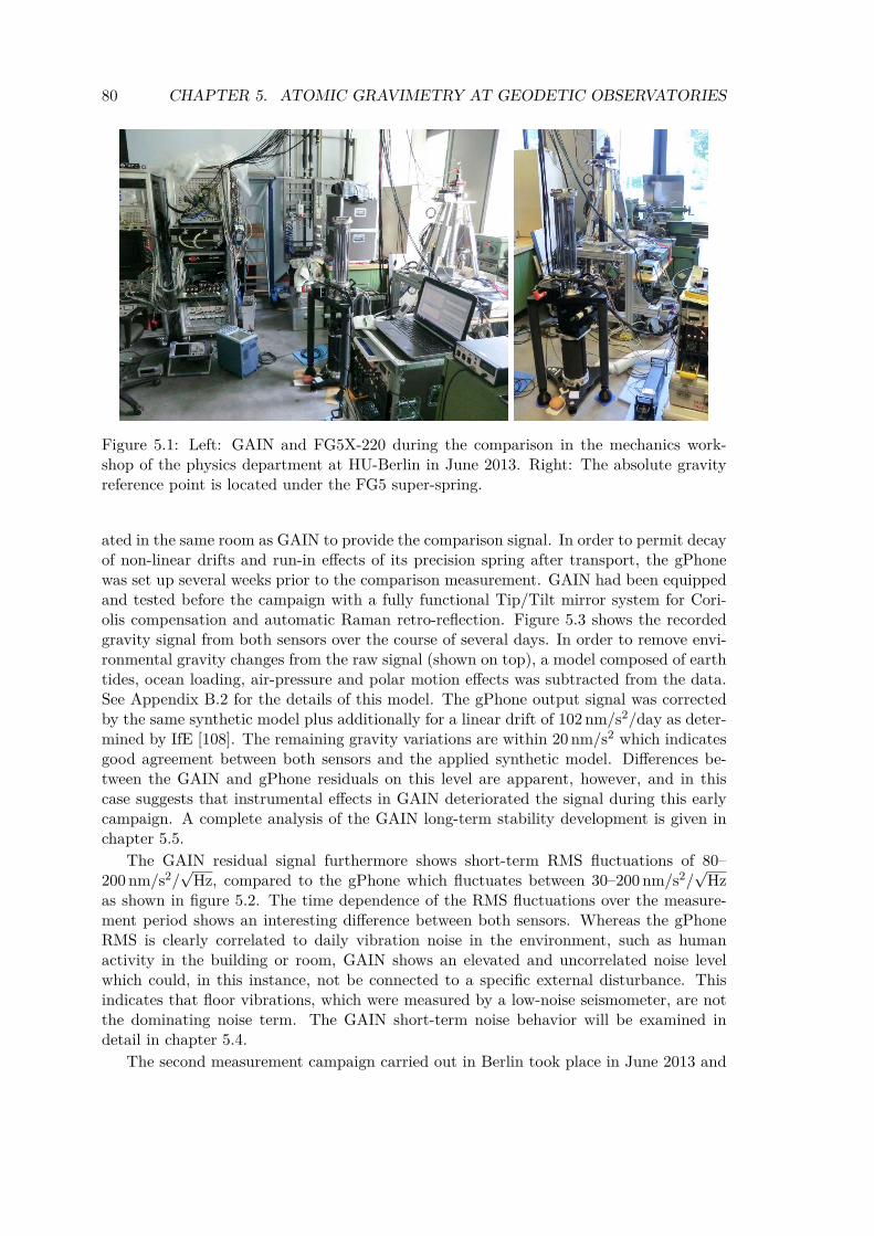
80 CHAPTER 5. ATOMIC GRAVIMETRY AT GEODETIC OBSERVATORIES
Figure 5.1: Left: GAIN and FG5X-220 during the comparison in the mechanics work-shop of the physics department at HU-Berlin in June 2013. Right: The absolute gravityreference point is located under the FG5 super-spring.
ated in the same room as GAIN to provide the comparison signal. In order to permit decayof non-linear drifts and run-in effects of its precision spring after transport, the gPhonewas set up several weeks prior to the comparison measurement. GAIN had been equippedand tested before the campaign with a fully functional Tip/Tilt mirror system for Cori-olis compensation and automatic Raman retro-reflection. Figure 5.3 shows the recordedgravity signal from both sensors over the course of several days. In order to remove envi-ronmental gravity changes from the raw signal (shown on top), a model composed of earthtides, ocean loading, air-pressure and polar motion effects was subtracted from the data.See Appendix B.2 for the details of this model. The gPhone output signal was correctedby the same synthetic model plus additionally for a linear drift of 102 nm/s2/day as deter-mined by IfE [108]. The remaining gravity variations are within 20 nm/s2 which indicatesgood agreement between both sensors and the applied synthetic model. Differences be-tween the GAIN and gPhone residuals on this level are apparent, however, and in thiscase suggests that instrumental effects in GAIN deteriorated the signal during this earlycampaign. A complete analysis of the GAIN long-term stability development is given inchapter 5.5.
The GAIN residual signal furthermore shows short-term RMS fluctuations of 80–200 nm/s2/
√Hz, compared to the gPhone which fluctuates between 30–200 nm/s2/
√Hz
as shown in figure 5.2. The time dependence of the RMS fluctuations over the measure-ment period shows an interesting difference between both sensors. Whereas the gPhoneRMS is clearly correlated to daily vibration noise in the environment, such as humanactivity in the building or room, GAIN shows an elevated and uncorrelated noise levelwhich could, in this instance, not be connected to a specific external disturbance. Thisindicates that floor vibrations, which were measured by a low-noise seismometer, are notthe dominating noise term. The GAIN short-term noise behavior will be examined indetail in chapter 5.4.
The second measurement campaign carried out in Berlin took place in June 2013 and
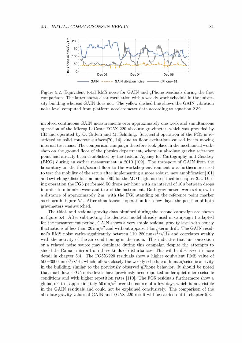
5.1. INITIAL COMPARISONS IN BERLIN 81
//-
Figure 5.2: Equivalent total RMS noise for GAIN and gPhone residuals during the firstcomparison. The latter shows clear correlation with a weekly work schedule in the univer-sity building whereas GAIN does not. The yellow dashed line shows the GAIN vibrationnoise level computed from platform accelerometer data according to equation 2.39.
involved continuous GAIN measurements over approximately one week and simultaneousoperation of the Microg-LaCoste FG5X-220 absolute gravimeter, which was provided byIfE and operated by O. Gitlein and M. Schilling. Successful operation of the FG5 is re-stricted to solid concrete surfaces[70, 14], due to floor excitations caused by its movinginternal test mass. The comparison campaign therefore took place in the mechanical work-shop on the ground floor of the physics department, where an absolute gravity referencepoint had already been established by the Federal Agency for Cartography and Geodesy(BKG) during an earlier measurement in 2010 [109]. The transport of GAIN from thelaboratory on the first/second floor to the workshop environment was furthermore usedto test the mobility of the setup after implementing a more robust, new amplification[101]and switching/distribution module[80] for the MOT light as described in chapter 3.3. Dur-ing operation the FG5 performed 50 drops per hour with an interval of 10 s between dropsin order to minimize wear and tear of the instrument. Both gravimeters were set up witha distance of approximately 2 m, with the FG5 standing on the reference point markeras shown in figure 5.1. After simultaneous operation for a few days, the position of bothgravimeters was switched.
The tidal- and residual gravity data obtained during the second campaign are shownin figure 5.4. After subtracting the identical model already used in campaign 1 adaptedfor the measurement period, GAIN shows a very stable residual gravity level with hourlyfluctuations of less than 20 nm/s2 and without apparent long-term drift. The GAIN resid-ual’s RMS noise varies significantly between 110–280 nm/s2/
√Hz and correlates weakly
with the activity of the air conditioning in the room. This indicates that air convectionor a related noise source may dominate during this campaign despite the attempts toshield the Raman mirror from these kinds of disturbances. This will be discussed in moredetail in chapter 5.4. The FG5X-220 residuals show a higher equivalent RMS value of500–3000 nm/s2/
√Hz which follows closely the weekly schedule of human/seismic activity
in the building, similar to the previously observed gPhone behavior. It should be notedthat much lower FG5 noise levels have previously been reported under quiet micro-seismicconditions and with higher repetition rates [110]. The FG5 residuals furthermore show aglobal drift of approximately 50 nm/s2 over the course of a few days which is not visiblein the GAIN residuals and could not be explained conclusively. The comparison of theabsolute gravity values of GAIN and FG5X-220 result will be carried out in chapter 5.3.
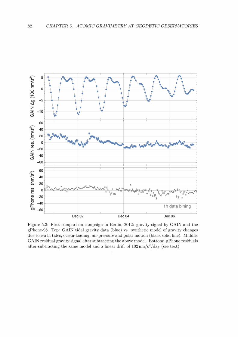
82 CHAPTER 5. ATOMIC GRAVIMETRY AT GEODETIC OBSERVATORIES
--(
/)
---
(/)
---
(/)
Figure 5.3: First comparison campaign in Berlin, 2012: gravity signal by GAIN and thegPhone-98. Top: GAIN tidal gravity data (blue) vs. synthetic model of gravity changesdue to earth tides, ocean-loading, air-pressure and polar motion (black solid line). Middle:GAIN residual gravity signal after subtracting the above model. Bottom: gPhone residualsafter subtracting the same model and a linear drift of 102 nm/s2/day (see text)
.

5.2. MOBILE CAMPAIGNS 83
--(
/)
---
(/)
----
(/)
Figure 5.4: Second comparison campaign in Berlin, 2013: GAIN and the FG5X-220 gravitydata comparison. Top: GAIN data (blue) vs. a synthetic model of gravity changes dueto earth tides, air-pressure and polar motion (black solid line). Middle: GAIN residualgravity signal after subtracting the above model. Bottom: FG5X-220 residual gravityafter subtracting the same model
.
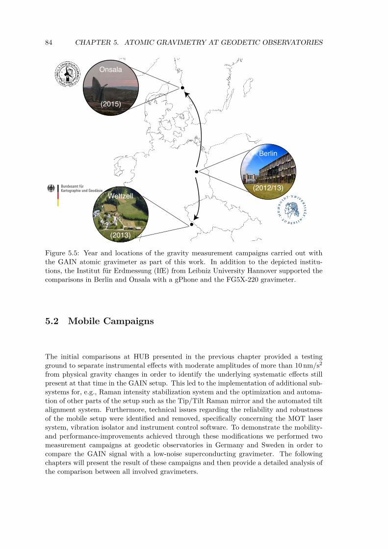
84 CHAPTER 5. ATOMIC GRAVIMETRY AT GEODETIC OBSERVATORIES
Berlin
(2012/13)Wettzell
(2013)
Onsala
(2015)
Figure 5.5: Year and locations of the gravity measurement campaigns carried out withthe GAIN atomic gravimeter as part of this work. In addition to the depicted institu-tions, the Institut für Erdmessung (IfE) from Leibniz University Hannover supported thecomparisons in Berlin and Onsala with a gPhone and the FG5X-220 gravimeter.
5.2 Mobile Campaigns
The initial comparisons at HUB presented in the previous chapter provided a testingground to separate instrumental effects with moderate amplitudes of more than 10 nm/s2
from physical gravity changes in order to identify the underlying systematic effects stillpresent at that time in the GAIN setup. This led to the implementation of additional sub-systems for, e.g., Raman intensity stabilization system and the optimization and automa-tion of other parts of the setup such as the Tip/Tilt Raman mirror and the automated tiltalignment system. Furthermore, technical issues regarding the reliability and robustnessof the mobile setup were identified and removed, specifically concerning the MOT lasersystem, vibration isolator and instrument control software. To demonstrate the mobility-and performance-improvements achieved through these modifications we performed twomeasurement campaigns at geodetic observatories in Germany and Sweden in order tocompare the GAIN signal with a low-noise superconducting gravimeter. The followingchapters will present the result of these campaigns and then provide a detailed analysis ofthe comparison between all involved gravimeters.
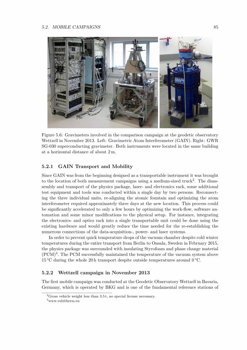
5.2. MOBILE CAMPAIGNS 85
Figure 5.6: Gravimeters involved in the comparison campaign at the geodetic observatoryWettzell in November 2013. Left: Gravimetric Atom Interferometer (GAIN). Right: GWRSG-030 superconducting gravimeter. Both instruments were located in the same buildingat a horizontal distance of about 2 m.
5.2.1 GAIN Transport and MobilitySince GAIN was from the beginning designed as a transportable instrument it was broughtto the location of both measurement campaigns using a medium-sized truck2. The disas-sembly and transport of the physics package, laser- and electronics rack, some additionaltest equipment and tools was conducted within a single day by two persons. Reconnect-ing the three individual units, re-aligning the atomic fountain and optimizing the atominterferometer required approximately three days at the new location. This process couldbe significantly accelerated to only a few hours by optimizing the work-flow, software au-tomation and some minor modifications to the physical setup. For instance, integratingthe electronics- and optics rack into a single transportable unit could be done using theexisting hardware and would greatly reduce the time needed for the re-establishing thenumerous connections of the data-acquisition-, power- and laser systems.
In order to prevent quick temperature drops of the vacuum chamber despite cold wintertemperatures during the entire transport from Berlin to Onsala, Sweden in February 2015,the physics package was surrounded with insulating Styrofoam and phase change material(PCM)3. The PCM successfully maintained the temperature of the vacuum system above15 °C during the whole 20 h transport despite outside temperatures around 0 °C.
5.2.2 Wettzell campaign in November 2013The first mobile campaign was conducted at the Geodetic Observatory Wettzell in Bavaria,Germany, which is operated by BKG and is one of the fundamental reference stations of
2Gross vehicle weight less than 3.5 t, no special license necessary.3www.rubitherm.eu
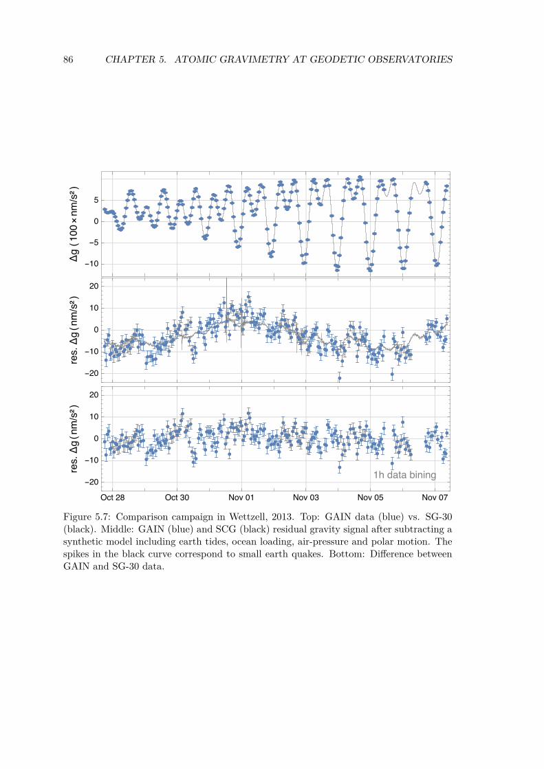
86 CHAPTER 5. ATOMIC GRAVIMETRY AT GEODETIC OBSERVATORIES
--(
×/)
--
(/)
--
(/)
Figure 5.7: Comparison campaign in Wettzell, 2013. Top: GAIN data (blue) vs. SG-30(black). Middle: GAIN (blue) and SCG (black) residual gravity signal after subtracting asynthetic model including earth tides, ocean loading, air-pressure and polar motion. Thespikes in the black curve correspond to small earth quakes. Bottom: Difference betweenGAIN and SG-30 data.
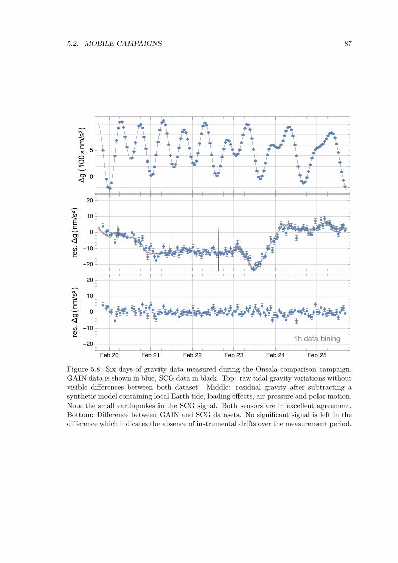
5.2. MOBILE CAMPAIGNS 87
(×
/)
--
(/)
--
(/)
Figure 5.8: Six days of gravity data measured during the Onsala comparison campaign.GAIN data is shown in blue, SCG data in black. Top: raw tidal gravity variations withoutvisible differences between both dataset. Middle: residual gravity after subtracting asynthetic model containing local Earth tide, loading effects, air-pressure and polar motion.Note the small earthquakes in the SCG signal. Both sensors are in excellent agreement.Bottom: Difference between GAIN and SCG datasets. No significant signal is left in thedifference which indicates the absence of instrumental drifts over the measurement period.
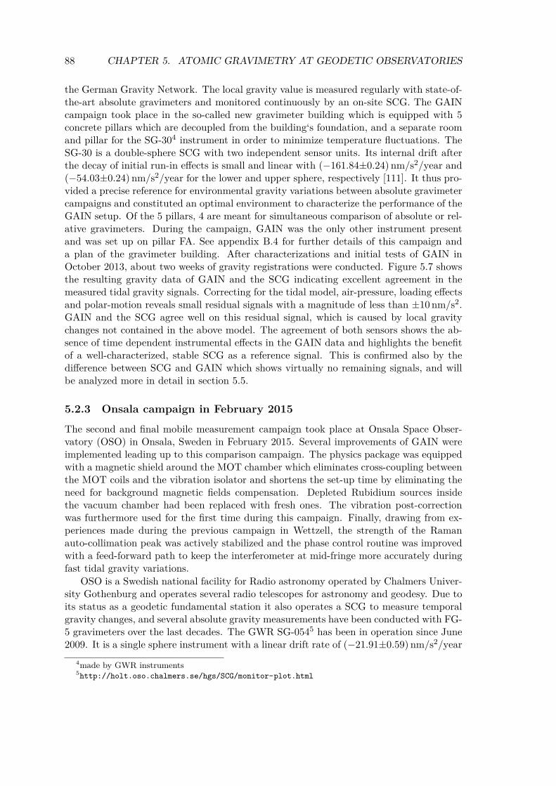
88 CHAPTER 5. ATOMIC GRAVIMETRY AT GEODETIC OBSERVATORIES
the German Gravity Network. The local gravity value is measured regularly with state-of-the-art absolute gravimeters and monitored continuously by an on-site SCG. The GAINcampaign took place in the so-called new gravimeter building which is equipped with 5concrete pillars which are decoupled from the building‘s foundation, and a separate roomand pillar for the SG-304 instrument in order to minimize temperature fluctuations. TheSG-30 is a double-sphere SCG with two independent sensor units. Its internal drift afterthe decay of initial run-in effects is small and linear with (−161.84±0.24) nm/s2/year and(−54.03±0.24) nm/s2/year for the lower and upper sphere, respectively [111]. It thus pro-vided a precise reference for environmental gravity variations between absolute gravimetercampaigns and constituted an optimal environment to characterize the performance of theGAIN setup. Of the 5 pillars, 4 are meant for simultaneous comparison of absolute or rel-ative gravimeters. During the campaign, GAIN was the only other instrument presentand was set up on pillar FA. See appendix B.4 for further details of this campaign anda plan of the gravimeter building. After characterizations and initial tests of GAIN inOctober 2013, about two weeks of gravity registrations were conducted. Figure 5.7 showsthe resulting gravity data of GAIN and the SCG indicating excellent agreement in themeasured tidal gravity signals. Correcting for the tidal model, air-pressure, loading effectsand polar-motion reveals small residual signals with a magnitude of less than ±10 nm/s2.GAIN and the SCG agree well on this residual signal, which is caused by local gravitychanges not contained in the above model. The agreement of both sensors shows the ab-sence of time dependent instrumental effects in the GAIN data and highlights the benefitof a well-characterized, stable SCG as a reference signal. This is confirmed also by thedifference between SCG and GAIN which shows virtually no remaining signals, and willbe analyzed more in detail in section 5.5.
5.2.3 Onsala campaign in February 2015The second and final mobile measurement campaign took place at Onsala Space Obser-vatory (OSO) in Onsala, Sweden in February 2015. Several improvements of GAIN wereimplemented leading up to this comparison campaign. The physics package was equippedwith a magnetic shield around the MOT chamber which eliminates cross-coupling betweenthe MOT coils and the vibration isolator and shortens the set-up time by eliminating theneed for background magnetic fields compensation. Depleted Rubidium sources insidethe vacuum chamber had been replaced with fresh ones. The vibration post-correctionwas furthermore used for the first time during this campaign. Finally, drawing from ex-periences made during the previous campaign in Wettzell, the strength of the Ramanauto-collimation peak was actively stabilized and the phase control routine was improvedwith a feed-forward path to keep the interferometer at mid-fringe more accurately duringfast tidal gravity variations.
OSO is a Swedish national facility for Radio astronomy operated by Chalmers Univer-sity Gothenburg and operates several radio telescopes for astronomy and geodesy. Due toits status as a geodetic fundamental station it also operates a SCG to measure temporalgravity changes, and several absolute gravity measurements have been conducted with FG-5 gravimeters over the last decades. The GWR SG-0545 has been in operation since June2009. It is a single sphere instrument with a linear drift rate of (−21.91±0.59) nm/s2/year
4made by GWR instruments5http://holt.oso.chalmers.se/hgs/SCG/monitor-plot.html
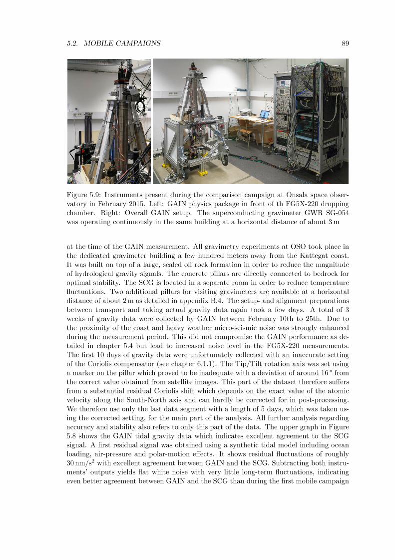
5.2. MOBILE CAMPAIGNS 89
Figure 5.9: Instruments present during the comparison campaign at Onsala space obser-vatory in February 2015. Left: GAIN physics package in front of th FG5X-220 droppingchamber. Right: Overall GAIN setup. The superconducting gravimeter GWR SG-054was operating continuously in the same building at a horizontal distance of about 3 m
at the time of the GAIN measurement. All gravimetry experiments at OSO took place inthe dedicated gravimeter building a few hundred meters away from the Kattegat coast.It was built on top of a large, sealed off rock formation in order to reduce the magnitudeof hydrological gravity signals. The concrete pillars are directly connected to bedrock foroptimal stability. The SCG is located in a separate room in order to reduce temperaturefluctuations. Two additional pillars for visiting gravimeters are available at a horizontaldistance of about 2 m as detailed in appendix B.4. The setup- and alignment preparationsbetween transport and taking actual gravity data again took a few days. A total of 3weeks of gravity data were collected by GAIN between February 10th to 25th. Due tothe proximity of the coast and heavy weather micro-seismic noise was strongly enhancedduring the measurement period. This did not compromise the GAIN performance as de-tailed in chapter 5.4 but lead to increased noise level in the FG5X-220 measurements.The first 10 days of gravity data were unfortunately collected with an inaccurate settingof the Coriolis compensator (see chapter 6.1.1). The Tip/Tilt rotation axis was set usinga marker on the pillar which proved to be inadequate with a deviation of around 16 ° fromthe correct value obtained from satellite images. This part of the dataset therefore suffersfrom a substantial residual Coriolis shift which depends on the exact value of the atomicvelocity along the South-North axis and can hardly be corrected for in post-processing.We therefore use only the last data segment with a length of 5 days, which was taken us-ing the corrected setting, for the main part of the analysis. All further analysis regardingaccuracy and stability also refers to only this part of the data. The upper graph in Figure5.8 shows the GAIN tidal gravity data which indicates excellent agreement to the SCGsignal. A first residual signal was obtained using a synthetic tidal model including oceanloading, air-pressure and polar-motion effects. It shows residual fluctuations of roughly30 nm/s2 with excellent agreement between GAIN and the SCG. Subtracting both instru-ments’ outputs yields flat white noise with very little long-term fluctuations, indicatingeven better agreement between GAIN and the SCG than during the first mobile campaign
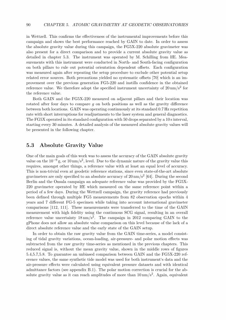
90 CHAPTER 5. ATOMIC GRAVIMETRY AT GEODETIC OBSERVATORIES
in Wettzell. This confirms the effectiveness of the instrumental improvements before thiscampaign and shows the best performance reached by GAIN to date. In order to assessthe absolute gravity value during this campaign, the FG5X-220 absolute gravimeter wasalso present for a direct comparison and to provide a current absolute gravity value asdetailed in chapter 5.3. The instrument was operated by M. Schilling from IfE. Mea-surements with this instrument were conducted in North- and South-facing configurationon both pillars to rule out potential orientation dependent offsets. Each configurationwas measured again after repeating the setup procedure to exclude other potential setuprelated error sources. Both precautions yielded no systematic offsets [70] which is an im-provement over the previous generation FG5-220 and instills confidence in the obtainedreference value. We therefore adopt the specified instrument uncertainty of 20 nm/s2 forthe reference value.
Both GAIN and the FG5X-220 measured on adjacent pillars and their location wasrotated after four days to compare g on both positions as well as the gravity differencebetween both locations. GAIN was operating continuously at its standard 0.7 Hz repetitionrate with short interruptions for readjustments to the laser system and general diagnostics.The FG5X operated in its standard configuration with 50 drops separated by a 10 s interval,starting every 30 minutes. A detailed analysis of the measured absolute gravity values willbe presented in the following chapter.
5.3 Absolute Gravity Value
One of the main goals of this work was to assess the accuracy of the GAIN absolute gravityvalue on the 10−9 g, or 10 nm/s2, level. Due to the dynamic nature of the gravity value thisrequires, amongst other things, a reference value with at least an equal level of accuracy.This is non-trivial even at geodetic reference stations, since even state-of-the-art absolutegravimeters are only specified to an absolute accuracy of 20 nm/s2 [64]. During the secondBerlin and the Onsala campaign an adequate reference value was provided by the FG5X-220 gravimeter operated by IfE which measured on the same reference point within aperiod of a few days. During the Wettzell campaign, the gravity reference had previouslybeen defined through multiple FG5 measurements from 82 observation epochs within 4years and 7 different FG-5 specimen while taking into account international gravimetercomparisons [112, 111]. These measurements were transferred to the time of the GAINmeasurement with high fidelity using the continuous SCG signal, resulting in an overallreference value uncertainty 18 nm/s2. The campaign in 2012 comparing GAIN to thegPhone does not allow an absolute value comparison on this level because of the lack of adirect absolute reference value and the early state of the GAIN setup.
In order to obtain the raw gravity value from the GAIN time-series, a model consist-ing of tidal gravity variations, ocean-loading, air-pressure- and polar motion effects wassubtracted from the raw gravity time-series as mentioned in the previous chapters. Thisreduced signal is, without the mean gravity value, shown in the middle rows of figures5.4,5.7,5.8. To guarantee an unbiased comparison between GAIN and the FG5X-220 ref-erence values, the same synthetic tide model was used for both instrument‘s data and theair-pressure effects were calculated using equivalent pressure datasets and with identicaladmittance factors (see appendix B.1). The polar motion correction is crucial for the ab-solute gravity value as it can reach amplitudes of more than 10 nm/s2. Again, equivalent
5.3. ABSOLUTE GRAVITY VALUE 91
Offset Systematic Error Budgets[nm/s2] Onsala 2015 Wettzell 2013 Berlin 2013Raman Wavefronts 28 ± 22 28 ± 22 28 ± 22RF Group delays 0 ± 10 0 ± 10 0 ± 10Coriolis Effect 12 ± 7 0 ± 15 0 ± 15Raman Frequency Offset 0 ± 7 0 ± 7 0 ± 7Self Gravitation -19 ± 5 -19 ± 5 -19 ± 5Rb Vapor Index -5 ± 5 -5 ± 5 -5 ± 5Quad. Zeeman Shift 0 ± 5 0 ± 5 0 ± 5Light Shift (1-photon) 0 ± 5 0 ± 5 0 ± 20Light Shift (2-photon) 0 ± 5 0 ± 5 0 ± 5Synchronous Vibrations 0 ± 5 -92 ± 50 -92 ± 50Reference Laser Freq. 13 ± 2 10 ± 5 0 ± 20RF Reference Offset. 0 ± 1 0 ± 1 0 ± 40Total Offset 29 ± 29 -78 ± 59 -88 ± 77
Table 5.1: Improvement of the systematic error budget between the three absolutegravimeter comparisons. Each value is given as offset ± uncertainty. The respectivetotal offset was added to the raw GAIN results to obtain the corrected gravity values. Alluncertainties are given as 1σ standard errors (68 % confidence level)
pole coordinates were used for the reduction of both instrument‘s data. A detailed listingof all relevant model parameters for all four campaigns is given in appendix B.
The GAIN raw gravity value obtained from the model reduction was further correctedfor the known systematic effects discussed in chapter 6 by adding the total offset from thesystematic error budgets shown in table 5.1. Due to improvements of the GAIN setup theerror budget was significantly reduced both in the size of the remaining offset and in theassociated uncertainty between the first and the last campaign. To summarize the mainimprovements, the uncertainty was decreased between the Berlin and Wettzell campaignby implementing active Raman intensity stabilization, verifying the reference laser fre-quency using cold atom spectroscopy in the atomic fountain and phase-locking the GAIN10 MHz reference oscillator to a low phase-noise Maser provided by the Wettzell observa-tory. Another significant improvement of the systematic error budget between Wettzelland Onsala was achieved by eliminating synchronous vibrations with the magnetic shieldaround the MOT region and by characterizing the remaining Coriolis effect uncertaintyas detailed in chapter 6.1.1.
The corrected gravity value is valid at the effective measurement height of GAIN whichin generally differs from the height level of the reference value. Both thus have to be trans-ferred to a common height level while accounting for the correct vertical gravity gradientwhich was measured on all relevant reference points using relative gravimeters prior to thecampaigns. The height levels used for the comparison were 1.2 m for the Berlin and Onsalacampaign (the standard setting for FG5X gravimeters), and 1.25 m for the Wettzell cam-paign. The effective measurement height of the GAIN sensor was around 1.38 m and 1.42 mabove ground during the Berlin/Wettzell and Onsala6 campaigns, respectively, as detailed
6The 4 cm increase for Onsala is due to setup changes, namely the MOT magnetic shield after which

92 CHAPTER 5. ATOMIC GRAVIMETRY AT GEODETIC OBSERVATORIES
Absolute Gravity [nm/s2]Onsala 2015 Wettzell 2013 Berlin 2013
GAIN Raw Value 9 817 158 325 ± 1 9 808 369 359 ± 1 9 812 641 207 ± 2Systematic Offset 29 ± 29 -78 ± 59 -88 ± 77Height Offset 729 ± 12 436 ± 10 412 ± 11GAIN corrected 9 817 159 083 ± 31 9 808 369 717 ± 60 9 812 641 532 ± 66Reference value 9 817 159 023 ± 20 9 808 369 633 ± 18 9 812 641 438 ± 23∆gSCG -3 ± 1 -10 ± 1 0 ± 0GAIN-(Ref.+∆gSCG) 63 ± 37 94 ± 63 93 ± 81
Table 5.2: Result of three absolute gravity comparison campaigns in Germany and Sweden,showing good agreement between GAIN and reference gravity values. GAIN raw valuesare obtained from the mean residual, after subtracting earth tides, air-pressure effects andpolar motion. ∆gSCG is an offset from superconducting gravimeter residuals to correct forunmodeled environmental gravity changes between the reference- and GAIN observationperiods (see text). Improvements in the GAIN setup lead to increasing agreement andsubstantially lower uncertainty between the first and last campaign. All uncertainties aregiven as 1σ standard errors (68 % confidence level).
for each campaign in appendix B. These values were obtained by measuring the heightof the detection beam relative to the ground with a tape measure. The atom’s heightwith respect to the floor during the first Raman pulse can then be extracted from thesequence data and inserted into equation 2.37 to obtain the effective measurement height.We estimate the uncertainty of the detection height measurement to 3 mm, mainly dueto difficult access and the lack of precision measuring tools. This dominates the overallheight transfer uncertainty due to the large vertical gradient to approximately 10 nm/s2.
Small environmental gravity variations between observation periods which are notcontained in the synthetic model can still influence the absolute gravity comparison onthis level. During the campaigns in Wettzell and Onsala these variations were accountedfor by transferring the measured gravity values between the different observation periodsusing the SCG signal. This was done by subtracting the SCG residuals’ mean during bothabsolute gravimeter observation periods from each other, yielding:
∆gSCG := gresscg(tgain))− gresscg(t
ref )) (5.1)
where the bar indicates the mean value. ∆gSCG was then subtracted from the respectivereference value. Note that due to the well-characterized, linear drift and low noise of theSCG, this correction can be performed over long time periods with very low uncertaintyand be used to connect several absolute gravity campaigns which was done during theWettzell campaign [112]. Since FG5X-220 and GAIN observations on pillar AC duringthe Onsala campaign were only separated by a few days, this respective correction issmaller and almost negligible in comparison to other effects. The same is presumably truefor the absolute gravity campaign in Berlin, however no SCG signal was available on siteduring this comparison.
the physics package had to be raised

5.4. SHORT-TERM STABILITY AND NOISE 93
The final differences between the gravity values of GAIN and the respective references,including all of the above corrections, are summarized in table 5.2. GAIN and the referencevalues agree on a 95 % or 2σ confidence interval, with the best agreement during the lastcampaign in Onsala with a gravity value difference of only (63±37) nm/s2. This representsan improvement of almost a factor two with respect to the Wettzell campaign and is crucialfor applications of atomic gravimeters in geodesy where long-term, secular signals of a few10 nm/s2 are of interest.
This level of accuracy represents the current state-of-the-art in absolute gravimetrywhich has, to the knowledge the author, only been demonstrated by very few other atomicgravimeters and is consistent with comparisons of several FG5 specimen [65, 113]. Thefirst two campaigns show a slightly larger difference between GAIN and the referencevalue, which is consistent with the larger systematic uncertainties due to (at the time ofthe campaign) outstanding instrumental improvements of GAIN. It is noteworthy thatduring all three campaigns the GAIN result is higher than the reference values obtainedby FG5 measurements, which agrees with the results of other atomic gravimeters [65, 11]and could indicate hidden systematic effects in either of the involved instruments. Futurestudies of all relevant systematic error budgets and comparisons to a third, independentabsolute gravimeter implementation would therefore be of high interest to identify thelocation and source of this difference. The results shown in table 5.2 for the Onsala andWettzell campaign differ slightly from the results published in [14], caused by a number ofcorrections implemented during the improved analysis during this work. For the Wettzellcampaign, an inaccurate vertical gradient had been used before which was replaced withthe recommended, published value for this location [114]. For the Onsala campaign anal-ysis, the GAIN raw value increased by around 12 nm/s2 after accounting for the correctpolar motion correction. A small additional offset caused by the Coriolis effect listed intable 5.1 was also added here. While both alterations increased the difference betweenGAIN and the FG5 reference values, the qualitative result of close agreement betweenboth instruments remains.
The overall uncertainty is dominated by the GAIN and FG5 systematic error budgetsas shown in table 5.2. Further improvement on this side is therefore necessary and should,on the GAIN side, be focused on reducing Raman wavefront aberration effects. In order toraise the confidence in the achieved level of accuracy and compare the GAIN sensor to manyinstruments at once, participation at an international or European absolute gravimetercomparison (ICAG, ECAG) seem like the natural next step. In order to accelerate theidentification and study of systematics in GAIN on the low 10−9 g level, improving theshort-term sensitivity is very beneficial to shorten the required averaging times. Thecurrent status and sources of measurements noise will therefore be detailed in the followingchapter.
5.4 Short-Term Stability and Noise
The residual GAIN gravity signal after correcting for tidal and other environmental effectsis dominated by largely uncorrelated short-term fluctuations due to measurement noise.The total observed noise is a mixture of several contributions, the most important of whichwere isolated and quantified as described below. The root mean square (RMS) values ofshot-to-shot fluctuations were divided by the square root of the instrumental repetition
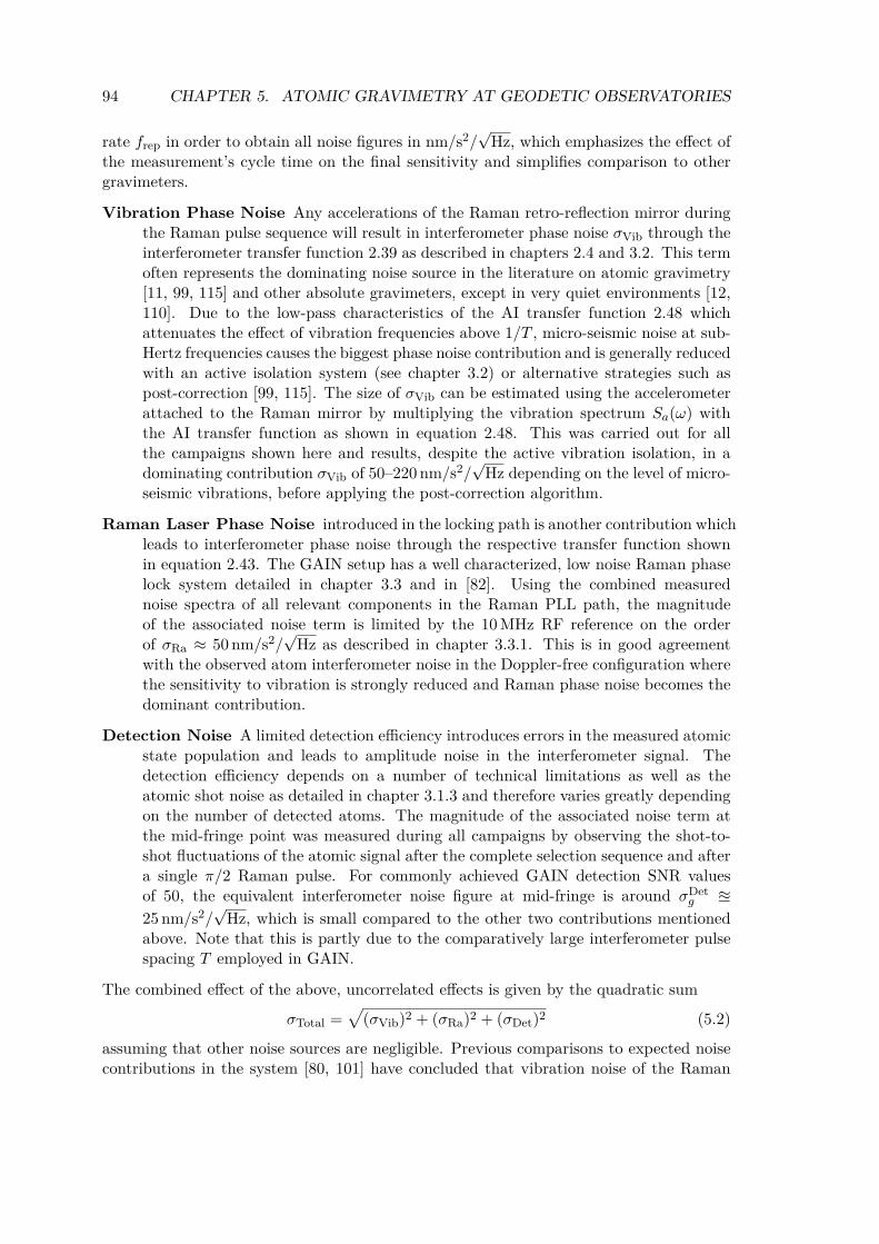
94 CHAPTER 5. ATOMIC GRAVIMETRY AT GEODETIC OBSERVATORIES
rate frep in order to obtain all noise figures in nm/s2/√
Hz, which emphasizes the effect ofthe measurement’s cycle time on the final sensitivity and simplifies comparison to othergravimeters.
Vibration Phase Noise Any accelerations of the Raman retro-reflection mirror duringthe Raman pulse sequence will result in interferometer phase noise σVib through theinterferometer transfer function 2.39 as described in chapters 2.4 and 3.2. This termoften represents the dominating noise source in the literature on atomic gravimetry[11, 99, 115] and other absolute gravimeters, except in very quiet environments [12,110]. Due to the low-pass characteristics of the AI transfer function 2.48 whichattenuates the effect of vibration frequencies above 1/T , micro-seismic noise at sub-Hertz frequencies causes the biggest phase noise contribution and is generally reducedwith an active isolation system (see chapter 3.2) or alternative strategies such aspost-correction [99, 115]. The size of σVib can be estimated using the accelerometerattached to the Raman mirror by multiplying the vibration spectrum Sa(ω) withthe AI transfer function as shown in equation 2.48. This was carried out for allthe campaigns shown here and results, despite the active vibration isolation, in adominating contribution σVib of 50–220 nm/s2/
√Hz depending on the level of micro-
seismic vibrations, before applying the post-correction algorithm.
Raman Laser Phase Noise introduced in the locking path is another contribution whichleads to interferometer phase noise through the respective transfer function shownin equation 2.43. The GAIN setup has a well characterized, low noise Raman phaselock system detailed in chapter 3.3 and in [82]. Using the combined measurednoise spectra of all relevant components in the Raman PLL path, the magnitudeof the associated noise term is limited by the 10 MHz RF reference on the orderof σRa ≈ 50 nm/s2/
√Hz as described in chapter 3.3.1. This is in good agreement
with the observed atom interferometer noise in the Doppler-free configuration wherethe sensitivity to vibration is strongly reduced and Raman phase noise becomes thedominant contribution.
Detection Noise A limited detection efficiency introduces errors in the measured atomicstate population and leads to amplitude noise in the interferometer signal. Thedetection efficiency depends on a number of technical limitations as well as theatomic shot noise as detailed in chapter 3.1.3 and therefore varies greatly dependingon the number of detected atoms. The magnitude of the associated noise term atthe mid-fringe point was measured during all campaigns by observing the shot-to-shot fluctuations of the atomic signal after the complete selection sequence and aftera single π/2 Raman pulse. For commonly achieved GAIN detection SNR valuesof 50, the equivalent interferometer noise figure at mid-fringe is around σDet
g ≊25 nm/s2/
√Hz, which is small compared to the other two contributions mentioned
above. Note that this is partly due to the comparatively large interferometer pulsespacing T employed in GAIN.
The combined effect of the above, uncorrelated effects is given by the quadratic sum
σTotal =√(σVib)2 + (σRa)2 + (σDet)2 (5.2)
assuming that other noise sources are negligible. Previous comparisons to expected noisecontributions in the system [80, 101] have concluded that vibration noise of the Raman

5.4. SHORT-TERM STABILITY AND NOISE 95
mirror dominates overall. Due to an incorrect pre-factor of√2π in the vibration phase
noise computation carried out in [80], however, σVib was actually overestimated by arounda factor 2 before. Figures 5.10 to 5.13 show the observed measurement noise during allfour presented campaigns with and without applied post-correction as well as the vibrationinduced gravity noise computed from the mirror accelerometer in a time-resolved manner.The spectrograms in figures 5.10, 5.11 clearly show the much higher vibration noise above1 Hz frequency at the university building in Berlin with lots of human activity and acommon concrete floor, compared to the data measured on decoupled concrete pillars at theremote geodetic observatories shown in figures 5.12,5.13. In the micro-seismic band from0.1–1 Hz there is no fundamental difference between both situations, seasonal and weatherchanges seem to be of more importance here. Micro-seismic noise was actually lowestduring the Berlin 2012 campaigns, somewhat stronger during the Berlin and Wettzellmeasurements in 2013 and by far the strongest in Onsala 2015 due to the proximity ofthe coastline and winter storms. Below 1 Hz the spectrograms of both observatory datasets show plenty of earthquakes, which are obscured in the Berlin data by human activity(steps) next to the seismometer. The AI vibration phase noise indicated by the yellow linesin figures 5.10-5.13 correlates very well with noise in the micro-seismic band as expecteddue to the low-pass filtering behavior of the interferometer transfer function 2.48. In orderto avoid artifacts due to earthquakes and other strong, low-frequency events, a 10 samplemedian filter was applied to all line plots in figures 5.10-5.13. The quadratic difference
∆GAIN =√(σnoPC
Tot )2 − (σPCTot)
2
of the observed gravity noise with and without applied post-correction shows both inits magnitude and its time dependence excellent agreement with the computed vibrationnoise σVib. This can be expected from equation 5.2 assuming that the post-correctionremoves virtually all of the vibration noise measured by the platform accelerometer. Theagreement thus confirms the accuracy of the vibration phase-noise calculation and theeffectiveness of the post-correction algorithm applied to improve the GAIN gravity signal.The noise contained in the final, post-corrected gravity signal is in fact uncorrelated withvibrations within the bandwidth of the platform accelerometer. According to the abovelist of expected noise sources, the signal after post-correction should thus be limited byRaman Laser phase noise σRa ≈ 50 nm/
√Hz. The observed levels are, however, between
62–260 nm/s2/√
Hz which is up to 5 times larger during the measurement campaigns asshown by the solid blue line in figures 5.10 to 5.13. The known noise sources alone cantherefore not fully account for the observed gravity noise. A strong variation during thefirst three campaigns indicate that additional environmental effects dominate, however, noclear correlation with such influences was found. Some potential noise sources requiringfurther investigation are
• Acoustic vibration’s outside the accelerometer‘s bandwidth, which could be reducedin the future through an acoustic isolation curtain or box.
• Air convection and related refractive index changes between the Raman mirror andthe vacuum window. The GAIN physics package was only covered with a simplewooden box and insulating bubble wrap foil to suppress air movement in this region.This should in the future be improved through tubing around the Raman free-airbeam path.

96 CHAPTER 5. ATOMIC GRAVIMETRY AT GEODETIC OBSERVATORIES
(
)/
()
/
Δ//
/
( ) ( )Δ σ (calculated)
//
-150 -140 -130 -120 -110 -100Figure 5.10: Spectrograms of vertical acceleration on the GAIN isolation platform (top)and on the ground (middle) during the gPhone comparison in Berlin in 2012, showingan intermediate micro-seismic activity and very high noise levels above 1 Hz due to dailyhuman activity and the 2nd floor physics lab environment. Bottom: Time-dependenceof observed GAIN sensitivity. The blue lines show the gravity residual RMS value over10 min data segments with and without post-correction (PC). The yellow lines show twoestimates of the expected vibration noise before PC as detailed below. Strongly time-dependent excess noise clearly exists and compromises the overall sensitivity above theRaman Laser Phase noise limit (gray dashed line). See text for further discussion.

5.4. SHORT-TERM STABILITY AND NOISE 97
(
)/
()
/
Δ//
/
( ) ( )Δ σ (calculated)
//
-150 -140 -130 -120 -110 -100Figure 5.11: Spectrograms of vertical acceleration on the GAIN isolation platform (top)and on the ground (middle) during the comparison to the FG5X-220 in Berlin 2013.Clearly visible is a weak micro-seismic background and high noise level above 1 Hz dueto human activity, particularly during the day. Bottom: Time-dependence of observedGAIN sensitivity. The blue lines show the gravity residual RMS value over 10 min datasegments with and without post-correction (PC). The yellow lines show two estimates ofthe expected vibration noise before PC as detailed below. A time-dependent excess noisesource clearly compromises the overall GAIN noise level above the Raman Laser Phasenoise limit (gray dashed line). See text for further discussion.
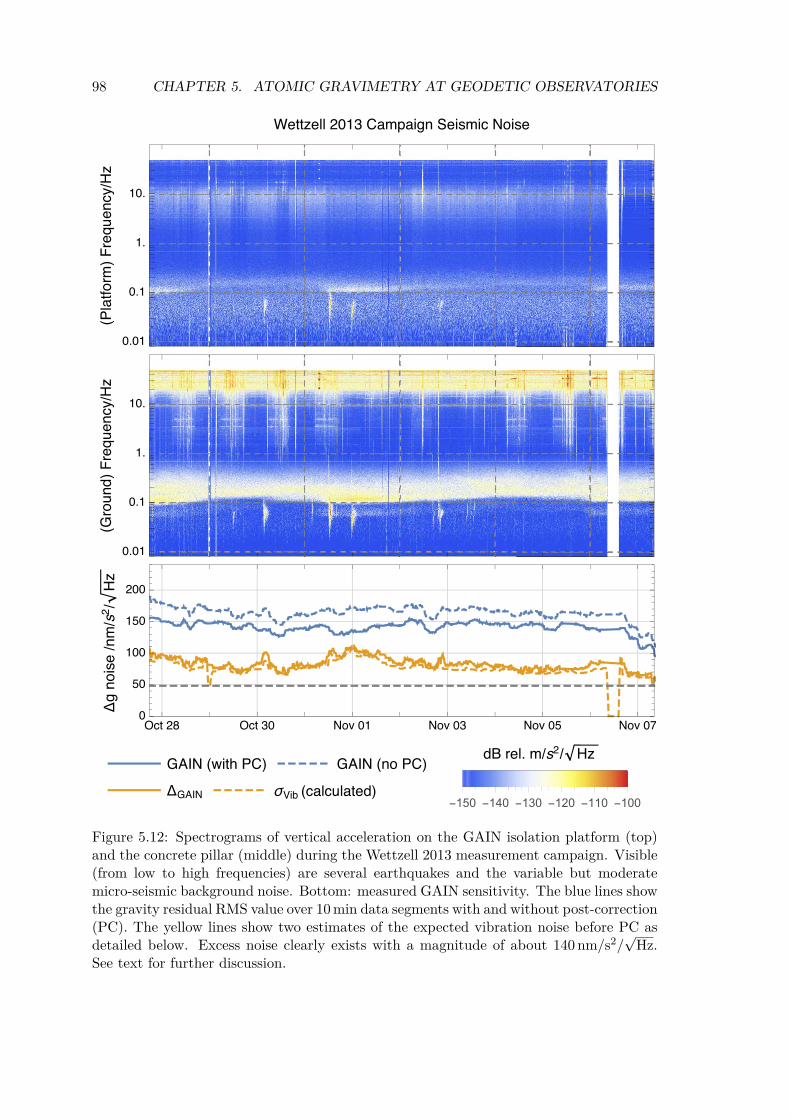
98 CHAPTER 5. ATOMIC GRAVIMETRY AT GEODETIC OBSERVATORIES
(
)/
()
/
Δ//
/
( ) ( )Δ σ (calculated)
//
-150 -140 -130 -120 -110 -100Figure 5.12: Spectrograms of vertical acceleration on the GAIN isolation platform (top)and the concrete pillar (middle) during the Wettzell 2013 measurement campaign. Visible(from low to high frequencies) are several earthquakes and the variable but moderatemicro-seismic background noise. Bottom: measured GAIN sensitivity. The blue lines showthe gravity residual RMS value over 10 min data segments with and without post-correction(PC). The yellow lines show two estimates of the expected vibration noise before PC asdetailed below. Excess noise clearly exists with a magnitude of about 140 nm/s2/
√Hz.
See text for further discussion.
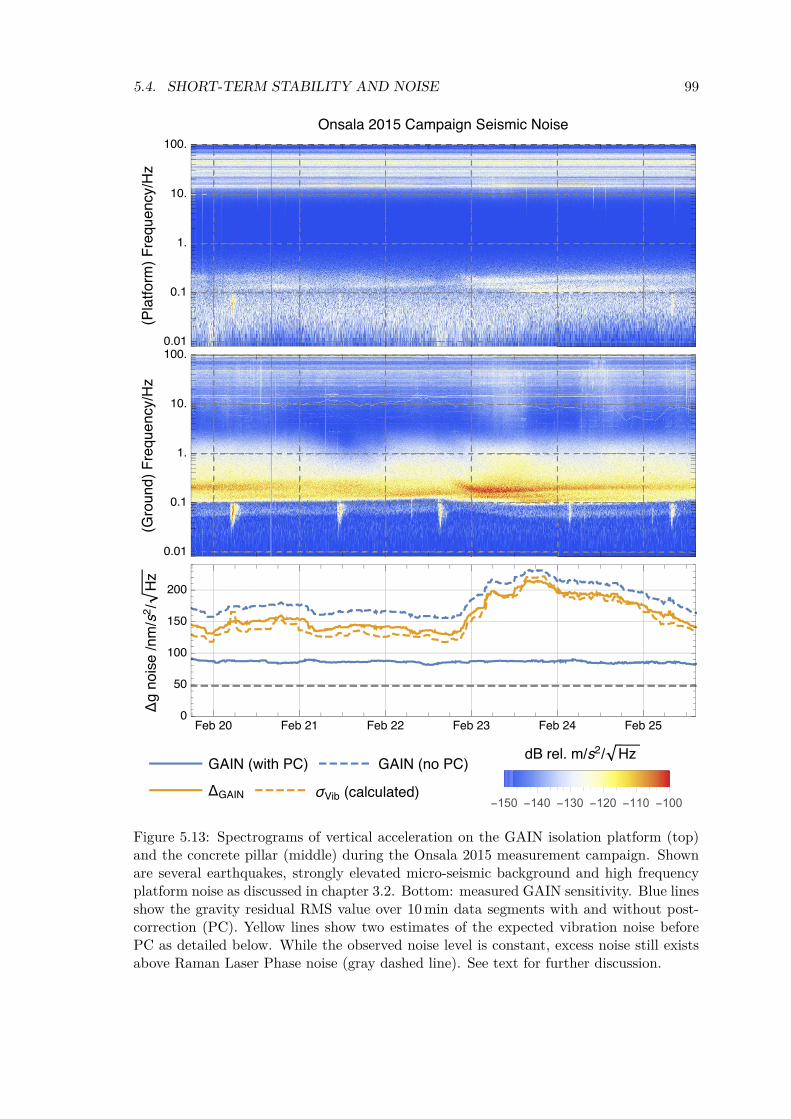
5.4. SHORT-TERM STABILITY AND NOISE 99
(
)/
()
/
Δ//
/
( ) ( )Δ σ (calculated)
//
-150 -140 -130 -120 -110 -100Figure 5.13: Spectrograms of vertical acceleration on the GAIN isolation platform (top)and the concrete pillar (middle) during the Onsala 2015 measurement campaign. Shownare several earthquakes, strongly elevated micro-seismic background and high frequencyplatform noise as discussed in chapter 3.2. Bottom: measured GAIN sensitivity. Blue linesshow the gravity residual RMS value over 10 min data segments with and without post-correction (PC). Yellow lines show two estimates of the expected vibration noise beforePC as detailed below. While the observed noise level is constant, excess noise still existsabove Raman Laser Phase noise (gray dashed line). See text for further discussion.
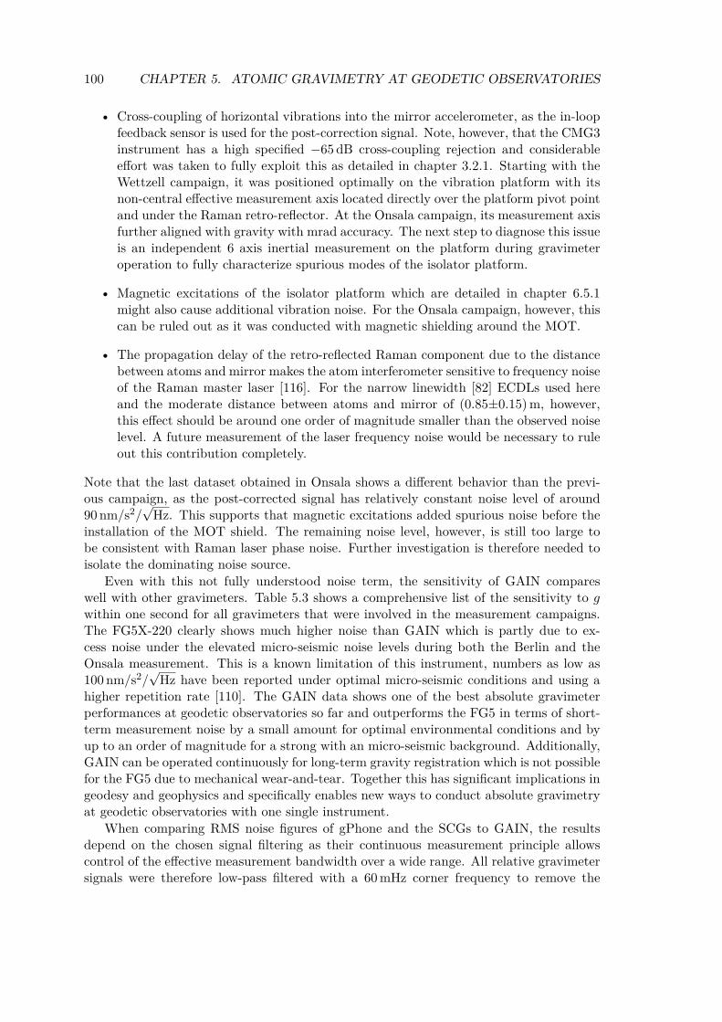
100 CHAPTER 5. ATOMIC GRAVIMETRY AT GEODETIC OBSERVATORIES
• Cross-coupling of horizontal vibrations into the mirror accelerometer, as the in-loopfeedback sensor is used for the post-correction signal. Note, however, that the CMG3instrument has a high specified −65 dB cross-coupling rejection and considerableeffort was taken to fully exploit this as detailed in chapter 3.2.1. Starting with theWettzell campaign, it was positioned optimally on the vibration platform with itsnon-central effective measurement axis located directly over the platform pivot pointand under the Raman retro-reflector. At the Onsala campaign, its measurement axisfurther aligned with gravity with mrad accuracy. The next step to diagnose this issueis an independent 6 axis inertial measurement on the platform during gravimeteroperation to fully characterize spurious modes of the isolator platform.
• Magnetic excitations of the isolator platform which are detailed in chapter 6.5.1might also cause additional vibration noise. For the Onsala campaign, however, thiscan be ruled out as it was conducted with magnetic shielding around the MOT.
• The propagation delay of the retro-reflected Raman component due to the distancebetween atoms and mirror makes the atom interferometer sensitive to frequency noiseof the Raman master laser [116]. For the narrow linewidth [82] ECDLs used hereand the moderate distance between atoms and mirror of (0.85±0.15)m, however,this effect should be around one order of magnitude smaller than the observed noiselevel. A future measurement of the laser frequency noise would be necessary to ruleout this contribution completely.
Note that the last dataset obtained in Onsala shows a different behavior than the previ-ous campaign, as the post-corrected signal has relatively constant noise level of around90 nm/s2/
√Hz. This supports that magnetic excitations added spurious noise before the
installation of the MOT shield. The remaining noise level, however, is still too large tobe consistent with Raman laser phase noise. Further investigation is therefore needed toisolate the dominating noise source.
Even with this not fully understood noise term, the sensitivity of GAIN compareswell with other gravimeters. Table 5.3 shows a comprehensive list of the sensitivity to gwithin one second for all gravimeters that were involved in the measurement campaigns.The FG5X-220 clearly shows much higher noise than GAIN which is partly due to ex-cess noise under the elevated micro-seismic noise levels during both the Berlin and theOnsala measurement. This is a known limitation of this instrument, numbers as low as100 nm/s2/
√Hz have been reported under optimal micro-seismic conditions and using a
higher repetition rate [110]. The GAIN data shows one of the best absolute gravimeterperformances at geodetic observatories so far and outperforms the FG5 in terms of short-term measurement noise by a small amount for optimal environmental conditions and byup to an order of magnitude for a strong with an micro-seismic background. Additionally,GAIN can be operated continuously for long-term gravity registration which is not possiblefor the FG5 due to mechanical wear-and-tear. Together this has significant implications ingeodesy and geophysics and specifically enables new ways to conduct absolute gravimetryat geodetic observatories with one single instrument.
When comparing RMS noise figures of gPhone and the SCGs to GAIN, the resultsdepend on the chosen signal filtering as their continuous measurement principle allowscontrol of the effective measurement bandwidth over a wide range. All relative gravimetersignals were therefore low-pass filtered with a 60 mHz corner frequency to remove the
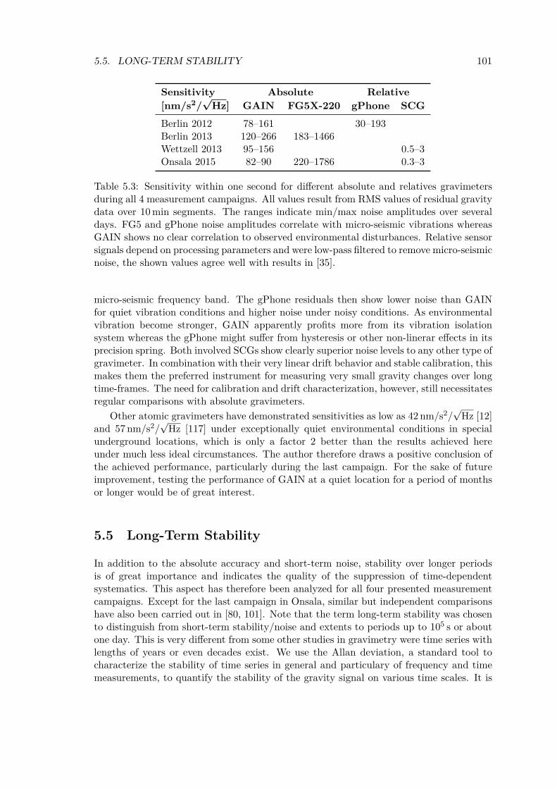
5.5. LONG-TERM STABILITY 101
Sensitivity Absolute Relative[nm/s2/
√Hz] GAIN FG5X-220 gPhone SCG
Berlin 2012 78–161 30–193Berlin 2013 120–266 183–1466Wettzell 2013 95–156 0.5–3Onsala 2015 82–90 220–1786 0.3–3
Table 5.3: Sensitivity within one second for different absolute and relatives gravimetersduring all 4 measurement campaigns. All values result from RMS values of residual gravitydata over 10 min segments. The ranges indicate min/max noise amplitudes over severaldays. FG5 and gPhone noise amplitudes correlate with micro-seismic vibrations whereasGAIN shows no clear correlation to observed environmental disturbances. Relative sensorsignals depend on processing parameters and were low-pass filtered to remove micro-seismicnoise, the shown values agree well with results in [35].
micro-seismic frequency band. The gPhone residuals then show lower noise than GAINfor quiet vibration conditions and higher noise under noisy conditions. As environmentalvibration become stronger, GAIN apparently profits more from its vibration isolationsystem whereas the gPhone might suffer from hysteresis or other non-linerar effects in itsprecision spring. Both involved SCGs show clearly superior noise levels to any other type ofgravimeter. In combination with their very linear drift behavior and stable calibration, thismakes them the preferred instrument for measuring very small gravity changes over longtime-frames. The need for calibration and drift characterization, however, still necessitatesregular comparisons with absolute gravimeters.
Other atomic gravimeters have demonstrated sensitivities as low as 42 nm/s2/√
Hz [12]and 57 nm/s2/
√Hz [117] under exceptionally quiet environmental conditions in special
underground locations, which is only a factor 2 better than the results achieved hereunder much less ideal circumstances. The author therefore draws a positive conclusion ofthe achieved performance, particularly during the last campaign. For the sake of futureimprovement, testing the performance of GAIN at a quiet location for a period of monthsor longer would be of great interest.
5.5 Long-Term Stability
In addition to the absolute accuracy and short-term noise, stability over longer periodsis of great importance and indicates the quality of the suppression of time-dependentsystematics. This aspect has therefore been analyzed for all four presented measurementcampaigns. Except for the last campaign in Onsala, similar but independent comparisonshave also been carried out in [80, 101]. Note that the term long-term stability was chosento distinguish from short-term stability/noise and extents to periods up to 105 s or aboutone day. This is very different from some other studies in gravimetry were time series withlengths of years or even decades exist. We use the Allan deviation, a standard tool tocharacterize the stability of time series in general and particulary of frequency and timemeasurements, to quantify the stability of the gravity signal on various time scales. It is
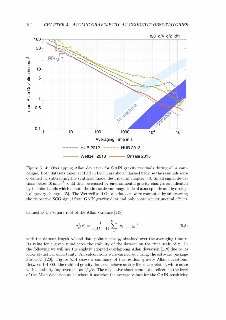
102 CHAPTER 5. ATOMIC GRAVIMETRY AT GEODETIC OBSERVATORIES
///// 90/
Figure 5.14: Overlapping Allan deviation for GAIN gravity residuals during all 4 cam-paigns. Both datasets taken at HUB in Berlin are shown dashed because the residuals wereobtained by subtracting the synthetic model described in chapter 5.3. Small signal devia-tions below 10 nm/s2 could thus be caused by environmental gravity changes as indicatedby the blue bands which denote the timescale and magnitude of atmospheric and hydrolog-ical gravity changes [35]. The Wettzell and Onsala datasets were computed by subtractingthe respective SCG signal from GAIN gravity data and only contain instrumental effects.
defined as the square root of the Allan variance [118]
σ2y(τ) =
1
2 (M − 1)
M−1∑i=1
[yi+1 − yi]2 (5.3)
with the dataset length M and data point means yi obtained over the averaging time τ .Its value for a given τ indicates the stability of the dataset on the time scale of τ . Inthe following we will use the slightly adopted overlapping Allan deviation [119] due to itslower statistical uncertainty. All calculations were carried out using the software packageStable32 [120]. Figure 5.14 shows a summary of the residual gravity Allan deviations.Between 1–1000 s the residual gravity datasets behave mostly like uncorrelated, white noisewith a stability improvement as 1/
√τ . The respective short-term noise reflects in the level
of the Allan deviation at 1 s where it matches the average values for the GAIN sensitivity

5.5. LONG-TERM STABILITY 103
shown in table 5.3. Beyond 1000 s the behavior differs between campaigns and shows theprogress made by the successive instrumental improvements. Note that the two dashedlines are potentially compromised by actual environmental gravity changes as a syntheticmodel was subtracted as detailed in chapter 5.3. The exact size of instrumental drift istherefore hard to extract from those datasets. This is not the case for the Wettzell andOnsala datasets were simultaneous SCG signals were subtracted from the GAIN gravitysignal. Updated SCG calibration factors from chapter 5.5.1 were used for this purpose andno additional time-delay was applied. The Wettzell dataset shows residual instabilities ontimescales of 3×10³–105 s after which it falls to a minimum value of 0.6 nm/s2. Beyond105 s instabilities become apparent due to long-term drifts which lead to an increasingAllan deviation. This is mostly consistent with the analysis presented in [80, 101] withthe exception that no long-term drift beyond 105 s was reported there. This is presumabledue to the linear drift reduction carried out in that analysis.
The Onsala dataset shows clearly the best GAIN performance achieved so far, withthe lowest short-term noise of around 90 nm/s2/
√Hz averaging down consistently until
3×10⁴ s. Flicker noise on semi-diurnal time scales then leads to a constant Allan deviationon the 0.5–0.6 nm/s2 level which decreases again at diurnal periods and reaches its lowestvalue of 0.4 nm/s2 just beyond 105 s. This is, to the knowledge of the author, the bestreported stability for an atomic gravimeter so far and has been detailed in a separatepublication [14]. Absolute gravimeter stabilities of below 1 nm/s2 have, in fact, to ourknowledge not been published for any other absolute gravimeter so far.
5.5.1 Scale Factor DeterminationAll relative gravimeters need to be calibrated to obtain the scale factor b such that themeasured output voltage signals x can be related to physical gravity differences through∆g = b · x. For superconducting gravimeters b is usually measured through simultaneousmeasurements of absolute gravimeters such as the FG5 and utilizes the time-dependence oftidal gravity variations. A scale factor estimate can be extracted from a linear regressionof the SCG data points xi and the absolute gravimeter observations yi through thefollowing formula [121]
b =
∑(xi − x) (yi − y)∑
(xi − x)2σ2b =
1
n
∑(yi − a− bxi
)∑
(xi − x)2(5.4)
with the offset a = y − bx. Here, symbols with a hat denote estimated values and barsindicate the arithmetic mean. The uncertainty of the resulting estimates depends mostlyon absolute gravimeter noise and the size of tidal gravity variations. This method thereforeworks best if the amplitude of those variations are at their monthly maximum.
The simultaneous gravity registrations of GAIN during the Wettzell and Onsala cam-paigns provided not only an ideal scenario to characterize the performance of GAIN butalso to estimate the scale factor of the two involved SCG gravimeters and compare itsvalue and uncertainty to previous calibration campaigns. Table 5.4 shows the summary ofobtained SCG scale factors during the GAIN Wettzell and Onsala campaigns compared toprevious estimates obtained from many FG5 measurements performed over several years.The estimated values of both methods agree within their error bars, however, the relativeuncertainties reached with the GAIN data are much better with 0.3 ‰ and 0.4 ‰ during

104 CHAPTER 5. ATOMIC GRAVIMETRY AT GEODETIC OBSERVATORIES
Scale Factor Calibration Wettzell SG30 Onsala SG054[nm/s2/V] bottom topFG5 campaigns (mean) −739.0±1.0 −678.4±1.0 −774.3±3.0GAIN campaign −740.25±0.23 −680.30±0.21 −773.91±0.31
Table 5.4: Comparison of SCG scale factor regressions using GAIN and previously obtainedFG5 gravity data, yielding strongly reduced uncertainty. The GAIN datasets are shownin figures 5.7, 5.8 and have a length of 10 and 6 days for Wettzell and Onsala, respectively.The slightly increased uncertainty in Onsala, despite the reduced measurement noise, isdue to the smaller earth tide amplitude and the shorter dataset. Uncertainties given as1σ standard errors.
the Wettzell and Onsala campaign, respectively. This is 3-5 times better than the previousFG5 results [121] even though those represent an average over multiple campaigns overa longer period of time. Even under optimal micro-seismic noise conditions, optimizedmeasurement schedules and when measuring only during the maximal tide amplitudes,the expected uncertainty of FG5 calibration campaigns would be 0.5 nm/s2 after 6 daysand only reaches 0.2 nm/s2 after 60 days of registration [122].
GAIN therefore provides a quicker and significantly more precise way to determineSCG scale factors due to its high repetition rate, continuous operation and low noiseunder noisy environmental conditions, which is of considerable benefit in geodesy andgeophysics.
5.5.2 Time Delay
When comparing the output signal of atomic- and superconducting gravimeters, the differ-ent transfer functions and the associated signal distortions have to be taken into account.Low frequency group/phase delays are particularly problematic as they subject earth tides,by far the largest gravitational effect in the above datasets, to an effective time delay.
The transfer function of SCGs is mostly determined by the analog low-pass filter,data acquisition hardware and internal feedback integrator [123]. For the two instrumentsin Wettzell and Onsala, which both have an analog anti-aliasing filter with a corner-frequency of around 60 s, the total time delay was measured to be on the order of 10 sas shown in table 5.5. Atom interferometers, on the other hand, effectively measurethe atom‘s acceleration relative to the retro-reflection mirror during the interferometerpulse sequence. Their transfer function is therefore determined primarily by the vibrationisolation system. For the GAIN active vibration isolator presented in chapter 3.2, thisresults in significant group delays only around the effective resonance frequency of theclosed-loop system around 50 mHz. As shown in figure 3.9 the group delay essentiallyvanishes above and below this resonance. No observable lag should therefore be presentin the GAIN gravity data, however, a significant time delay of 20 s relative to the SCG attidal frequencies was estimated from the GAIN Wettzell data in [80]. The underlying causefor this discrepancy could not be proven conclusively and has therefore been investigatedfurther in this work.
The analysis carried out in [80] is based on the maximization of the cross-correlationcoefficient Rxy(τ) between GAIN and SCG signals [124]. While this is a reliable and
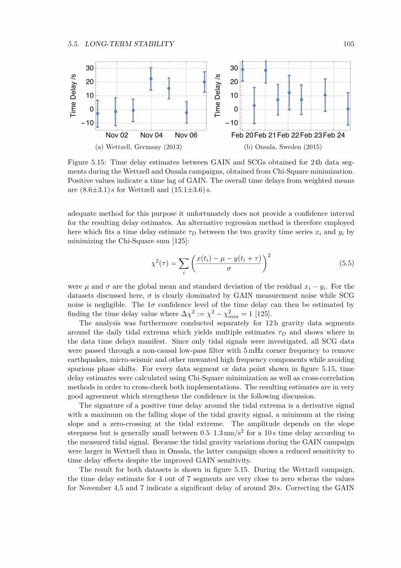
5.5. LONG-TERM STABILITY 105
-
/
(a) Wettzell, Germany (2013)
-
/
(b) Onsala, Sweden (2015)
Figure 5.15: Time delay estimates between GAIN and SCGs obtained for 24h data seg-ments during the Wettzell and Onsala campaigns, obtained from Chi-Square minimization.Positive values indicate a time lag of GAIN. The overall time delays from weighted meansare (8.6±3.1) s for Wettzell and (15.1±3.6) s.
adequate method for this purpose it unfortunately does not provide a confidence intervalfor the resulting delay estimates. An alternative regression method is therefore employedhere which fits a time delay estimate τD between the two gravity time series xi and yi byminimizing the Chi-Square sum [125]:
χ2(τ) =∑i
(x(ti)− µ− y(ti + τ)
σ
)2
(5.5)
were µ and σ are the global mean and standard deviation of the residual xi − yi. For thedatasets discussed here, σ is clearly dominated by GAIN measurement noise while SCGnoise is negligible. The 1σ confidence level of the time delay can then be estimated byfinding the time delay value where ∆χ2 := χ2 − χ2
min = 1 [125].The analysis was furthermore conducted separately for 12 h gravity data segments
around the daily tidal extrema which yields multiple estimates τD and shows where inthe data time delays manifest. Since only tidal signals were investigated, all SCG datawere passed through a non-causal low-pass filter with 5 mHz corner frequency to removeearthquakes, micro-seismic and other unwanted high frequency components while avoidingspurious phase shifts. For every data segment or data point shown in figure 5.15, timedelay estimates were calculated using Chi-Square minimization as well as cross-correlationmethods in order to cross-check both implementations. The resulting estimates are in verygood agreement which strengthens the confidence in the following discussion.
The signature of a positive time delay around the tidal extrema is a derivative signalwith a maximum on the falling slope of the tidal gravity signal, a minimum at the risingslope and a zero-crossing at the tidal extreme. The amplitude depends on the slopesteepness but is generally small between 0.5–1.3 nm/s2 for a 10 s time delay according tothe measured tidal signal. Because the tidal gravity variations during the GAIN campaignwere larger in Wettzell than in Onsala, the latter campaign shows a reduced sensitivity totime delay effects despite the improved GAIN sensitivity.
The result for both datasets is shown in figure 5.15. During the Wettzell campaign,the time delay estimate for 4 out of 7 segments are very close to zero wheras the valuesfor November 4,5 and 7 indicate a significant delay of around 20 s. Correcting the GAIN
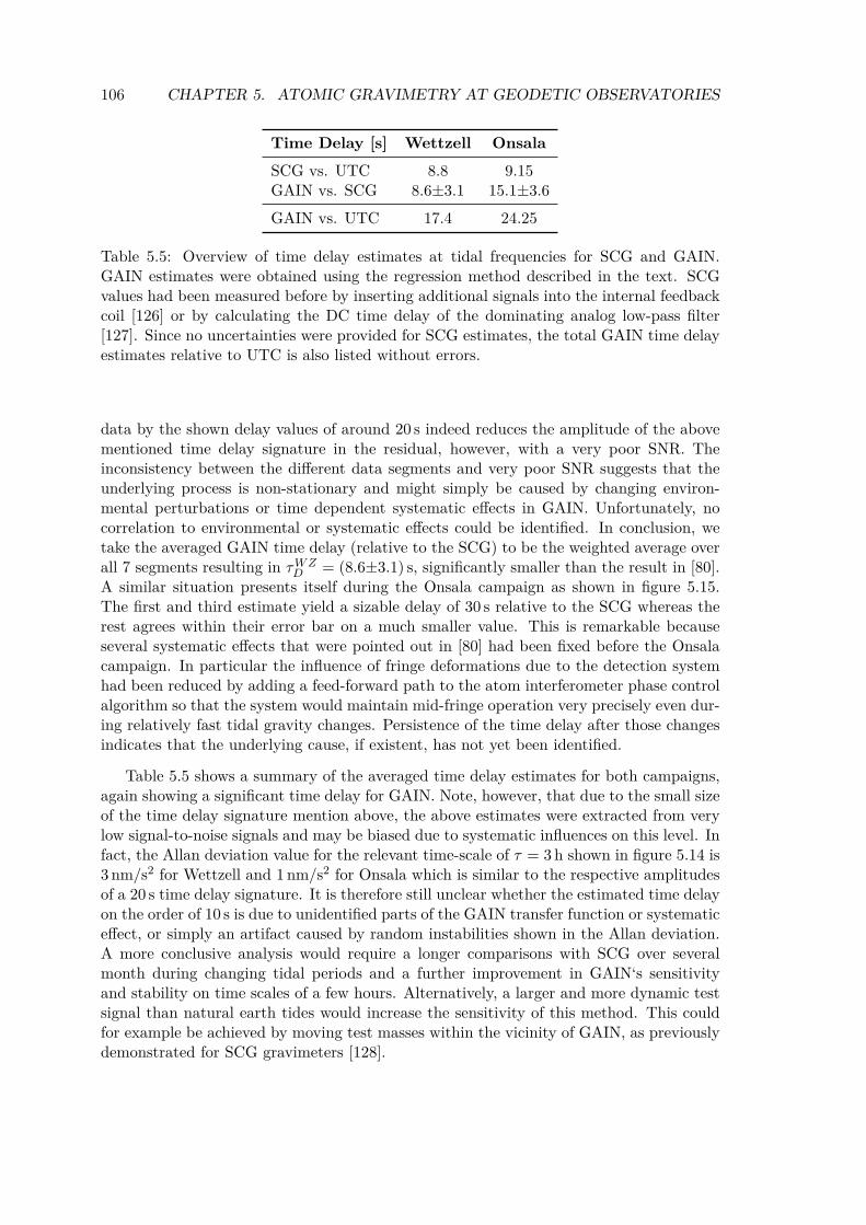
106 CHAPTER 5. ATOMIC GRAVIMETRY AT GEODETIC OBSERVATORIES
Time Delay [s] Wettzell OnsalaSCG vs. UTC 8.8 9.15GAIN vs. SCG 8.6±3.1 15.1±3.6GAIN vs. UTC 17.4 24.25
Table 5.5: Overview of time delay estimates at tidal frequencies for SCG and GAIN.GAIN estimates were obtained using the regression method described in the text. SCGvalues had been measured before by inserting additional signals into the internal feedbackcoil [126] or by calculating the DC time delay of the dominating analog low-pass filter[127]. Since no uncertainties were provided for SCG estimates, the total GAIN time delayestimates relative to UTC is also listed without errors.
data by the shown delay values of around 20 s indeed reduces the amplitude of the abovementioned time delay signature in the residual, however, with a very poor SNR. Theinconsistency between the different data segments and very poor SNR suggests that theunderlying process is non-stationary and might simply be caused by changing environ-mental perturbations or time dependent systematic effects in GAIN. Unfortunately, nocorrelation to environmental or systematic effects could be identified. In conclusion, wetake the averaged GAIN time delay (relative to the SCG) to be the weighted average overall 7 segments resulting in τWZ
D = (8.6±3.1) s, significantly smaller than the result in [80].A similar situation presents itself during the Onsala campaign as shown in figure 5.15.The first and third estimate yield a sizable delay of 30 s relative to the SCG whereas therest agrees within their error bar on a much smaller value. This is remarkable becauseseveral systematic effects that were pointed out in [80] had been fixed before the Onsalacampaign. In particular the influence of fringe deformations due to the detection systemhad been reduced by adding a feed-forward path to the atom interferometer phase controlalgorithm so that the system would maintain mid-fringe operation very precisely even dur-ing relatively fast tidal gravity changes. Persistence of the time delay after those changesindicates that the underlying cause, if existent, has not yet been identified.
Table 5.5 shows a summary of the averaged time delay estimates for both campaigns,again showing a significant time delay for GAIN. Note, however, that due to the small sizeof the time delay signature mention above, the above estimates were extracted from verylow signal-to-noise signals and may be biased due to systematic influences on this level. Infact, the Allan deviation value for the relevant time-scale of τ = 3 h shown in figure 5.14 is3 nm/s2 for Wettzell and 1 nm/s2 for Onsala which is similar to the respective amplitudesof a 20 s time delay signature. It is therefore still unclear whether the estimated time delayon the order of 10 s is due to unidentified parts of the GAIN transfer function or systematiceffect, or simply an artifact caused by random instabilities shown in the Allan deviation.A more conclusive analysis would require a longer comparisons with SCG over severalmonth during changing tidal periods and a further improvement in GAIN‘s sensitivityand stability on time scales of a few hours. Alternatively, a larger and more dynamic testsignal than natural earth tides would increase the sensitivity of this method. This couldfor example be achieved by moving test masses within the vicinity of GAIN, as previouslydemonstrated for SCG gravimeters [128].
5.5. LONG-TERM STABILITY 107
SummaryThis chapter presented all main results of four gravity measurement campaigns whichcompared the atom interferometer GAIN to a gPhone spring gravimeter, two supercon-ducting instruments and the FG5X-220 absolute gravimeter. The later two measurementcampaigns were conducted at geodetic observatories in Wettzell, Germany and OnsalaSweden and demonstrate the mobility and robustness of the GAIN setup.
The measured sensitivity, long-term stability and accuracy of GAIN competes excep-tionally well with current state-of-the-art gravimeters. The shown combination of long-term gravity monitoring with high stability, absolute accuracy and mobility was foundto be unique to atomic gravimeters such as GAIN. Resulting application in geodesy andgeophysics, such as the calibration of superconducting gravimeters were presented anddiscussed.
In order to deliver the stability and accuracy presented here, a range systematic effectswere analysed and removed from the measurement, which will be detailed in the nextchapter.

108 CHAPTER 5. ATOMIC GRAVIMETRY AT GEODETIC OBSERVATORIES

Chapter 6
Systematics
The main goal of this thesis is to exploit the potential of atom interferometers for appli-cations in geodesy and geophysics. The absolute accuracy and stability of the measuredgravity value is of fundamental importance for these tasks. The understanding and controlof systematic effects is therefore of great importance for the development and applicationof atomic gravimeters. As a part of this work a thorough analysis of expected and observedsystematics in GAIN was conducted before, during and after the implementation of thepreviously discussed instrumental improvements. The result is presented in the followingchapter for each investigated shift.
In contrast to precision measurements of fundamental physical constants or test of thelaws of physics, gravity measurements on Earth are subject to a variety of environmentalinfluences such as tidal forces or local mass redistributions discussed in detail in chapter1. This complicates the identification of systematic effects as a large background of realgravity signals first has to be removed before instrumental effects become visible. Be-cause synthetic models for the prediction of tidal and other effects are limited to levelsof approximately 10 nm/s2, the comparison to superconducting gravimeters as a reliable,low-noise reference during both mobile comparison campaigns turned out to be essentialfor this task. The present analysis for the GAIN setup was influenced by, but not limitedto, those presented on similar experiments in [27, 83]. Whenever possible, the analysiswas performed using the atomic signal in the atomic fountain itself instead of externalreference signals or simulations. This enables in-situ checking of the experimental pa-rameters, in some cases even within a measurement campaign, and makes the instrumentindependent of external calibrations and references and marks another advantage of atominterferometers compared to other types of gravimeters.
Due to the sheer number of relevant systematic effects a categorization into the un-derlying physical sources was attempted. An alternative ordering exists which orders theeffects by their reaction to a flip of the momentum recoil direction keff. As this is ofgreat practical importance for this experiment, a separate sub-chapter 6.7 deals with thecharacteristics of this rejection. Finally, a summary of all regarded systematics will bepresented in table 6.3.
109
110 CHAPTER 6. SYSTEMATICS
6.1 Fundamental EffectsThis sub-chapter deals with fundamental phase shifts arising in the practical experimentthat were not accounted for in the phase shift calculation in chapter 2.3. This encompassesrotations of the laboratory reference frame as well as potential higher-order phase-shiftswhich are listed in [85] and which are too small to play a role. A general relativistic cal-culation of the atom interferometer phase presented in [25, 129] has also been considered.Since the largest additional term in this calculation is smaller than 10−13 g for the GAINexperimental parameters, however, these relativistic effects can safely be neglected here.Note, that the finite speed-of-light also manifests as a phase shift in the relativistic model.Because it can also be derived without a full GR calculation and actually needs to beconsidered for GAIN, it will be treated separately in chapter 6.1.3.
6.1.1 Coriolis or Sagnac Phase ShiftDue to the finite temperature and imperfect vertical alignment of the launch, the atomsin the atomic fountain will exhibit a small, residual horizontal velocity. This results in aspatial area A spanned by the atom interferometer which leads to a rotation dependentphase term due to the Sagnac effect [84]:
∆Φsag =2m
ℏΩ · A =
2m
ℏΩ · (v0 × vrec)T
2 = 2Ω · (v0 × keff) (6.1)
with the atomic velocity vector v0 and the coordinate frame rotation rate Ω. For agravimeter with vertical Raman beams in a laboratory frame subject to Earth‘s rotationrate ΩE = 2π/Tsidereal, this leads to a shift in the measured gravity value of:
∆gCor = 2(ΩE cos θ
)vew = 2ΩEvew (6.2)
where vew is the atomic velocity along the West direction, θ is the geographical latitudeand ΩE the effective rotation rate at a given measurement site which is maximal at theequator and vanishes on the poles. Note that this result can alternatively be derived byinserting the vertical component of the Coriolis acceleration aCor = −2Ω × v into theinterferometer phase formula 2.20, hence the term Coriolis shift which will be used herefrom now on. Also note that vew obviously varies within the atom cloud due to the finitetemperature. The experimentally relevant quantity is the mean horizontal velocity vew ofthe subset of atoms which arrive in the detection zone and contribute to the measuredsignal.
In order to keep the Coriolis shift below 10 nm/s2 in Berlin, Germany with ΩE ≊44.46 µrad/s, the upper limit for vew given by equation 6.2 is 127 µm/s. This would bedifficult to ensure permanently in our current setup due to the spreading of the atomiccloud, much larger size of the detection volume and potential slow drifts of the atomiclaunch vector due to MOT power fluctuations.
One method to isolate ∆gCor from the gravity signal is to rotate the entire apparatusby 180 ° during a measurement which, if all other parameters remain constant, reverses vewand thus the Coriolis shift [130]. We instead employ a method first proposed in [86] whichrotates the Raman laser wave vector keff during the interferometer sequence by tiltingthe retro-reflecting mirror. The Coriolis acceleration can then be strongly suppressed byrotating the Raman beams in the opposite direction of Earth‘s rotation ΩE . Specifically,
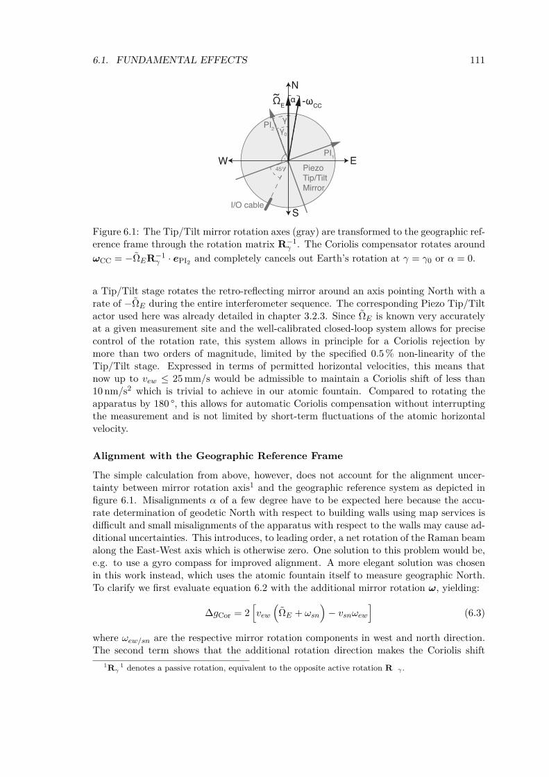
6.1. FUNDAMENTAL EFFECTS 111
PI1
PI2
PiezoTip/TiltMirror
I/O cable
45°
γ
E
N
S
W
ΩE -ωCCα
γ0
~
Figure 6.1: The Tip/Tilt mirror rotation axes (gray) are transformed to the geographic ref-erence frame through the rotation matrix R−1
γ . The Coriolis compensator rotates aroundωCC = −ΩER−1
γ · ePI2 and completely cancels out Earth’s rotation at γ = γ0 or α = 0.
a Tip/Tilt stage rotates the retro-reflecting mirror around an axis pointing North with arate of −ΩE during the entire interferometer sequence. The corresponding Piezo Tip/Tiltactor used here was already detailed in chapter 3.2.3. Since ΩE is known very accuratelyat a given measurement site and the well-calibrated closed-loop system allows for precisecontrol of the rotation rate, this system allows in principle for a Coriolis rejection bymore than two orders of magnitude, limited by the specified 0.5 % non-linearity of theTip/Tilt stage. Expressed in terms of permitted horizontal velocities, this means thatnow up to vew ≤ 25 mm/s would be admissible to maintain a Coriolis shift of less than10 nm/s2 which is trivial to achieve in our atomic fountain. Compared to rotating theapparatus by 180 °, this allows for automatic Coriolis compensation without interruptingthe measurement and is not limited by short-term fluctuations of the atomic horizontalvelocity.
Alignment with the Geographic Reference Frame
The simple calculation from above, however, does not account for the alignment uncer-tainty between mirror rotation axis1 and the geographic reference system as depicted infigure 6.1. Misalignments α of a few degree have to be expected here because the accu-rate determination of geodetic North with respect to building walls using map services isdifficult and small misalignments of the apparatus with respect to the walls may cause ad-ditional uncertainties. This introduces, to leading order, a net rotation of the Raman beamalong the East-West axis which is otherwise zero. One solution to this problem would be,e.g. to use a gyro compass for improved alignment. A more elegant solution was chosenin this work instead, which uses the atomic fountain itself to measure geographic North.To clarify we first evaluate equation 6.2 with the additional mirror rotation ω, yielding:
∆gCor = 2[vew
(ΩE + ωsn
)− vsnωew
](6.3)
where ωew/sn are the respective mirror rotation components in west and north direction.The second term shows that the additional rotation direction makes the Coriolis shift
1R 1γ denotes a passive rotation, equivalent to the opposite active rotation R γ .
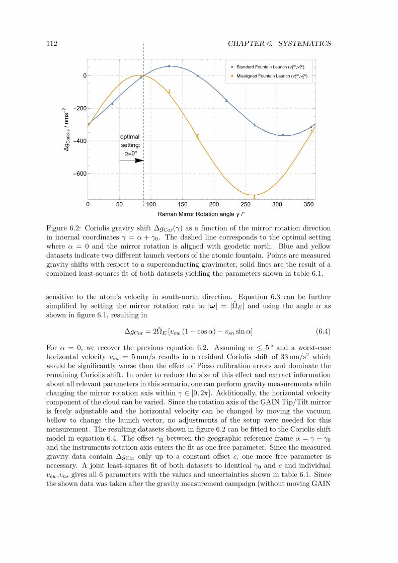
112 CHAPTER 6. SYSTEMATICS
0 50 100 150 200 250 300 350
-600
-400
-200
0
Raman Mirror Rotation angle /°
g Coriolis/nms
-2
optimalsetting:=0°
Standard Fountain Launch (v1ew,v1ns)Misaligned Fountain Launch (v2ew,v2ns)
Figure 6.2: Coriolis gravity shift ∆gCor(γ) as a function of the mirror rotation directionin internal coordinates γ = α + γ0. The dashed line corresponds to the optimal settingwhere α = 0 and the mirror rotation is aligned with geodetic north. Blue and yellowdatasets indicate two different launch vectors of the atomic fountain. Points are measuredgravity shifts with respect to a superconducting gravimeter, solid lines are the result of acombined least-squares fit of both datasets yielding the parameters shown in table 6.1.
sensitive to the atom’s velocity in south-north direction. Equation 6.3 can be furthersimplified by setting the mirror rotation rate to |ω| = |ΩE | and using the angle α asshown in figure 6.1, resulting in
∆gCor = 2ΩE [vew (1− cosα)− vsn sinα] (6.4)
For α = 0, we recover the previous equation 6.2. Assuming α ≤ 5 ° and a worst-casehorizontal velocity vsn = 5 mm/s results in a residual Coriolis shift of 33 nm/s2 whichwould be significantly worse than the effect of Piezo calibration errors and dominate theremaining Coriolis shift. In order to reduce the size of this effect and extract informationabout all relevant parameters in this scenario, one can perform gravity measurements whilechanging the mirror rotation axis within γ ∈ [0, 2π]. Additionally, the horizontal velocitycomponent of the cloud can be varied. Since the rotation axis of the GAIN Tip/Tilt mirroris freely adjustable and the horizontal velocity can be changed by moving the vacuumbellow to change the launch vector, no adjustments of the setup were needed for thismeasurement. The resulting datasets shown in figure 6.2 can be fitted to the Coriolis shiftmodel in equation 6.4. The offset γ0 between the geographic reference frame α = γ − γ0and the instruments rotation axis enters the fit as one free parameter. Since the measuredgravity data contain ∆gCor only up to a constant offset c, one more free parameter isnecessary. A joint least-squares fit of both datasets to identical γ0 and c and individualvew,vns gives all 6 parameters with the values and uncertainties shown in table 6.1. Sincethe shown data was taken after the gravity measurement campaign (without moving GAIN
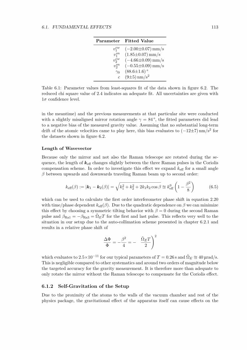
6.1. FUNDAMENTAL EFFECTS 113
Parameter Fitted Valuevew1 (−2.00±0.07)mm/svsn1 (1.85±0.07)mm/svew2 (−4.66±0.09)mm/svsn2 (−0.55±0.09)mm/sγ0 (88.6±1.6) °c (9±5) nm/s2
Table 6.1: Parameter values from least-squares fit of the data shown in figure 6.2. Thereduced chi square value of 2.4 indicates an adequate fit. All uncertainties are given with1σ confidence level.
in the meantime) and the previous measurements at that particular site were conductedwith a slightly misaligned mirror rotation angle γ = 84 °, the fitted parameters did leadto a negative bias of the measured gravity value. Assuming that no substantial long-termdrift of the atomic velocities came to play here, this bias evaluates to (−12±7) nm/s2 forthe datasets shown in figure 6.2.
Length of Wavevector
Because only the mirror and not also the Raman telescope are rotated during the se-quence, the length of keff changes slightly between the three Raman pulses in the Corioliscompensation scheme. In order to investigate this effect we expand keff for a small angleβ between upwards and downwards traveling Raman beam up to second order:
keff(β) := |k1 − k2(β)| =√
k21 + k22 + 2k1k2 cosβ ≊ k0eff
(1− β2
8
)(6.5)
which can be used to calculate the first order interferometer phase shift in equation 2.20with time/phase dependent keff(β). Due to the quadratic dependence on β we can minimizethis effect by choosing a symmetric tilting behavior with β = 0 during the second Ramanpulse and βRa1 = −βRa3 = ΩET for the first and last pulse. This reflects very well to thesituation in our setup due to the auto-collimation scheme presented in chapter 6.2.1 andresults in a relative phase shift of
∆Φ
Φ= −β2
4= −
(ΩET
2
)2
which evaluates to 2.5×10⁻¹¹ for our typical parameters of T = 0.26 s and ΩE ≊ 40 µrad/s.This is negligible compared to other systematics and around two orders of magnitude belowthe targeted accuracy for the gravity measurement. It is therefore more than adequate toonly rotate the mirror without the Raman telescope to compensate for the Coriolis effect.
6.1.2 Self-Gravitation of the SetupDue to the proximity of the atoms to the walls of the vacuum chamber and rest of thephysics package, the gravitational effect of the apparatus itself can cause effects on the
114 CHAPTER 6. SYSTEMATICS
10 nm/s2 level and has to be considered. A detailed FEM simulation of the GAIN self-gravitation was performed in [93], its main result is included here for completeness. It isbased on the original CAD design of the physics package and calculates the Newtoniangravitation exerted by equivalent point masses on the atoms during their free fall. Theresulting interferometer phase shift is derived by computing the perturbed trajectories andcorresponding phase terms during the atom-light interaction during the Raman pulses2.The biggest influence was caused by the magnetic shield of the ion-pump and the solidaluminum block on top of the interferometer zone. All significant components togetheradded up in [93] result in a net gravity bias of 19 nm/s2 for the usual experimental param-eters T = 0.26 s. The high fidelity of the CAD model yields a relatively small uncertaintyof only 0.5 % of this value. Due to the fact that some components of the apparatus, suchas the MOT magnetic shield, were not included in this analysis, we instead assume alarger uncertainty of 5 nm/s2 for this effect. This effect currently does not limit the finalaccuracy of the instrument and can readily be improved with moderate computationalcost by increasing the fidelity of the FEM model as outlined in [93].
6.1.3 Finite Speed of Light
Chirping the Raman frequencies during the interferometer may introduce a spurious phaseshift if only one frequency component is chirped. For a stationary atom, the propagationdelay between laser source and atom would result in an identical chirp centered arounda slightly different frequency and have very little effect. Due to the constant accelerationof the atoms during their free fall, however, the propagation delay changes during theinterferometer sequence which leads to a modified effective chirp-rate and an associatedcorrection of the gravity value [11, 27, 131]
∆gc = 2v0c
α1 + α2
α1 − α2(6.6)
where v0 is the atomic velocity during the π pulse and αi is the chirp-rate of the respectiveRaman frequency component so that α = α1−α2 compensates for the Doppler shift. Thisis closely related to retardation effects caused by the finite speed of light which mustbe corrected in falling corner-cube gravimeters[132]. Note that due to our symmetricsequence with the π pulse close to the apex this effect is quite small in comparison toother configurations which simply drop the atoms. In order to remove it completely weapply frequency chirps to both Raman frequencies α1 = −α2 ≊ ±12.58 MHz/s so that∆gc vanishes. Moreover, the induced gravity bias changes sign when reversing the chirp-rate and will thus be rejected additionally by the k-reversal technique [131]. We thereforeconclude that speed-of-light effects do not contribute significantly to the systematic errorbudget.
6.2 Raman Beam Effects
This section contains all effects which directly influence the wave-vector, wavelength orphase of the Raman beams during the interferometer sequence. keff, or its projection
2An additional path integral component also exists but is too small to be relevant here [93].
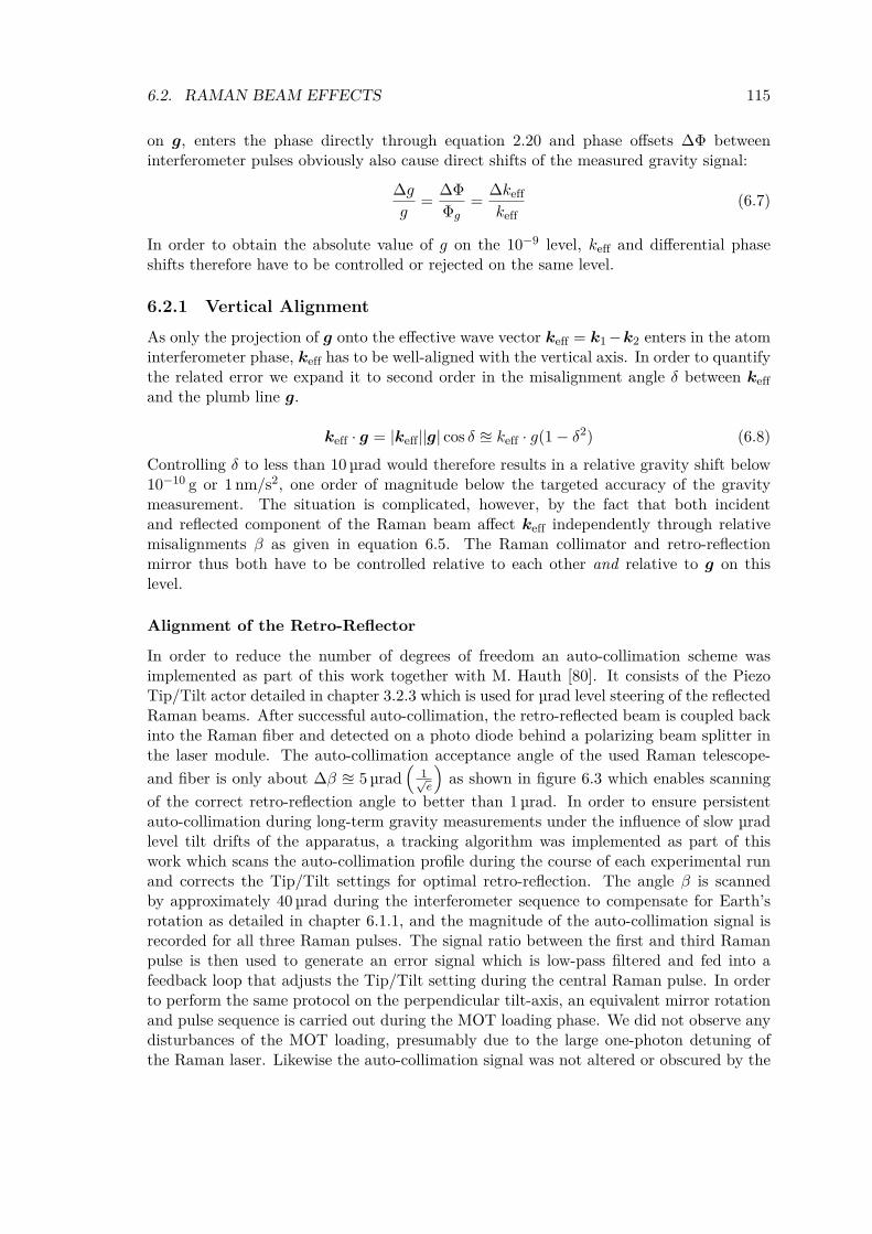
6.2. RAMAN BEAM EFFECTS 115
on g, enters the phase directly through equation 2.20 and phase offsets ∆Φ betweeninterferometer pulses obviously also cause direct shifts of the measured gravity signal:
∆g
g=
∆Φ
Φg=
∆keffkeff
(6.7)
In order to obtain the absolute value of g on the 10−9 level, keff and differential phaseshifts therefore have to be controlled or rejected on the same level.
6.2.1 Vertical AlignmentAs only the projection of g onto the effective wave vector keff = k1−k2 enters in the atominterferometer phase, keff has to be well-aligned with the vertical axis. In order to quantifythe related error we expand it to second order in the misalignment angle δ between keffand the plumb line g.
keff · g = |keff||g| cos δ ≊ keff · g(1− δ2) (6.8)Controlling δ to less than 10 µrad would therefore results in a relative gravity shift below10−10 g or 1 nm/s2, one order of magnitude below the targeted accuracy of the gravitymeasurement. The situation is complicated, however, by the fact that both incidentand reflected component of the Raman beam affect keff independently through relativemisalignments β as given in equation 6.5. The Raman collimator and retro-reflectionmirror thus both have to be controlled relative to each other and relative to g on thislevel.
Alignment of the Retro-Reflector
In order to reduce the number of degrees of freedom an auto-collimation scheme wasimplemented as part of this work together with M. Hauth [80]. It consists of the PiezoTip/Tilt actor detailed in chapter 3.2.3 which is used for µrad level steering of the reflectedRaman beams. After successful auto-collimation, the retro-reflected beam is coupled backinto the Raman fiber and detected on a photo diode behind a polarizing beam splitter inthe laser module. The auto-collimation acceptance angle of the used Raman telescope-and fiber is only about ∆β ≊ 5 µrad
(1√e
)as shown in figure 6.3 which enables scanning
of the correct retro-reflection angle to better than 1 µrad. In order to ensure persistentauto-collimation during long-term gravity measurements under the influence of slow µradlevel tilt drifts of the apparatus, a tracking algorithm was implemented as part of thiswork which scans the auto-collimation profile during the course of each experimental runand corrects the Tip/Tilt settings for optimal retro-reflection. The angle β is scannedby approximately 40 µrad during the interferometer sequence to compensate for Earth’srotation as detailed in chapter 6.1.1, and the magnitude of the auto-collimation signal isrecorded for all three Raman pulses. The signal ratio between the first and third Ramanpulse is then used to generate an error signal which is low-pass filtered and fed into afeedback loop that adjusts the Tip/Tilt setting during the central Raman pulse. In orderto perform the same protocol on the perpendicular tilt-axis, an equivalent mirror rotationand pulse sequence is carried out during the MOT loading phase. We did not observe anydisturbances of the MOT loading, presumably due to the large one-photon detuning ofthe Raman laser. Likewise the auto-collimation signal was not altered or obscured by the
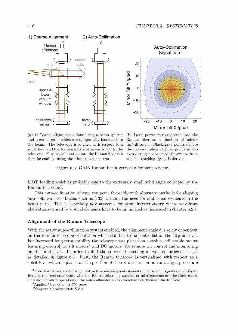
116 CHAPTER 6. SYSTEMATICS
CCD
spirit level /mirror
upper &lower
vacuumwindow
lenscornercube
tip/tiltmirror
Ramantelescope
1) Coarse Alignment 2) Auto-Collimation
(a) 1) Coarse alignment is done using a beam splitterand a corner-cube which are temporarily inserted intothe beam. The telescope is aligned with respect to aspirit level and the Raman mirror afterwards w/r to thetelescope. 2) Auto-collimation into the Raman fiber canthen be enabled using the Piezo tip/tilt mirror.
- ---
/µ/µ
- ( )
(b) Laser power retro-reflected into theRaman fiber as a function of mirrortip/tilt angle. Black/gray points denotethe peak-sampling at three points in twoaxes during in-sequence tilt sweeps fromwhich a tracking signal is derived.
Figure 6.3: GAIN Raman beam vertical alignment scheme.
MOT loading which is probably due to the extremely small solid angle collected by theRaman telescope3.
This auto-collimation scheme competes favorably with alternate methods for aligninganti-collinear laser beams such as [133] without the need for additional elements in thebeam path. This is especially advantageous for atom interferometry where wavefrontaberrations caused by optical elements have to be minimized as discussed in chapter 6.2.4.
Alignment of the Raman Telescope
With the active auto-collimation system enabled, the alignment angle δ is solely dependenton the Raman telescope orientation which still has to be controlled on the 10 µrad level.For increased long-term stability the telescope was placed on a stable, adjustable mountfeaturing electrolytic tilt meters4 and DC motors5 for remote tilt control and monitoringon the µrad level. In order to find the correct tilt setting a two-step process is usedas detailed in figure 6.3. First, the Raman telescope is verticalized with respect to aspirit level which is placed at the position of the retro-reflection mirror using a procedure
3Note that the auto-collimation peak in later measurements showed similar size but significant ellipticity.Because the semi-axes rotate with the Raman telescope, warping or misalignments are the likely cause.This did not affect operation of the auto-collimator and is therefore not discussed further here.
4Applied Geomechanics 755 series5Newport Motorizer 860a S3820
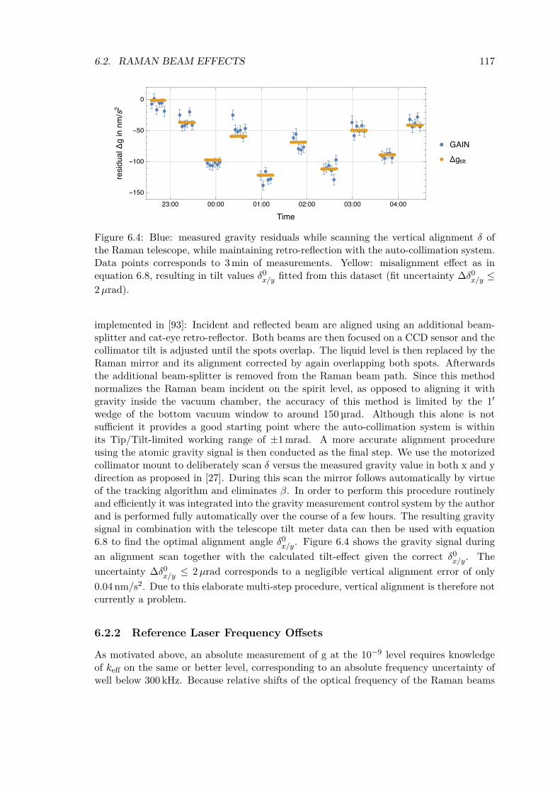
6.2. RAMAN BEAM EFFECTS 117
---
/
Figure 6.4: Blue: measured gravity residuals while scanning the vertical alignment δ ofthe Raman telescope, while maintaining retro-reflection with the auto-collimation system.Data points corresponds to 3 min of measurements. Yellow: misalignment effect as inequation 6.8, resulting in tilt values δ0x/y fitted from this dataset (fit uncertainty ∆δ0x/y ≤2µrad).
implemented in [93]: Incident and reflected beam are aligned using an additional beam-splitter and cat-eye retro-reflector. Both beams are then focused on a CCD sensor and thecollimator tilt is adjusted until the spots overlap. The liquid level is then replaced by theRaman mirror and its alignment corrected by again overlapping both spots. Afterwardsthe additional beam-splitter is removed from the Raman beam path. Since this methodnormalizes the Raman beam incident on the spirit level, as opposed to aligning it withgravity inside the vacuum chamber, the accuracy of this method is limited by the 1′wedge of the bottom vacuum window to around 150 µrad. Although this alone is notsufficient it provides a good starting point where the auto-collimation system is withinits Tip/Tilt-limited working range of ±1 mrad. A more accurate alignment procedureusing the atomic gravity signal is then conducted as the final step. We use the motorizedcollimator mount to deliberately scan δ versus the measured gravity value in both x and ydirection as proposed in [27]. During this scan the mirror follows automatically by virtueof the tracking algorithm and eliminates β. In order to perform this procedure routinelyand efficiently it was integrated into the gravity measurement control system by the authorand is performed fully automatically over the course of a few hours. The resulting gravitysignal in combination with the telescope tilt meter data can then be used with equation6.8 to find the optimal alignment angle δ0x/y. Figure 6.4 shows the gravity signal duringan alignment scan together with the calculated tilt-effect given the correct δ0x/y. Theuncertainty ∆δ0x/y ≤ 2µrad corresponds to a negligible vertical alignment error of only0.04 nm/s2. Due to this elaborate multi-step procedure, vertical alignment is therefore notcurrently a problem.
6.2.2 Reference Laser Frequency Offsets
As motivated above, an absolute measurement of g at the 10−9 level requires knowledgeof keff on the same or better level, corresponding to an absolute frequency uncertainty ofwell below 300 kHz. Because relative shifts of the optical frequency of the Raman beams
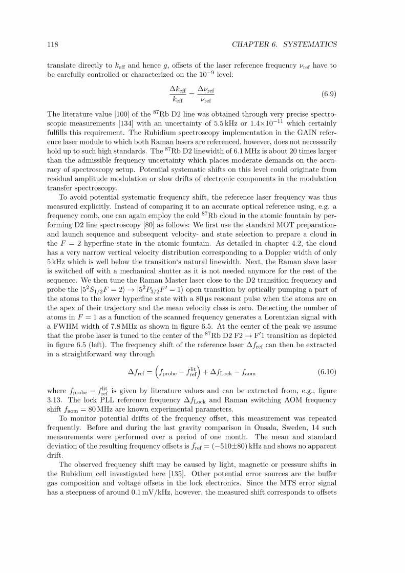
118 CHAPTER 6. SYSTEMATICS
translate directly to keff and hence g, offsets of the laser reference frequency νref have tobe carefully controlled or characterized on the 10−9 level:
∆keffkeff
=∆νrefνref
(6.9)
The literature value [100] of the 87Rb D2 line was obtained through very precise spectro-scopic measurements [134] with an uncertainty of 5.5 kHz or 1.4×10⁻¹¹ which certainlyfulfills this requirement. The Rubidium spectroscopy implementation in the GAIN refer-ence laser module to which both Raman lasers are referenced, however, does not necessarilyhold up to such high standards. The 87Rb D2 linewidth of 6.1 MHz is about 20 times largerthan the admissible frequency uncertainty which places moderate demands on the accu-racy of spectroscopy setup. Potential systematic shifts on this level could originate fromresidual amplitude modulation or slow drifts of electronic components in the modulationtransfer spectroscopy.
To avoid potential systematic frequency shift, the reference laser frequency was thusmeasured explicitly. Instead of comparing it to an accurate optical reference using, e.g. afrequency comb, one can again employ the cold 87Rb cloud in the atomic fountain by per-forming D2 line spectroscopy [80] as follows: We first use the standard MOT preparation-and launch sequence and subsequent velocity- and state selection to prepare a cloud inthe F = 2 hyperfine state in the atomic fountain. As detailed in chapter 4.2, the cloudhas a very narrow vertical velocity distribution corresponding to a Doppler width of only5 kHz which is well below the transition‘s natural linewidth. Next, the Raman slave laseris switched off with a mechanical shutter as it is not needed anymore for the rest of thesequence. We then tune the Raman Master laser close to the D2 transition frequency andprobe the |52S1/2F = 2⟩ → |52P3/2F
′ = 1⟩ open transition by optically pumping a part ofthe atoms to the lower hyperfine state with a 80 µs resonant pulse when the atoms are onthe apex of their trajectory and the mean velocity class is zero. Detecting the number ofatoms in F = 1 as a function of the scanned frequency generates a Lorentzian signal witha FWHM width of 7.8 MHz as shown in figure 6.5. At the center of the peak we assumethat the probe laser is tuned to the center of the 87Rb D2 F2 → F′1 transition as depictedin figure 6.5 (left). The frequency shift of the reference laser ∆fref can then be extractedin a straightforward way through
∆fref =(fprobe − f lit
ref
)+∆fLock − faom (6.10)
where fprobe − f litref is given by literature values and can be extracted from, e.g., figure
3.13. The lock PLL reference frequency ∆fLock and Raman switching AOM frequencyshift faom = 80 MHz are known experimental parameters.
To monitor potential drifts of the frequency offset, this measurement was repeatedfrequently. Before and during the last gravity comparison in Onsala, Sweden, 14 suchmeasurements were performed over a period of one month. The mean and standarddeviation of the resulting frequency offsets is fref = (−510±80) kHz and shows no apparentdrift.
The observed frequency shift may be caused by light, magnetic or pressure shifts inthe Rubidium cell investigated here [135]. Other potential error sources are the buffergas composition and voltage offsets in the lock electronics. Since the MTS error signalhas a steepness of around 0.1 mV/kHz, however, the measured shift corresponds to offsets
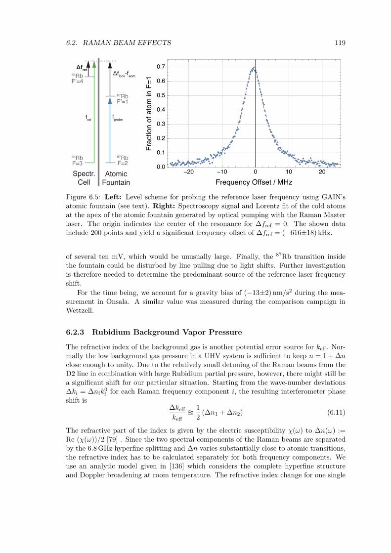
6.2. RAMAN BEAM EFFECTS 119
Spectr.Cell
fprobefref
85Rb
85Rb
87Rb
87Rb
lock-faom
AtomicFountain
- - /=
Figure 6.5: Left: Level scheme for probing the reference laser frequency using GAIN’satomic fountain (see text). Right: Spectroscopy signal and Lorentz fit of the cold atomsat the apex of the atomic fountain generated by optical pumping with the Raman Masterlaser. The origin indicates the center of the resonance for ∆fref = 0. The shown datainclude 200 points and yield a significant frequency offset of ∆fref = (−616±18) kHz.
of several ten mV, which would be unusually large. Finally, the 87Rb transition insidethe fountain could be disturbed by line pulling due to light shifts. Further investigationis therefore needed to determine the predominant source of the reference laser frequencyshift.
For the time being, we account for a gravity bias of (−13±2) nm/s2 during the mea-surement in Onsala. A similar value was measured during the comparison campaign inWettzell.
6.2.3 Rubidium Background Vapor Pressure
The refractive index of the background gas is another potential error source for keff. Nor-mally the low background gas pressure in a UHV system is sufficient to keep n = 1 +∆nclose enough to unity. Due to the relatively small detuning of the Raman beams from theD2 line in combination with large Rubidium partial pressure, however, there might still bea significant shift for our particular situation. Starting from the wave-number deviations∆ki = ∆nik
0i for each Raman frequency component i, the resulting interferometer phase
shift is∆keffkeff
1
2(∆n1 +∆n2) (6.11)
The refractive part of the index is given by the electric susceptibility χ(ω) to ∆n(ω) :=Re (χ(ω))/2 [79] . Since the two spectral components of the Raman beams are separatedby the 6.8 GHz hyperfine splitting and ∆n varies substantially close to atomic transitions,the refractive index has to be calculated separately for both frequency components. Weuse an analytic model given in [136] which considers the complete hyperfine structureand Doppler broadening at room temperature. The refractive index change for one single
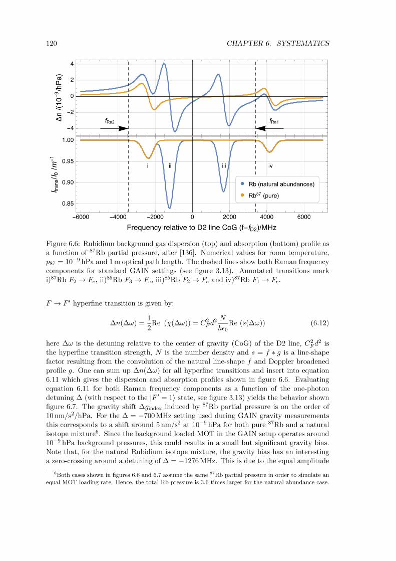
120 CHAPTER 6. SYSTEMATICS
--/(-
/)
fRa1fRa2
- - - ( - )/
//-
i ii iii iv
Rb (natural abundances)Rb87 (pure)
Figure 6.6: Rubidium background gas dispersion (top) and absorption (bottom) profile asa function of 87Rb partial pressure, after [136]. Numerical values for room temperature,p87 = 10−9 hPa and 1 m optical path length. The dashed lines show both Raman frequencycomponents for standard GAIN settings (see figure 3.13). Annotated transitions marki)87Rb F2 → Fe, ii)85Rb F3 → Fe, iii)85Rb F2 → Fe and iv)87Rb F1 → Fe.
F → F ′ hyperfine transition is given by:
∆n(∆ω) =1
2Re (χ(∆ω)) = C2
Fd2 N
ε0Re (s(∆ω)) (6.12)
here ∆ω is the detuning relative to the center of gravity (CoG) of the D2 line, C2Fd
2 isthe hyperfine transition strength, N is the number density and s = f ∗ g is a line-shapefactor resulting from the convolution of the natural line-shape f and Doppler broadenedprofile g. One can sum up ∆n(∆ω) for all hyperfine transitions and insert into equation6.11 which gives the dispersion and absorption profiles shown in figure 6.6. Evaluatingequation 6.11 for both Raman frequency components as a function of the one-photondetuning ∆ (with respect to the |F ′ = 1〉 state, see figure 3.13) yields the behavior shownfigure 6.7. The gravity shift ∆gindex induced by 87Rb partial pressure is on the order of10 nm/s2/hPa. For the ∆ = −700 MHz setting used during GAIN gravity measurementsthis corresponds to a shift around 5 nm/s2 at 10−9 hPa for both pure 87Rb and a naturalisotope mixture6. Since the background loaded MOT in the GAIN setup operates around10−9 hPa background pressures, this could results in a small but significant gravity bias.Note that, for the natural Rubidium isotope mixture, the gravity bias has an interestinga zero-crossing around a detuning of ∆ = −1276 MHz. This is due to the equal amplitude
6Both cases shown in figures 6.6 and 6.7 assume the same 87Rb partial pressure in order to simulate anequal MOT loading rate. Hence, the total Rb pressure is 3.6 times larger for the natural abundance case.
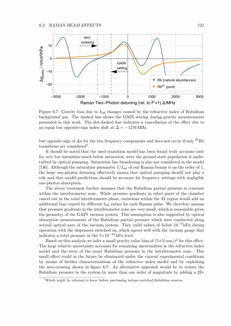
6.2. RAMAN BEAM EFFECTS 121
- - ---
- ( = ) /
///
zerocrossing
GAINsetting
Rb (natural abundances)Rb87 (pure)
Figure 6.7: Gravity bias due to keff changes caused by the refractive index of Rubidiumbackground gas. The dashed line shows the GAIN setting during gravity measurementspresented in this work. The dot-dashed line indicates a cancellation of the effect due toan equal but opposite-sign index shift at ∆ = −1276 MHz.
but opposite sign of ∆n for the two frequency components and does not occur if only 87Rbtransitions are considered7.
It should be noted that the used transition model has been found truly accurate onlyfor very low intensities much below saturation, were the ground state population is undis-turbed by optical pumping. Saturation line broadening is also not considered in the model[136]. Although the saturation parameter I/Isat of our Raman beams is on the order of 1,the large one-photon detuning effectively means that optical pumping should not play arole and that model predictions should be accurate for frequency settings with negligibleone-photon absorption.
The above treatment further assumes that the Rubidium partial pressure is constantwithin the interferometer zone. While pressure gradients in other parts of the chambercancel out in the total interferometer phase, variations within the AI region would add anadditional bias caused by different keff values for each Raman pulse. We therefore assumethat pressure gradients in the interferometer zone are very small, which is reasonable giventhe geometry of the GAIN vacuum system. This assumption is also supported by opticalabsorption measurements of the Rubidium partial pressure which were conducted alongseveral optical axes of the vacuum system. They yield values of below 10−9 hPa duringoperation with the dispensers switched on, which agrees well with the vacuum gauge thatindicates a total pressure at the 5×10⁻¹⁰ hPa level.
Based on this analysis we infer a small gravity value bias of (5±5) nm/s2 for this effect.The large relative uncertainty accounts for remaining uncertainties in the refractive indexmodel and the error of the exact Rubidium pressure in the interferometer zone. Thissmall effect could in the future be eliminated under the current experimental conditionsby means of further characterizations of the refractive index model and by exploitingthe zero-crossing shown in figure 6.7. An alternative approach would be to reduce theRubidium pressure in the system by more than one order of magnitude by adding a 2D-
7Which might be relevant to know before purchasing isotope enriched Rubidium sources.
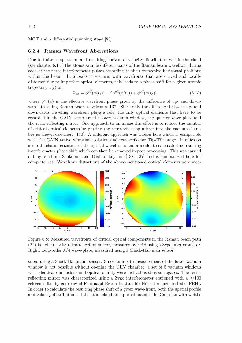
122 CHAPTER 6. SYSTEMATICS
MOT and a differential pumping stage [83].
6.2.4 Raman Wavefront AberrationsDue to finite temperature and resulting horizontal velocity distribution within the cloud(see chapter 6.1.1) the atoms sample different parts of the Raman beam wavefront duringeach of the three interferometer pulses according to their respective horizontal positionswithin the beam. In a realistic scenario with wavefronts that are curved and locallydistorted due to imperfect optical elements, this leads to a phase shift for a given atomictrajectory x(t) of:
Φwf = ϕeff(x(t1))− 2ϕeff(x(t2)) + ϕeff(x(t3)) (6.13)
where ϕeff(x) is the effective wavefront phase given by the difference of up- and down-wards traveling Raman beam wavefronts [137]. Since only the difference between up- anddownwards traveling wavefront plays a role, the only optical elements that have to beregarded in the GAIN setup are the lower vacuum window, the quarter wave plate andthe retro-reflecting mirror. One approach to minimize this effect is to reduce the numberof critical optical elements by putting the retro-reflecting mirror into the vacuum cham-ber as shown elsewhere [130]. A different approach was chosen here which is compatiblewith the GAIN active vibration isolation and retro-reflector Tip/Tilt stage. It relies onaccurate characterization of the optical wavefronts and a model to calculate the resultinginterferometer phase shift which can then be removed in post processing. This was carriedout by Vladimir Schkolnik and Bastian Leykauf [138, 137] and is summarized here forcompleteness. Wavefront distortions of the above-mentioned optical elements were mea-
x / mm
y / mm
−20 −15 −10 −5 0 5 10 15 20−20
−15
−10
−5
0
5
10
15
20
wavefront aberration / λ
−0.04
−0.03
−0.02
−0.01
0
0.01
0.02
0.03
0.04
x / mm
y / mm
−10 −5 0 5 10
−10
−8
−6
−4
−2
0
2
4
6
8
10
wavefront aberration / λ
−0.08
−0.06
−0.04
−0.02
0
0.02
0.04
0.06
Figure 6.8: Measured wavefronts of critical optical components in the Raman beam path(2” diameter). Left: retro-reflection mirror, measured by FBH using a Zygo interferometer.Right: zero-order λ/4 wave-plate, measured using a Shack-Hartman sensor.
sured using a Shack-Hartmann sensor. Since an in-situ measurement of the lower vacuumwindow is not possible without opening the UHV chamber, a set of 5 vacuum windowswith identical dimensions and optical quality were instead used as surrogates. The retro-reflecting mirror was characterized using a Zygo interferometer equipped with a λ/100reference flat by courtesy of Ferdinand-Braun Institut für Höchstfrequenztechnik (FBH).In order to calculate the resulting phase shift of a given wave-front, both the spatial profileand velocity distributions of the atom cloud are approximated to be Gaussian with widths
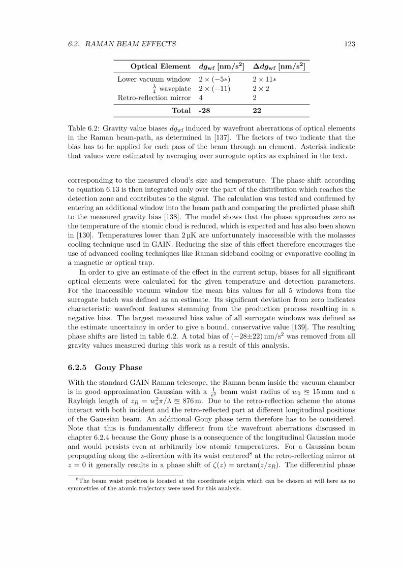
6.2. RAMAN BEAM EFFECTS 123
Optical Element dgwf [nm/s2] ∆dgwf [nm/s2]
Lower vacuum window 2× (−5∗) 2× 11∗λ4 waveplate 2× (−11) 2× 2
Retro-reflection mirror 4 2Total -28 22
Table 6.2: Gravity value biases dgwf induced by wavefront aberrations of optical elementsin the Raman beam-path, as determined in [137]. The factors of two indicate that thebias has to be applied for each pass of the beam through an element. Asterisk indicatethat values were estimated by averaging over surrogate optics as explained in the text.
corresponding to the measured cloud’s size and temperature. The phase shift accordingto equation 6.13 is then integrated only over the part of the distribution which reaches thedetection zone and contributes to the signal. The calculation was tested and confirmed byentering an additional window into the beam path and comparing the predicted phase shiftto the measured gravity bias [138]. The model shows that the phase approaches zero asthe temperature of the atomic cloud is reduced, which is expected and has also been shownin [130]. Temperatures lower than 2 µK are unfortunately inaccessible with the molassescooling technique used in GAIN. Reducing the size of this effect therefore encourages theuse of advanced cooling techniques like Raman sideband cooling or evaporative cooling ina magnetic or optical trap.
In order to give an estimate of the effect in the current setup, biases for all significantoptical elements were calculated for the given temperature and detection parameters.For the inaccessible vacuum window the mean bias values for all 5 windows from thesurrogate batch was defined as an estimate. Its significant deviation from zero indicatescharacteristic wavefront features stemming from the production process resulting in anegative bias. The largest measured bias value of all surrogate windows was defined asthe estimate uncertainty in order to give a bound, conservative value [139]. The resultingphase shifts are listed in table 6.2. A total bias of (−28±22) nm/s2 was removed from allgravity values measured during this work as a result of this analysis.
6.2.5 Gouy Phase
With the standard GAIN Raman telescope, the Raman beam inside the vacuum chamberis in good approximation Gaussian with a 1
e2beam waist radius of w0 ≊ 15 mm and a
Rayleigh length of zR = w2oπ/λ ≊ 876 m. Due to the retro-reflection scheme the atoms
interact with both incident and the retro-reflected part at different longitudinal positionsof the Gaussian beam. An additional Gouy phase term therefore has to be considered.Note that this is fundamentally different from the wavefront aberrations discussed inchapter 6.2.4 because the Gouy phase is a consequence of the longitudinal Gaussian modeand would persists even at arbitrarily low atomic temperatures. For a Gaussian beampropagating along the z-direction with its waist centered8 at the retro-reflecting mirror atz = 0 it generally results in a phase shift of ζ(z) = arctan(z/zR). The differential phase
8The beam waist position is located at the coordinate origin which can be chosen at will here as nosymmetries of the atomic trajectory were used for this analysis.
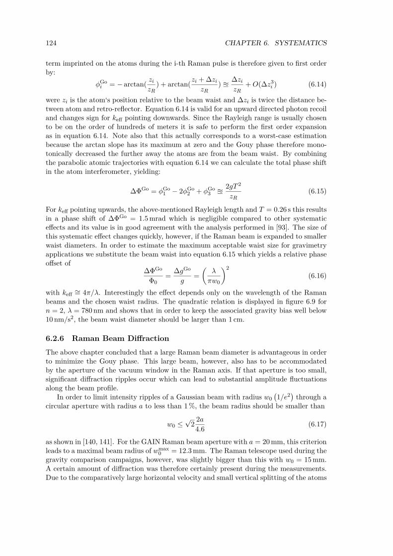
124 CHAPTER 6. SYSTEMATICS
term imprinted on the atoms during the i-th Raman pulse is therefore given to first orderby:
ϕGoi = − arctan( zi
zR) + arctan(zi +∆zi
zR) ≊
∆zizR
+O(∆z3i ) (6.14)
were zi is the atom‘s position relative to the beam waist and ∆zi is twice the distance be-tween atom and retro-reflector. Equation 6.14 is valid for an upward directed photon recoiland changes sign for keff pointing downwards. Since the Rayleigh range is usually chosento be on the order of hundreds of meters it is safe to perform the first order expansionas in equation 6.14. Note also that this actually corresponds to a worst-case estimationbecause the arctan slope has its maximum at zero and the Gouy phase therefore mono-tonically decreased the further away the atoms are from the beam waist. By combiningthe parabolic atomic trajectories with equation 6.14 we can calculate the total phase shiftin the atom interferometer, yielding:
∆ΦGo = ϕGo1 − 2ϕGo
2 + ϕGo3 ≊
2gT 2
zR(6.15)
For keff pointing upwards, the above-mentioned Rayleigh length and T = 0.26 s this resultsin a phase shift of ∆ΦGo = 1.5 mrad which is negligible compared to other systematiceffects and its value is in good agreement with the analysis performed in [93]. The size ofthis systematic effect changes quickly, however, if the Raman beam is expanded to smallerwaist diameters. In order to estimate the maximum acceptable waist size for gravimetryapplications we substitute the beam waist into equation 6.15 which yields a relative phaseoffset of
∆ΦGo
Φ0=
∆gGo
g=
(λ
πw0
)2
(6.16)
with keff ∼= 4π/λ. Interestingly the effect depends only on the wavelength of the Ramanbeams and the chosen waist radius. The quadratic relation is displayed in figure 6.9 forn = 2, λ = 780 nm and shows that in order to keep the associated gravity bias well below10 nm/s2, the beam waist diameter should be larger than 1 cm.
6.2.6 Raman Beam DiffractionThe above chapter concluded that a large Raman beam diameter is advantageous in orderto minimize the Gouy phase. This large beam, however, also has to be accommodatedby the aperture of the vacuum window in the Raman axis. If that aperture is too small,significant diffraction ripples occur which can lead to substantial amplitude fluctuationsalong the beam profile.
In order to limit intensity ripples of a Gaussian beam with radius w0
(1/e2
)through a
circular aperture with radius a to less than 1 %, the beam radius should be smaller than
w0 ≤√22a
4.6(6.17)
as shown in [140, 141]. For the GAIN Raman beam aperture with a = 20 mm, this criterionleads to a maximal beam radius of wmax
0 = 12.3 mm. The Raman telescope used during thegravity comparison campaigns, however, was slightly bigger than this with w0 = 15 mm.A certain amount of diffraction was therefore certainly present during the measurements.Due to the comparatively large horizontal velocity and small vertical splitting of the atoms
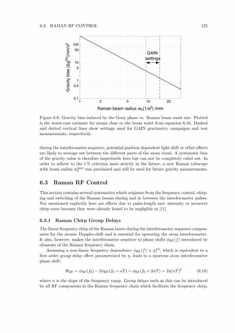
6.3. RAMAN RF CONTROL 125
( / ) /
||//
Figure 6.9: Gravity bias induced by the Gouy phase vs. Raman beam waist size. Plottedis the worst-case estimate for atoms close to the beam waist from equation 6.16. Dashedand dotted vertical lines show settings used for GAIN gravimetry campaigns and testmeasurements, respectively.
during the interferometer sequence, potential position dependent light shift or other effectsare likely to average out between the different parts of the atom cloud. A systematic biasof the gravity value is therefore improbable here but can not be completely ruled out. Inorder to adhere to the 1 % criterion more strictly in the future, a new Raman telescopewith beam radius wmax
0 was purchased and will be used for future gravity measurements.
6.3 Raman RF ControlThis section contains several systematics which originate from the frequency control, chirp-ing and switching of the Raman beams during and in between the interferometer pulses.Not mentioned explicitly here are effects due to pulse-length and -intensity or incorrectchirp rates because they were already found to be negligible in [11].
6.3.1 Raman Chirp Group DelaysThe linear frequency chirp of the Raman lasers during the interferometer sequence compen-sates for the atomic Doppler-shift and is essential for operating the atom interferometer.It also, however, makes the interferometer sensitive to phase shifts φRF(f) introduced byelements of the Raman frequency chain.
Assuming a non-linear frequency dependence φRF(f) ∝ ηf2, which is equivalent to afirst order group delay effect parametrized by η, leads to a spurious atom interferometerphase shift:
ΦRF = φRF(f0)− 2φRF(f0 + αT ) + φRF(f0 + 2αT ) = 2η(αT )2 (6.18)
where α is the slope of the frequency ramp. Group delays such as this can be introducedby all RF components in the Raman frequency chain which facilitate the frequency chirp,
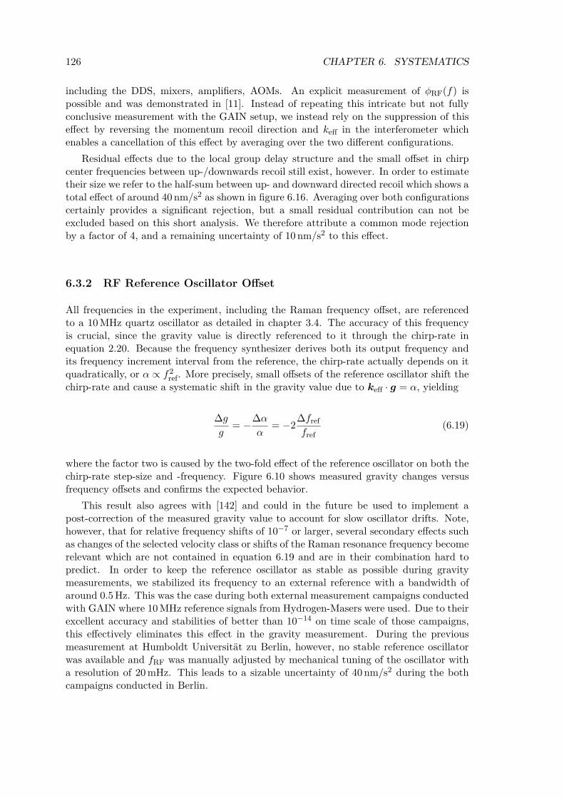
126 CHAPTER 6. SYSTEMATICS
including the DDS, mixers, amplifiers, AOMs. An explicit measurement of ϕRF(f) ispossible and was demonstrated in [11]. Instead of repeating this intricate but not fullyconclusive measurement with the GAIN setup, we instead rely on the suppression of thiseffect by reversing the momentum recoil direction and keff in the interferometer whichenables a cancellation of this effect by averaging over the two different configurations.
Residual effects due to the local group delay structure and the small offset in chirpcenter frequencies between up-/downwards recoil still exist, however. In order to estimatetheir size we refer to the half-sum between up- and downward directed recoil which shows atotal effect of around 40 nm/s2 as shown in figure 6.16. Averaging over both configurationscertainly provides a significant rejection, but a small residual contribution can not beexcluded based on this short analysis. We therefore attribute a common mode rejectionby a factor of 4, and a remaining uncertainty of 10 nm/s2 to this effect.
6.3.2 RF Reference Oscillator Offset
All frequencies in the experiment, including the Raman frequency offset, are referencedto a 10 MHz quartz oscillator as detailed in chapter 3.4. The accuracy of this frequencyis crucial, since the gravity value is directly referenced to it through the chirp-rate inequation 2.20. Because the frequency synthesizer derives both its output frequency andits frequency increment interval from the reference, the chirp-rate actually depends on itquadratically, or α ∝ f2
ref. More precisely, small offsets of the reference oscillator shift thechirp-rate and cause a systematic shift in the gravity value due to keff · g = α, yielding
∆g
g= −∆α
α= −2
∆freffref
(6.19)
where the factor two is caused by the two-fold effect of the reference oscillator on both thechirp-rate step-size and -frequency. Figure 6.10 shows measured gravity changes versusfrequency offsets and confirms the expected behavior.
This result also agrees with [142] and could in the future be used to implement apost-correction of the measured gravity value to account for slow oscillator drifts. Note,however, that for relative frequency shifts of 10−7 or larger, several secondary effects suchas changes of the selected velocity class or shifts of the Raman resonance frequency becomerelevant which are not contained in equation 6.19 and are in their combination hard topredict. In order to keep the reference oscillator as stable as possible during gravitymeasurements, we stabilized its frequency to an external reference with a bandwidth ofaround 0.5 Hz. This was the case during both external measurement campaigns conductedwith GAIN where 10 MHz reference signals from Hydrogen-Masers were used. Due to theirexcellent accuracy and stabilities of better than 10−14 on time scale of those campaigns,this effectively eliminates this effect in the gravity measurement. During the previousmeasurement at Humboldt Universität zu Berlin, however, no stable reference oscillatorwas available and fRF was manually adjusted by mechanical tuning of the oscillator witha resolution of 20 mHz. This leads to a sizable uncertainty of 40 nm/s2 during the bothcampaigns conducted in Berlin.
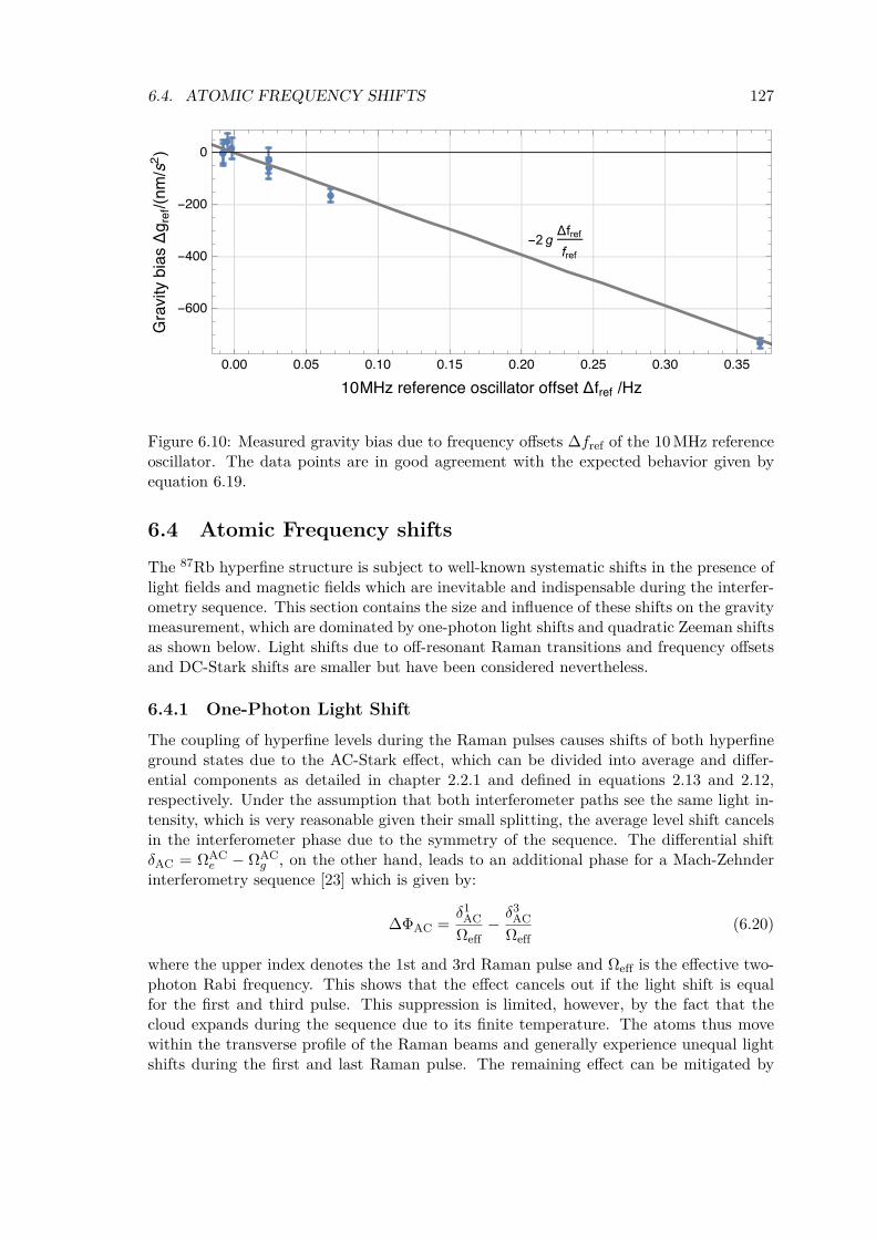
6.4. ATOMIC FREQUENCY SHIFTS 127
---
/
/(/)
-2 g freffref
Figure 6.10: Measured gravity bias due to frequency offsets ∆fref of the 10 MHz referenceoscillator. The data points are in good agreement with the expected behavior given byequation 6.19.
6.4 Atomic Frequency shiftsThe 87Rb hyperfine structure is subject to well-known systematic shifts in the presence oflight fields and magnetic fields which are inevitable and indispensable during the interfer-ometry sequence. This section contains the size and influence of these shifts on the gravitymeasurement, which are dominated by one-photon light shifts and quadratic Zeeman shiftsas shown below. Light shifts due to off-resonant Raman transitions and frequency offsetsand DC-Stark shifts are smaller but have been considered nevertheless.
6.4.1 One-Photon Light ShiftThe coupling of hyperfine levels during the Raman pulses causes shifts of both hyperfineground states due to the AC-Stark effect, which can be divided into average and differ-ential components as detailed in chapter 2.2.1 and defined in equations 2.13 and 2.12,respectively. Under the assumption that both interferometer paths see the same light in-tensity, which is very reasonable given their small splitting, the average level shift cancelsin the interferometer phase due to the symmetry of the sequence. The differential shiftδAC = ΩAC
e − ΩACg , on the other hand, leads to an additional phase for a Mach-Zehnder
interferometry sequence [23] which is given by:
∆ΦAC =δ1ACΩeff
−δ3ACΩeff
(6.20)
where the upper index denotes the 1st and 3rd Raman pulse and Ωeff is the effective two-photon Rabi frequency. This shows that the effect cancels out if the light shift is equalfor the first and third pulse. This suppression is limited, however, by the fact that thecloud expands during the sequence due to its finite temperature. The atoms thus movewithin the transverse profile of the Raman beams and generally experience unequal lightshifts during the first and last Raman pulse. The remaining effect can be mitigated by
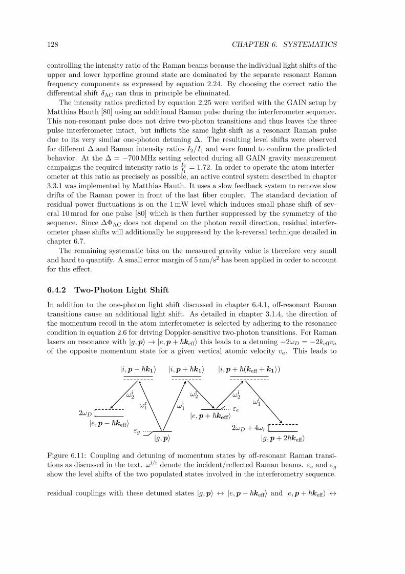
128 CHAPTER 6. SYSTEMATICS
controlling the intensity ratio of the Raman beams because the individual light shifts of theupper and lower hyperfine ground state are dominated by the separate resonant Ramanfrequency components as expressed by equation 2.24. By choosing the correct ratio thedifferential shift δAC can thus in principle be eliminated.
The intensity ratios predicted by equation 2.25 were verified with the GAIN setup byMatthias Hauth [80] using an additional Raman pulse during the interferometer sequence.This non-resonant pulse does not drive two-photon transitions and thus leaves the threepulse interferometer intact, but inflicts the same light-shift as a resonant Raman pulsedue to its very similar one-photon detuning ∆. The resulting level shifts were observedfor different ∆ and Raman intensity ratios I2/I1 and were found to confirm the predictedbehavior. At the ∆ = −700 MHz setting selected during all GAIN gravity measurementcampaigns the required intensity ratio is I2
I1= 1.72. In order to operate the atom interfer-
ometer at this ratio as precisely as possible, an active control system described in chapter3.3.1 was implemented by Matthias Hauth. It uses a slow feedback system to remove slowdrifts of the Raman power in front of the last fiber coupler. The standard deviation ofresidual power fluctuations is on the 1 mW level which induces small phase shift of sev-eral 10 mrad for one pulse [80] which is then further suppressed by the symmetry of thesequence. Since ∆ΦAC does not depend on the photon recoil direction, residual interfer-ometer phase shifts will additionally be suppressed by the k-reversal technique detailed inchapter 6.7.
The remaining systematic bias on the measured gravity value is therefore very smalland hard to quantify. A small error margin of 5 nm/s2 has been applied in order to accountfor this effect.
6.4.2 Two-Photon Light ShiftIn addition to the one-photon light shift discussed in chapter 6.4.1, off-resonant Ramantransitions cause an additional light shift. As detailed in chapter 3.1.4, the direction ofthe momentum recoil in the atom interferometer is selected by adhering to the resonancecondition in equation 2.6 for driving Doppler-sensitive two-photon transitions. For Ramanlasers on resonance with |g,p⟩ → |e,p+ ℏkeff⟩ this leads to a detuning −2ωD = −2keffvaof the opposite momentum state for a given vertical atomic velocity va. This leads to
|g,p⟩εg
|i,p+ ℏk1⟩
ωi1
|i,p− ℏk1⟩
ωr1
|e,p− ℏkeff⟩
ωi2
2ωD |e,p+ ℏkeff⟩εe
ωr2
|i,p+ ℏ(keff + k1⟩)
ωi2
|g,p+ 2ℏkeff⟩
ωr1
2ωD + 4ωr
Figure 6.11: Coupling and detuning of momentum states by off-resonant Raman transi-tions as discussed in the text. ωi/r denote the incident/reflected Raman beams. εe and εgshow the level shifts of the two populated states involved in the interferometry sequence.
residual couplings with these detuned states |g,p⟩ ↔ |e,p− ℏkeff⟩ and |e,p+ ℏkeff⟩ ↔
6.4. ATOMIC FREQUENCY SHIFTS 129
|g,p+ 2ℏkeff⟩ as depicted in figure 6.11 which in turn results in an additional differentiallevel shift [143] of:
δωTPLS =1
ℏ(εe − εg) =
Ω2eff4
(1
±2ωD+
1
±2ωD + 4ωr
)=: ±
Ω2eff
4δD(6.21)
where Ωeff is the effective Rabi frequency of the Raman transition, ωr = ℏk2eff/2m is therecoil frequency and δD abbreviates the effective Doppler shift. Note that δωTPLS changessign when flipping the momentum vector which means that, in contrast to the one-photonlight shift, the k-reversal technique does not reject this effect. The resulting interferometerphase shift can be calculated using the sensitivity function in equation 2.38 and furthersimplified by assuming fix pulse areas of π/2 and π for the Raman pulses which leads toan interferometer phase shift of [143]
ΦTPLS =1
4
(Ω(1)eff
δ(1)D
−Ω(3)eff
δ(3)D
)(6.22)
where Ω(i)eff ,δ
(1)D denote parameters for the i-th Raman pulse. Since the interferometer
sequence in the GAIN atomic fountain is arranged almost symmetrically on the parabolictrajectory of the atoms, the Doppler shift during both the 1st and 3rd pulse is relativelylarge. This strongly suppresses ΦTPLS compared to a configuration where the atoms aresimply dropped and the velocity during the first pulse is thus small. For the standard GAINparameters with T = 0.26 s this leads to a substantial Doppler detuning of 5.8 MHz which,in combination with the effective Rabi frequency of 15 kHz, leads to a very small phaseshift of 1.3 mrad corresponding to 1.3 nm/s2. This is about one order of magnitude smallerthan the targeted accuracy and currently not an issue. For less symmetric configurationsof GAIN, however, where the atomic velocity during the 1st pulse is small this effect canbe much larger and has to be accounted for. Further phase shifts due to couplings fromDoppler-insensitive Raman transitions due to polarization errors might also arise [143]and should be characterized in the future by looking at the Raman spectrum. In orderto account for these potential effects, we assume a total uncertainty of 5 nm/s2 caused bytwo-photon light shifts.
6.4.3 Light shifts due to Raman Frequency Offsets
Interferometer phase shifts can occur if the Raman resonance condition in equation 2.6 isnot met precisely during the atom interferometer sequence. The resulting asymmetry leadsto a sensitivity to non-inertial effects as first reported in [11] and described theoreticallyin [144]. The reported phase shifts due to offsets from the correct Raman frequency forsimilar experimental parameters have a magnitude of roughly 14 nm/s2/kHz.
The importance of this effect for GAIN parameters will briefly be discussed here. Afterthe GAIN velocity selection, which is performed with a Gaussian pulse envelope, the atomicvelocity distribution of the remaining atoms is to a very good approximation representedby a narrow Gaussian which corresponds to a Doppler width of 10 kHz as detailed inchapter 4.2. Scans of the Raman resonance condition yields the required settings withan uncertainty of approximately 500 Hz which results in a gravity value uncertainty of7 nm/s2.
130 CHAPTER 6. SYSTEMATICS
6.4.4 Quadratic Zeeman ShiftLevel shifts caused by magnetic fields are an important error source and have been carefullyconsidered already during the design of the GAIN setup [93, 11]. They are, as a firststep, reduced by only allowing atoms in the magnetically insensitive mF = 0 sub-stateto participate in the atom interferometer by virtue of the selection sequence described inchapter 4.2. The dominant level shift is then caused by the second order Zeeman shiftmodeled by the Breit-Rabi formula [100]. This results in an equal and opposite shift ofthe upper and lower hyperfine ground state leading to a ”clock transition” frequency shiftof
K :=∆ωclkB2
=(gj − gi)
2 µ2B
2ℏ∆Eclk= 2π · 57.5 kHz
mT2 (6.23)
where ∆Eclk is the energy splitting between both states, µB is the Bohr magneton and gjand gi are the fine-structure Landé and nuclear g-factors.
Since the atoms in both arms of the Raman interferometer are in opposite internalstates this causes a differential level shift which can be calculated by evaluating the pathintegral along the unperturbed trajectories in both interferometer arms. In order to find asimple expression that includes the effect of magnetic field gradients across the small split-ting between both interferometer paths we expand the squared magnetic field to secondorder around the classical, mean parabolic trajectory z(t), yielding:
B2(z +∆z) ≊ B2(z) + 2γ(z)B(z)∆z +(γ2(z) + κ(z)B2(z)
)∆z2 + ... (6.24)
where γ := ∂zB and κ := ∂2zB are the vertical gradient and curvature of the magnetic
field, respectively, and ∆z(t) = ±vrec (T − |t− tRa2|) /2 parametrizes the distance of bothinterferometer paths from the mean parabolic trajectory z(t). By evaluating the phaseshift along both paths and using the sensitivity function gs(t) introduced in chapter 2.4the resulting phase shift can be written as an integral along the classical, mean trajectory:
∆ΦB2 = K
∫gs(t)
(B2(t) +
(γ2(t) +B(t)κ(t)
)∆z2(t)
)dt (6.25)
=: ∆ΦmeanB2 +∆Φsplit
B2 (6.26)
with, e.g., B(t) := B(z(t)). The first term shows the dominating effect of magnetic fieldfluctuations along the mean trajectory and the second term a higher order effect due tothe small interferometer path splitting. Note that the first order term in γ is equal in bothinterferometer arms due to the antisymmetry of the (differential) level shift, and thereforecancels out in the measured phase difference.
We will first estimate a worst-case value for the leading order ∆ΦmeanB2 . External
background magnetic fields are strongly reduces in the interferometer region due to the3-layer Mu-Metal shield described in chapter 3.1. A constant bias field of approximatelyB0 ≊ 5µT is applied to provide a well-defined quantization axis and avoid spin-flipsduring the interferometer sequence. Measurements performed in [93] show that spatialfield fluctuations due to external background fields have a magnitude of approximately∆B ≊ 100 nT which was confirmed by Zeeman spectroscopy in the fountain as shown infigure 6.12. In order to give a worst-case estimate of the differential level shift, we assumethat the first half of the atom interferometer is subjected to a constant field B0+∆B andthe second half subjected only to B0.
∆ΦmeanB2 < TK
((B0 +∆B)2 −B2
0
)≊ 2TKB0∆B (6.27)
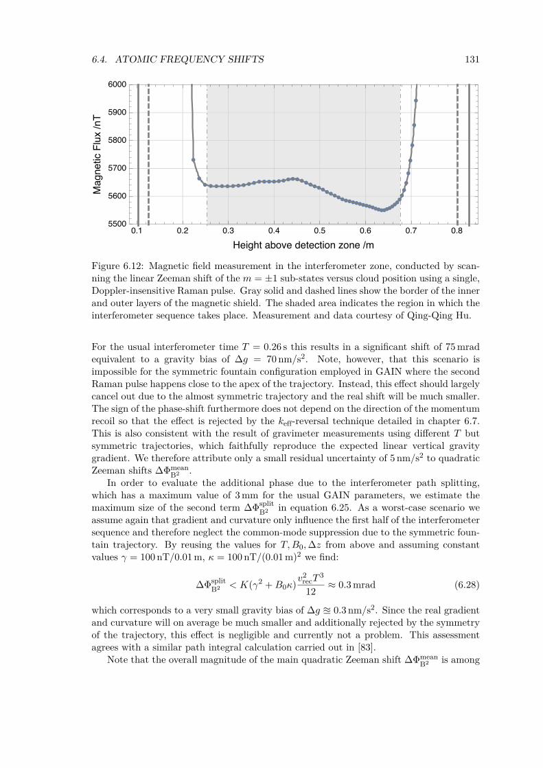
6.4. ATOMIC FREQUENCY SHIFTS 131
/
/
Figure 6.12: Magnetic field measurement in the interferometer zone, conducted by scan-ning the linear Zeeman shift of the m = ±1 sub-states versus cloud position using a single,Doppler-insensitive Raman pulse. Gray solid and dashed lines show the border of the innerand outer layers of the magnetic shield. The shaded area indicates the region in which theinterferometer sequence takes place. Measurement and data courtesy of Qing-Qing Hu.
For the usual interferometer time T = 0.26 s this results in a significant shift of 75 mradequivalent to a gravity bias of ∆g = 70 nm/s2. Note, however, that this scenario isimpossible for the symmetric fountain configuration employed in GAIN where the secondRaman pulse happens close to the apex of the trajectory. Instead, this effect should largelycancel out due to the almost symmetric trajectory and the real shift will be much smaller.The sign of the phase-shift furthermore does not depend on the direction of the momentumrecoil so that the effect is rejected by the keff-reversal technique detailed in chapter 6.7.This is also consistent with the result of gravimeter measurements using different T butsymmetric trajectories, which faithfully reproduce the expected linear vertical gravitygradient. We therefore attribute only a small residual uncertainty of 5 nm/s2 to quadraticZeeman shifts ∆Φmean
B2 .In order to evaluate the additional phase due to the interferometer path splitting,
which has a maximum value of 3 mm for the usual GAIN parameters, we estimate themaximum size of the second term ∆Φsplit
B2 in equation 6.25. As a worst-case scenario weassume again that gradient and curvature only influence the first half of the interferometersequence and therefore neglect the common-mode suppression due to the symmetric foun-tain trajectory. By reusing the values for T,B0,∆z from above and assuming constantvalues γ = 100 nT/0.01 m, κ = 100 nT/(0.01 m)2 we find:
∆ΦsplitB2 < K(γ2 +B0κ)
v2recT3
12≈ 0.3 mrad (6.28)
which corresponds to a very small gravity bias of ∆g 0.3 nm/s2. Since the real gradientand curvature will on average be much smaller and additionally rejected by the symmetryof the trajectory, this effect is negligible and currently not a problem. This assessmentagrees with a similar path integral calculation carried out in [83].
Note that the overall magnitude of the main quadratic Zeeman shift ∆ΦmeanB2 is among
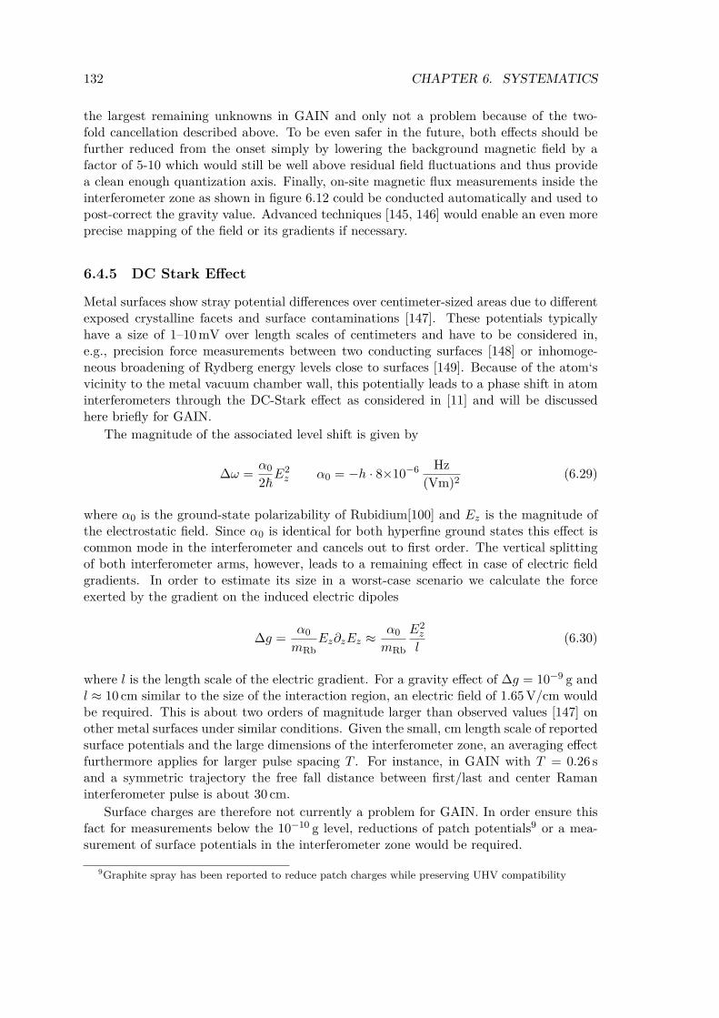
132 CHAPTER 6. SYSTEMATICS
the largest remaining unknowns in GAIN and only not a problem because of the two-fold cancellation described above. To be even safer in the future, both effects should befurther reduced from the onset simply by lowering the background magnetic field by afactor of 5-10 which would still be well above residual field fluctuations and thus providea clean enough quantization axis. Finally, on-site magnetic flux measurements inside theinterferometer zone as shown in figure 6.12 could be conducted automatically and used topost-correct the gravity value. Advanced techniques [145, 146] would enable an even moreprecise mapping of the field or its gradients if necessary.
6.4.5 DC Stark Effect
Metal surfaces show stray potential differences over centimeter-sized areas due to differentexposed crystalline facets and surface contaminations [147]. These potentials typicallyhave a size of 1–10 mV over length scales of centimeters and have to be considered in,e.g., precision force measurements between two conducting surfaces [148] or inhomoge-neous broadening of Rydberg energy levels close to surfaces [149]. Because of the atom‘svicinity to the metal vacuum chamber wall, this potentially leads to a phase shift in atominterferometers through the DC-Stark effect as considered in [11] and will be discussedhere briefly for GAIN.
The magnitude of the associated level shift is given by
∆ω =α0
2ℏE2
z α0 = −h · 8×10⁻⁶ Hz(Vm)2 (6.29)
where α0 is the ground-state polarizability of Rubidium[100] and Ez is the magnitude ofthe electrostatic field. Since α0 is identical for both hyperfine ground states this effect iscommon mode in the interferometer and cancels out to first order. The vertical splittingof both interferometer arms, however, leads to a remaining effect in case of electric fieldgradients. In order to estimate its size in a worst-case scenario we calculate the forceexerted by the gradient on the induced electric dipoles
∆g =α0
mRbEz∂zEz ≈
α0
mRb
E2z
l(6.30)
where l is the length scale of the electric gradient. For a gravity effect of ∆g = 10−9 g andl ≈ 10 cm similar to the size of the interaction region, an electric field of 1.65 V/cm wouldbe required. This is about two orders of magnitude larger than observed values [147] onother metal surfaces under similar conditions. Given the small, cm length scale of reportedsurface potentials and the large dimensions of the interferometer zone, an averaging effectfurthermore applies for larger pulse spacing T . For instance, in GAIN with T = 0.26 sand a symmetric trajectory the free fall distance between first/last and center Ramaninterferometer pulse is about 30 cm.
Surface charges are therefore not currently a problem for GAIN. In order ensure thisfact for measurements below the 10−10 g level, reductions of patch potentials9 or a mea-surement of surface potentials in the interferometer zone would be required.
9Graphite spray has been reported to reduce patch charges while preserving UHV compatibility
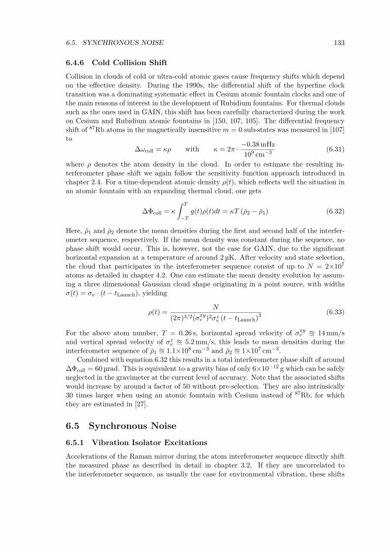
6.5. SYNCHRONOUS NOISE 133
6.4.6 Cold Collision ShiftCollision in clouds of cold or ultra-cold atomic gases cause frequency shifts which dependon the effective density. During the 1990s, the differential shift of the hyperfine clocktransition was a dominating systematic effect in Cesium atomic fountain clocks and one ofthe main reasons of interest in the development of Rubidium fountains. For thermal cloudssuch as the ones used in GAIN, this shift has been carefully characterized during the workon Cesium and Rubidium atomic fountains in [150, 107, 105]. The differential frequencyshift of 87Rb atoms in the magnetically insensitive m = 0 sub-states was measured in [107]to
∆ωcoll = κρ with κ = 2π · −0.38 mHz109 cm−3 (6.31)
where ρ denotes the atom density in the cloud. In order to estimate the resulting in-terferometer phase shift we again follow the sensitivity function approach introduced inchapter 2.4. For a time-dependent atomic density ρ(t), which reflects well the situation inan atomic fountain with an expanding thermal cloud, one gets
∆Φcoll = κ
∫ T
−Tg(t)ρ(t)dt = κT (ρ2 − ρ1) (6.32)
Here, ρ1 and ρ2 denote the mean densities during the first and second half of the interfer-ometer sequence, respectively. If the mean density was constant during the sequence, nophase shift would occur. This is, however, not the case for GAIN, due to the significanthorizontal expansion at a temperature of around 2 µK. After velocity and state selection,the cloud that participates in the interferometer sequence consist of up to N = 2×10⁷
atoms as detailed in chapter 4.2. One can estimate the mean density evolution by assum-ing a three dimensional Gaussian cloud shape originating in a point source, with widthsσ(t) = σv · (t− tLaunch), yielding
ρ(t) =N
(2π)3/2(σxyv )2σz
v (t− tLaunch)3 (6.33)
For the above atom number, T = 0.26 s, horizontal spread velocity of σxyv ≊ 14 mm/s
and vertical spread velocity of σzv ≊ 5.2 mm/s, this leads to mean densities during the
interferometer sequence of ρ1 ≊ 1.1×108 cm−3 and ρ2 ≊ 1×107 cm−3.Combined with equation 6.32 this results in a total interferometer phase shift of around
∆Φcoll = 60 µrad. This is equivalent to a gravity bias of only 6×10⁻¹² g which can be safelyneglected in the gravimeter at the current level of accuracy. Note that the associated shiftswould increase by around a factor of 50 without pre-selection. They are also intrinsically30 times larger when using an atomic fountain with Cesium instead of 87Rb, for whichthey are estimated in [27].
6.5 Synchronous Noise6.5.1 Vibration Isolator ExcitationsAccelerations of the Raman mirror during the atom interferometer sequence directly shiftthe measured phase as described in detail in chapter 3.2. If they are uncorrelated tothe interferometer sequence, as usually the case for environmental vibration, these shifts
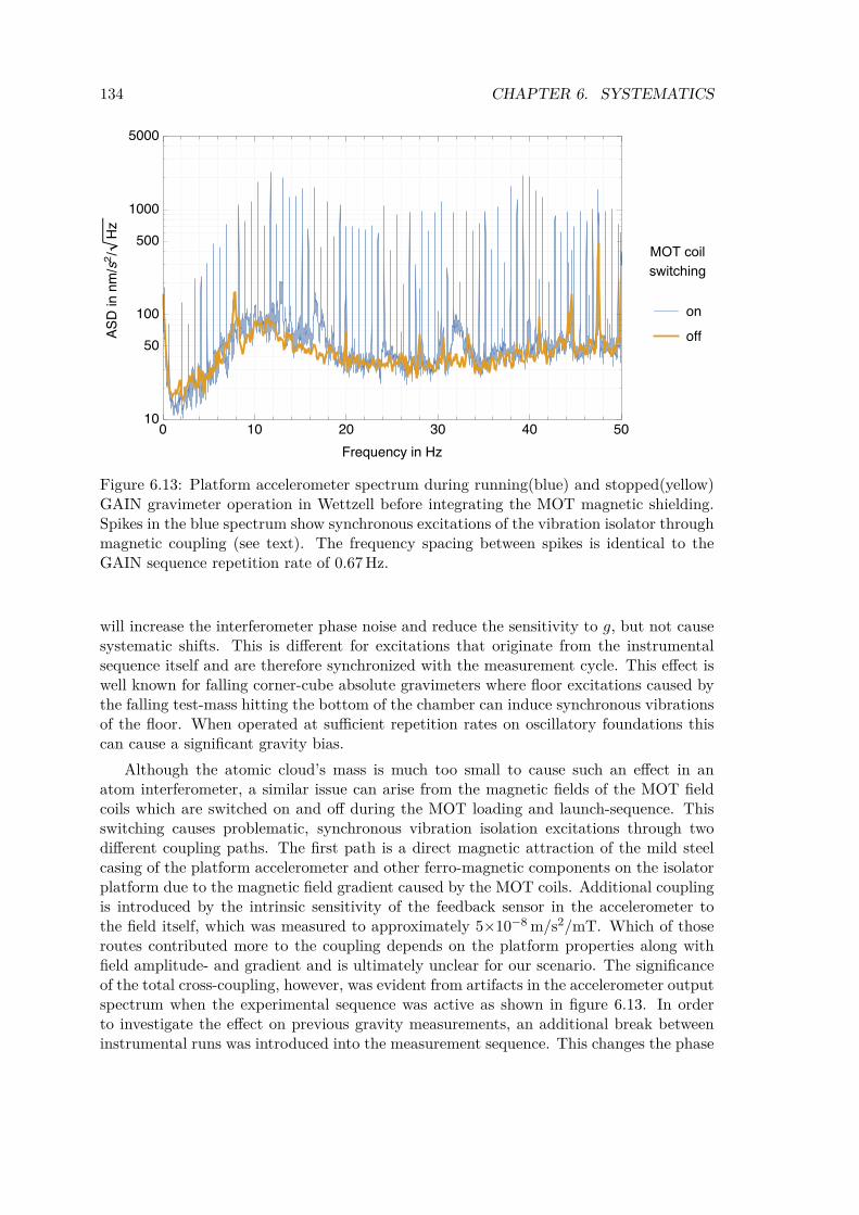
134 CHAPTER 6. SYSTEMATICS// MOT coil
switching
Figure 6.13: Platform accelerometer spectrum during running(blue) and stopped(yellow)GAIN gravimeter operation in Wettzell before integrating the MOT magnetic shielding.Spikes in the blue spectrum show synchronous excitations of the vibration isolator throughmagnetic coupling (see text). The frequency spacing between spikes is identical to theGAIN sequence repetition rate of 0.67 Hz.
will increase the interferometer phase noise and reduce the sensitivity to g, but not causesystematic shifts. This is different for excitations that originate from the instrumentalsequence itself and are therefore synchronized with the measurement cycle. This effect iswell known for falling corner-cube absolute gravimeters where floor excitations caused bythe falling test-mass hitting the bottom of the chamber can induce synchronous vibrationsof the floor. When operated at sufficient repetition rates on oscillatory foundations thiscan cause a significant gravity bias.
Although the atomic cloud’s mass is much too small to cause such an effect in anatom interferometer, a similar issue can arise from the magnetic fields of the MOT fieldcoils which are switched on and off during the MOT loading and launch-sequence. Thisswitching causes problematic, synchronous vibration isolation excitations through twodifferent coupling paths. The first path is a direct magnetic attraction of the mild steelcasing of the platform accelerometer and other ferro-magnetic components on the isolatorplatform due to the magnetic field gradient caused by the MOT coils. Additional couplingis introduced by the intrinsic sensitivity of the feedback sensor in the accelerometer tothe field itself, which was measured to approximately 5×10⁻⁸ m/s2/mT. Which of thoseroutes contributed more to the coupling depends on the platform properties along withfield amplitude- and gradient and is ultimately unclear for our scenario. The significanceof the total cross-coupling, however, was evident from artifacts in the accelerometer outputspectrum when the experimental sequence was active as shown in figure 6.13. In orderto investigate the effect on previous gravity measurements, an additional break betweeninstrumental runs was introduced into the measurement sequence. This changes the phase
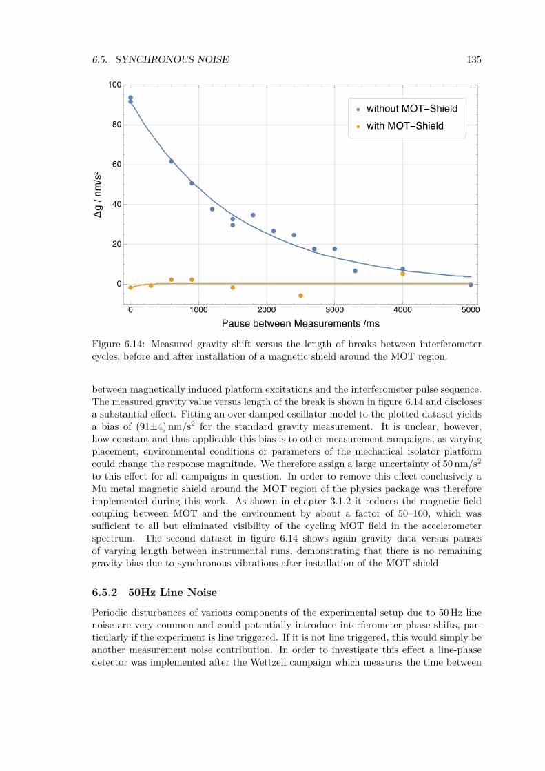
6.5. SYNCHRONOUS NOISE 135
--
/
//
Figure 6.14: Measured gravity shift versus the length of breaks between interferometercycles, before and after installation of a magnetic shield around the MOT region.
between magnetically induced platform excitations and the interferometer pulse sequence.The measured gravity value versus length of the break is shown in figure 6.14 and disclosesa substantial effect. Fitting an over-damped oscillator model to the plotted dataset yieldsa bias of (91±4) nm/s2 for the standard gravity measurement. It is unclear, however,how constant and thus applicable this bias is to other measurement campaigns, as varyingplacement, environmental conditions or parameters of the mechanical isolator platformcould change the response magnitude. We therefore assign a large uncertainty of 50 nm/s2
to this effect for all campaigns in question. In order to remove this effect conclusively aMu metal magnetic shield around the MOT region of the physics package was thereforeimplemented during this work. As shown in chapter 3.1.2 it reduces the magnetic fieldcoupling between MOT and the environment by about a factor of 50–100, which wassufficient to all but eliminated visibility of the cycling MOT field in the accelerometerspectrum. The second dataset in figure 6.14 shows again gravity data versus pausesof varying length between instrumental runs, demonstrating that there is no remaininggravity bias due to synchronous vibrations after installation of the MOT shield.
6.5.2 50Hz Line Noise
Periodic disturbances of various components of the experimental setup due to 50 Hz linenoise are very common and could potentially introduce interferometer phase shifts, par-ticularly if the experiment is line triggered. If it is not line triggered, this would simply beanother measurement noise contribution. In order to investigate this effect a line-phasedetector was implemented after the Wettzell campaign which measures the time between
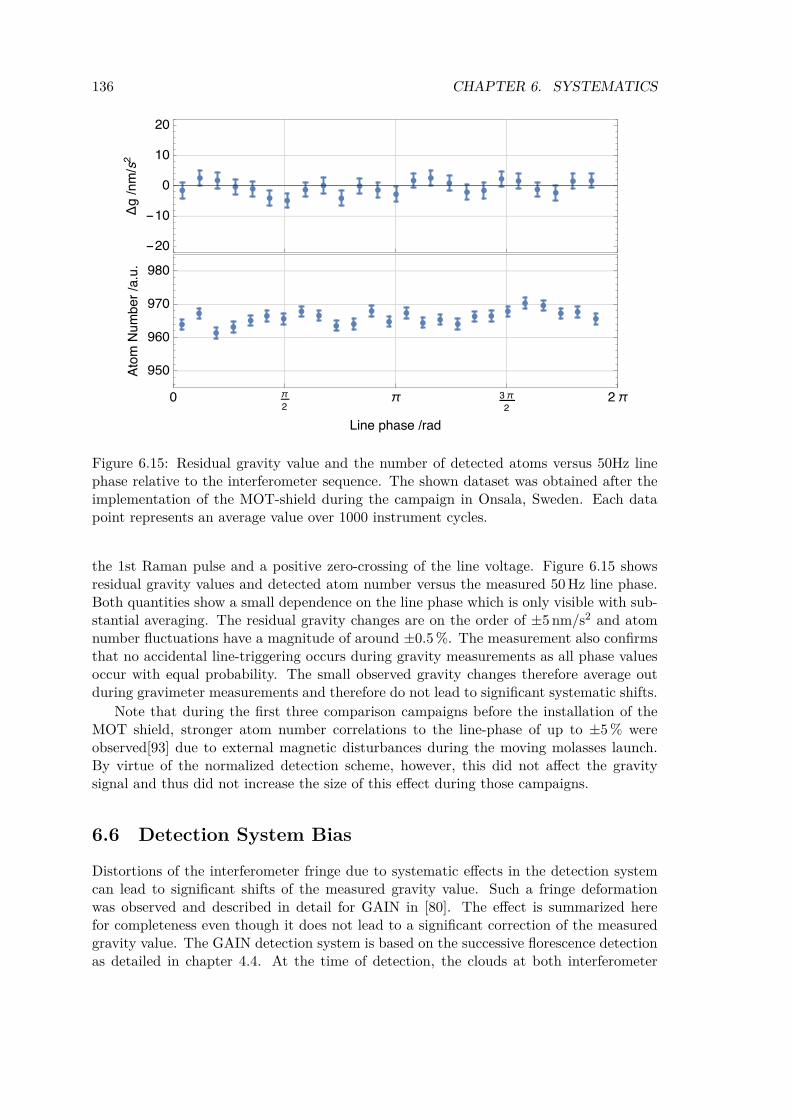
136 CHAPTER 6. SYSTEMATICS
--//
/
/
Figure 6.15: Residual gravity value and the number of detected atoms versus 50Hz linephase relative to the interferometer sequence. The shown dataset was obtained after theimplementation of the MOT-shield during the campaign in Onsala, Sweden. Each datapoint represents an average value over 1000 instrument cycles.
the 1st Raman pulse and a positive zero-crossing of the line voltage. Figure 6.15 showsresidual gravity values and detected atom number versus the measured 50 Hz line phase.Both quantities show a small dependence on the line phase which is only visible with sub-stantial averaging. The residual gravity changes are on the order of ±5 nm/s2 and atomnumber fluctuations have a magnitude of around ±0.5 %. The measurement also confirmsthat no accidental line-triggering occurs during gravity measurements as all phase valuesoccur with equal probability. The small observed gravity changes therefore average outduring gravimeter measurements and therefore do not lead to significant systematic shifts.
Note that during the first three comparison campaigns before the installation of theMOT shield, stronger atom number correlations to the line-phase of up to ±5 % wereobserved[93] due to external magnetic disturbances during the moving molasses launch.By virtue of the normalized detection scheme, however, this did not affect the gravitysignal and thus did not increase the size of this effect during those campaigns.
6.6 Detection System Bias
Distortions of the interferometer fringe due to systematic effects in the detection systemcan lead to significant shifts of the measured gravity value. Such a fringe deformationwas observed and described in detail for GAIN in [80]. The effect is summarized herefor completeness even though it does not lead to a significant correction of the measuredgravity value. The GAIN detection system is based on the successive florescence detectionas detailed in chapter 4.4. At the time of detection, the clouds at both interferometer
6.7. MOMENTUM RECOIL REVERSAL TECHNIQUE 137
output ports have a position offset of 0.4 mm due to the ℏkeff momentum difference afterthe last interferometer pulse. This is smaller than the vertical size of each cloud andleads to a large overlap which means that the second pulse yields roughly the total atomnumber10. The detection pulses for both output ports are separated by 400 µs whichcorresponds to a free fall distance of 1.4 mm. Due to the Gaussian-shaped excitationbeam and inhomogeneous imaging onto the PMT aperture this results in unequal detectionefficiencies for both clouds which slightly distorts the interferometer fringe output. Thisdistortion is maximal on the flanks of the fringe pattern and leaves the maximum/minimumuntouched. When operating at mid-fringe for optimal phase sensitivity, [80] predictedresulting gravity shifts as large as ±70 nm/s2. Fortunately this shift is rejected whenaveraging over the left and right flank with respect to the fringe maximum, and in thiscase enters merely as a noise term which can be easily identified in the spectral density ofthe gravity time series. All gravity measurements during this work were performed usingsymmetric operation on both sides of the interferometer fringe and should therefore notbe affected.
Residual effects might occur, however, during relatively fast tidal gravity changes whichtemporarily offset the operating point from mid-fringe due to interferometer phase controllag. This could mimic effective time delays as observed in [80] and discussed in detail inchapter 5.5.2. In order to eliminate this issue before the last measurement campaign anadditional feed-forward path was implemented. It uses a tidal gravity model11 to keep theinterferometer operating exactly at mid-fringe even during relatively rapid tidal gravitychanges. The feedback path therefore only has to compensate slow gravity variations dueto environmental effects not contained in the model.
Due to the symmetric mid-fringe operation, detection system biases should thereforenot be a problem.
6.7 Momentum Recoil Reversal Technique
As mentioned throughout the discussion some of the above systematics change their signwith the overall interferometer phase when the direction of the momentum recoil is re-versed, and others do not. In order to formalize this we categorized all systematic contri-butions into Φ− and Φ+. The overall atom interferometer phase including those effects isthen given by [80]
Φ↑/↓total = ±
(keff · gT 2 ± Φrec +Φ−
)+Φ+ (6.34)
Here, Φrec = γvrecT/2 denotes an additional phase shift due to the slightly different atomictrajectories for both configurations which for GAIN parameters translates to a differenceof nearly 5 mrad. Additional path integral terms of the interferometer phase shift wereneglected here due to their small size. Most of the systematic effects discussed in theabove chapters depend on the recoil direction and contribute to Φ−. Φ+ consists mostnotably of RF group delay, one-photon light shift and quadratic Zeeman shifts which canthus be separated from the gravity induced phase shift by regarding the half-difference
10Specifically, the second detection pulse takes place symmetrically between both clouds, around whichthe first and last pulse are spaced by the cloud distance.
11This does not restrict the choice of potential measurement sites as simple synthetic models sufficewhich can be generated automatically for most locations without prior gravity registrations.
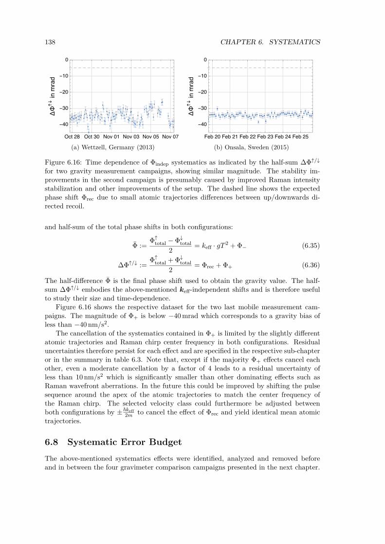
138 CHAPTER 6. SYSTEMATICS
----
(a) Wettzell, Germany (2013)
----
(b) Onsala, Sweden (2015)
Figure 6.16: Time dependence of Φindep systematics as indicated by the half-sum ∆Φ↑/↓
for two gravity measurement campaigns, showing similar magnitude. The stability im-provements in the second campaign is presumably caused by improved Raman intensitystabilization and other improvements of the setup. The dashed line shows the expectedphase shift Φrec due to small atomic trajectories differences between up/downwards di-rected recoil.
and half-sum of the total phase shifts in both configurations:
Φ :=Φ↑
total − Φ↓total
2= keff · gT 2 +Φ− (6.35)
∆Φ↑/↓ :=Φ↑
total +Φ↓total
2= Φrec +Φ+ (6.36)
The half-difference Φ is the final phase shift used to obtain the gravity value. The half-sum ∆Φ↑/↓ embodies the above-mentioned keff-independent shifts and is therefore usefulto study their size and time-dependence.
Figure 6.16 shows the respective dataset for the two last mobile measurement cam-paigns. The magnitude of Φ+ is below −40 mrad which corresponds to a gravity bias ofless than −40 nm/s2.
The cancellation of the systematics contained in Φ+ is limited by the slightly differentatomic trajectories and Raman chirp center frequency in both configurations. Residualuncertainties therefore persist for each effect and are specified in the respective sub-chapteror in the summary in table 6.3. Note that, except if the majority Φ+ effects cancel eachother, even a moderate cancellation by a factor of 4 leads to a residual uncertainty ofless than 10 nm/s2 which is significantly smaller than other dominating effects such asRaman wavefront aberrations. In the future this could be improved by shifting the pulsesequence around the apex of the atomic trajectories to match the center frequency ofthe Raman chirp. The selected velocity class could furthermore be adjusted betweenboth configurations by ±keff
2m to cancel the effect of Φrec and yield identical mean atomictrajectories.
6.8 Systematic Error BudgetThe above-mentioned systematics effects were identified, analyzed and removed beforeand in between the four gravimeter comparison campaigns presented in the next chapter.
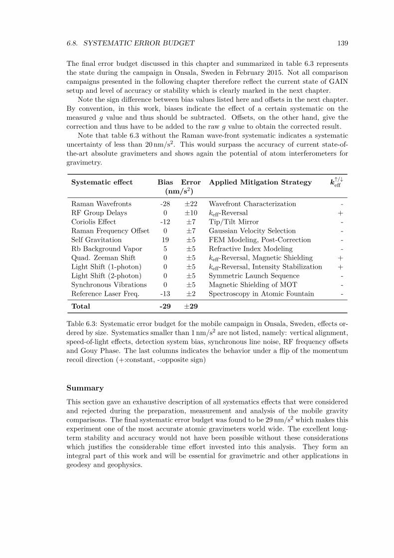
6.8. SYSTEMATIC ERROR BUDGET 139
The final error budget discussed in this chapter and summarized in table 6.3 representsthe state during the campaign in Onsala, Sweden in February 2015. Not all comparisoncampaigns presented in the following chapter therefore reflect the current state of GAINsetup and level of accuracy or stability which is clearly marked in the next chapter.
Note the sign difference between bias values listed here and offsets in the next chapter.By convention, in this work, biases indicate the effect of a certain systematic on themeasured g value and thus should be subtracted. Offsets, on the other hand, give thecorrection and thus have to be added to the raw g value to obtain the corrected result.
Note that table 6.3 without the Raman wave-front systematic indicates a systematicuncertainty of less than 20 nm/s2. This would surpass the accuracy of current state-of-the-art absolute gravimeters and shows again the potential of atom interferometers forgravimetry.
Systematic effect Bias Error Applied Mitigation Strategy k↑/↓eff
(nm/s2)Raman Wavefronts -28 ±22 Wavefront Characterization -RF Group Delays 0 ±10 keff-Reversal +Coriolis Effect -12 ±7 Tip/Tilt Mirror -Raman Frequency Offset 0 ±7 Gaussian Velocity Selection -Self Gravitation 19 ±5 FEM Modeling, Post-Correction -Rb Background Vapor 5 ±5 Refractive Index Modeling -Quad. Zeeman Shift 0 ±5 keff-Reversal, Magnetic Shielding +Light Shift (1-photon) 0 ±5 keff-Reversal, Intensity Stabilization +Light Shift (2-photon) 0 ±5 Symmetric Launch Sequence -Synchronous Vibrations 0 ±5 Magnetic Shielding of MOT -Reference Laser Freq. -13 ±2 Spectroscopy in Atomic Fountain -Total -29 ±29
Table 6.3: Systematic error budget for the mobile campaign in Onsala, Sweden, effects or-dered by size. Systematics smaller than 1 nm/s2 are not listed, namely: vertical alignment,speed-of-light effects, detection system bias, synchronous line noise, RF frequency offsetsand Gouy Phase. The last columns indicates the behavior under a flip of the momentumrecoil direction (+:constant, -:opposite sign)
SummaryThis section gave an exhaustive description of all systematics effects that were consideredand rejected during the preparation, measurement and analysis of the mobile gravitycomparisons. The final systematic error budget was found to be 29 nm/s2 which makes thisexperiment one of the most accurate atomic gravimeters world wide. The excellent long-term stability and accuracy would not have been possible without these considerationswhich justifies the considerable time effort invested into this analysis. They form anintegral part of this work and will be essential for gravimetric and other applications ingeodesy and geophysics.

140 CHAPTER 6. SYSTEMATICS
Chapter 7
Conclusion and Outlook
The main objective of this thesis was to improve the performance characteristics of theGAIN setup for mobile applications in geodesy and gravimetry, and to increase the ab-solute accuracy of the measured gravity value to the 10−9 g level. To this end, severalinstrumental improvements were carried out by the author and described in this thesis.
The Raman retro-reflector was equipped with a Piezo Tip/Tilt mirror system whichwas then used to compensate the Coriolis effect and to perform automatic auto-collimationof the reflected beam back into the Raman fiber. This enabled, in combination with theimplementation of a motorized Raman beam steering system, the automatic alignmentof the GAIN measurement axis with gravity. Other major improvements of the setupwere the integration of a cleaner, larger Rubidium source and new programming hardwarefor the Raman DDS frequency synthesizers, which now use fast FPGA processing toenable arbitrary frequency and phase control during the sequence. A magnetic shieldaround the MOT zone of the physics package was also implemented to remove magneticexcitation of the vibration isolation system which had previously caused major systematicand random perturbations. Finally, a post-correction algorithm for residual vibrationswas implemented and applied subsequently to all conducted measurement campaigns.This significantly increased the sensitivity to g and lead to major new insights into theobserved GAIN measurement noise.
During and after the implementation of these instrumental improvements, four compar-ison campaigns between GAIN and different state-of-the-art relative and absolute gravime-ters were conducted. This included comparisons to relative spring-based and supercon-ducting gravimeters as well as the state-of-the-art falling corner-cube gravimeter FG5X-220. The last two comparisons took place at remote locations in Wettzell, Germany andOnsala, Sweden to verify the mobility of the GAIN setup. The presented analysis of all fourmeasurement campaigns shows the improvement in long-term stability and accuracy overtime as systematic effects were increasingly suppressed or compensated in post-processing.The best performance was reached in the last campaign with an absolute accuracy due tothe systematic error budget of 37 nm/s2, sensitivity of 85 nm/s2/
√Hz and current world-
record long-term stability of 0.4 nm/s2, or 4×10⁻¹¹ g, after one day of integration time.These numbers compare very well with other mobile state-of-the-art atomic gravimeters[65] and make GAIN one of the most advanced devices of this kind to date.
The comparisons between GAIN and the FG5X-220 furthermore unveiled interestingdifferences in the general characteristics of atomic and falling corner-cube gravimeters.Despite the good agreement in the measured gravity values, the repeatedly larger result
141

142 CHAPTER 7. CONCLUSION AND OUTLOOK
from GAIN in combination with slightly elevated values also measured by other atomicgravimeters [65, 13] indicates that hidden systematic offsets in at least one class of instru-ments might still exist today. Further investigations are needed here, but this point alsoillustrates that the comparison of different absolute gravimeter implementations is notonly interesting in its own right, but essential to find and remove these hidden systemat-ics. Since, until recently, falling corner-cube gravimeters such as the Microg-LaCoste FG5completely dominated this field, the advent of atomic gravimeters in geodesy will certainlylead to a strongly increased confidence in the accuracy of future gravity networks.
Another characteristic difference is the resilience against environmental noise. Becauseof the increased micro-seismic noise level during the campaigns in Onsala and Berlin, mea-surement noise of the FG5X was strongly increased due to technical limitations of theFG5(X) super-spring [110] which decouples its inertial reference mirror from the environ-ment. GAIN was, due to its higher repetition rate and more efficacious vibration isolationsystem, not affected by elevated micro-seismic noise and showed much lower measurementnoise than the FG5 under those conditions. In contrast to GAIN or other atomic gravime-ters, falling corner-cube instruments also require a solid concrete foundation to achieve ad-equate performance as the lifting and falling of the corner-cube induces vibrations. GAINdoes not possess this restriction as no moving parts exist in the physics package. Bothadvantages apply to atomic gravimeters in general and provide access to a much largerset of potential measurement sites for state-of-the-art absolute gravimetry. The ability ofatomic gravimeters to perform continuous gravity registrations over long periods of timein combination with reduced measurement noise furthermore enables applications whichwere before restricted to relative gravimeters, such as tidal model characterizations orthe investigation of ground water induced gravity effects. Falling corner-cube instrumentspractically never operate continuously over extended periods of time to prevent wear andtear of the complicated mechanical dropping system. Although GAIN can not yet reachthe excellent short-term sensitivity of superconducting gravimeters it has already providedunique sets of continuous absolute gravity data over weeks with a noise level similar torelative spring-based gravimeters without the long-term drift. Future improvements ofGAIN‘s short- and long-term stability as well as its accuracy and mobility will make iteven more attractive for the above applications in geodesy. These improvements shouldfirst focus on reducing the excess noise contribution described in this work and a furtherreduction of Raman wavefront aberrations as well as other remaining systematics. Ad-vanced concepts to improve the sensitivity such as interleaved interferometry [151] anddead-time free measurements with two atomic species or isotopes [152] have been demon-strated and might provide a further quantum leap in sensitivity. In order to exploit thispotential for geodesy on a larger scale, commercialized atomic gravimeters [75, 76, 77]are starting to appear on the market [153]. The robust and scalable architecture of atominterferometers further enables applications under harsh environments where spring-basedrelative gravimeters reach fundamental limitations, which has spurred the development ofspecialized atomic sensors for airborne, shipborne [152, 154] or borehole gravimeters. Asthe broader potential of inertial sensor and specifically gravimeters based on atom inter-ferometry is completely open, the future will show plenty of interesting new applicationsof this versatile concept.

Appendices
143


Appendix A
MOT Photograph
Figure A.1: Photograph of the MOT system just before installation of the MOT shield.The atomic fountain system is fully connected and in operation with optimized launchtemperature using the compensation coils wound around the MOT chamber as specified infigure 3.3. Fluorescence light from the 87Rb MOT is visible through the central viewport.
145

146 APPENDIX A. MOT PHOTOGRAPH
Appendix B
Measurement Campaigns
This chapter lists all parameters required to reproduced the results of the gravity com-parison campaigns. This includes, for every campaign, the used tidal parameters, sourceand admittance factor used for air-pressure correction, the height of GAIN detection zoneand GAIN effective measurement height, and the vertical gravity gradient at this height.All tidal model and polar motion correction calculation have been performed with Tsoft[47]. The polar motion correction was also computed with the same software using polecoordinates from IERS at http://hpiers.obspm.fr/iers/eop/eopc04_14/.
B.1 Air-Pressure CorrectionDuring each campaign the atmospheric loading effect was calculated from local air pres-sure records using an admittance factor ap which leads to a simple gravity correction of∆gair(t) = ap
(p(t)− pstd
), where pstd is the base pressure at a given altitude according
to the standard barometric formula:
p(h) = 1013.24 hPa exp(1− 0.0065h
288.15 m
)5.255
(B.1)
Since the admittance factor ap changes slightly for different stations it is given for each ofthe four measurement campaigns.
If air pressure data from a nearby weather station at different altitude was used forair pressure correction, an offset ∆p = p(hgravi)− p(hstation) was added to the respectiverecords to account for the different base pressure level at the campaign measurement site.
147

148 APPENDIX B. MEASUREMENT CAMPAIGNS
B.2 Campaign 1: GAIN and gPhone (Berlin, 2012)Locations The measurement was performed at Humboldt Universität zu Berlin in Lise-MeitnerBuilding, Newtonstr. 15, D-12489 Berlin in room 1‘601.
latitude longitude altitude GAIN detection GAIN effective[°N] [°E] [m] height [m] meas. height [m]
52.43337 13.53062 39.65 0.812±0.003 1.398±0.003
Tidal ModelThe earth tide parameters for Berlin were provided by IfE [108]. The listed parametersinclude the effect of ocean loading, e.g. no additional loading correction was performed.
Frequency Frequency Amplitude Phase Tide Symbolmin. [cyc/d] max. [cyc/d] [°]
0.0 0.000001 1.0 0.0 DC0.0001 0.249951 1.1792 -0.0222 Long
0.721500 0.906315 1.14970 -0.1150 Q10.921941 0.974188 1.14870 0.1114 O10.989049 0.998028 1.14800 0.1711 P10.999853 1.216397 1.13360 0.1122 K11.719381 1.906462 1.17420 1.6708 N21.923766 1.976926 1.18320 1.3700 M21.991787 2.002885 1.18300 0.4141 S22.004710 2.182843 1.17780 0.2538 K22.753244 3.081254 1.06900 0.0000 M3
Air PressureAir pressure data was obtained from the nearby Berlin Schönefeld airport weather stationon werdis.dwd.de (product: de.dwd.nkdz.req.HV) yielding hourly pressure records onstation level. A small offset of 0.76 hPa was added to the data to account for the slightlylower altitude of the campaign measurement site as detailed in B.1.
• Admittance Factor: ap = −3.0 nm/s2/hPa
Gravity GradientThe vertical gravity gradient in room 1‘601 was measured by BKG in 2010 using relativegravimeters [109]. The local value is given by (−3010±40) nm/s2/m.
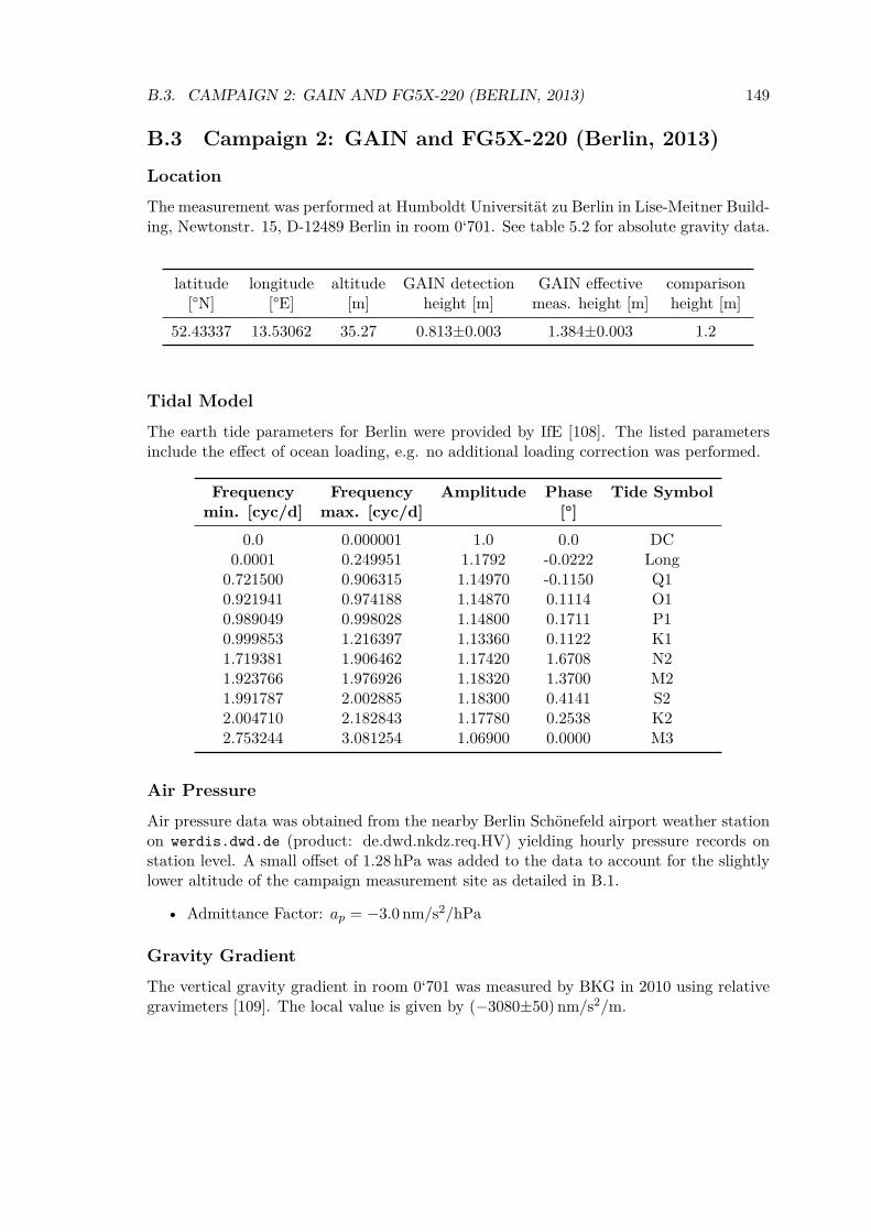
B.3. CAMPAIGN 2: GAIN AND FG5X-220 (BERLIN, 2013) 149
B.3 Campaign 2: GAIN and FG5X-220 (Berlin, 2013)LocationThe measurement was performed at Humboldt Universität zu Berlin in Lise-Meitner Build-ing, Newtonstr. 15, D-12489 Berlin in room 0‘701. See table 5.2 for absolute gravity data.
latitude longitude altitude GAIN detection GAIN effective comparison[°N] [°E] [m] height [m] meas. height [m] height [m]
52.43337 13.53062 35.27 0.813±0.003 1.384±0.003 1.2
Tidal ModelThe earth tide parameters for Berlin were provided by IfE [108]. The listed parametersinclude the effect of ocean loading, e.g. no additional loading correction was performed.
Frequency Frequency Amplitude Phase Tide Symbolmin. [cyc/d] max. [cyc/d] [°]
0.0 0.000001 1.0 0.0 DC0.0001 0.249951 1.1792 -0.0222 Long
0.721500 0.906315 1.14970 -0.1150 Q10.921941 0.974188 1.14870 0.1114 O10.989049 0.998028 1.14800 0.1711 P10.999853 1.216397 1.13360 0.1122 K11.719381 1.906462 1.17420 1.6708 N21.923766 1.976926 1.18320 1.3700 M21.991787 2.002885 1.18300 0.4141 S22.004710 2.182843 1.17780 0.2538 K22.753244 3.081254 1.06900 0.0000 M3
Air PressureAir pressure data was obtained from the nearby Berlin Schönefeld airport weather stationon werdis.dwd.de (product: de.dwd.nkdz.req.HV) yielding hourly pressure records onstation level. A small offset of 1.28 hPa was added to the data to account for the slightlylower altitude of the campaign measurement site as detailed in B.1.
• Admittance Factor: ap = −3.0 nm/s2/hPa
Gravity GradientThe vertical gravity gradient in room 0‘701 was measured by BKG in 2010 using relativegravimeters [109]. The local value is given by (−3080±50) nm/s2/m.
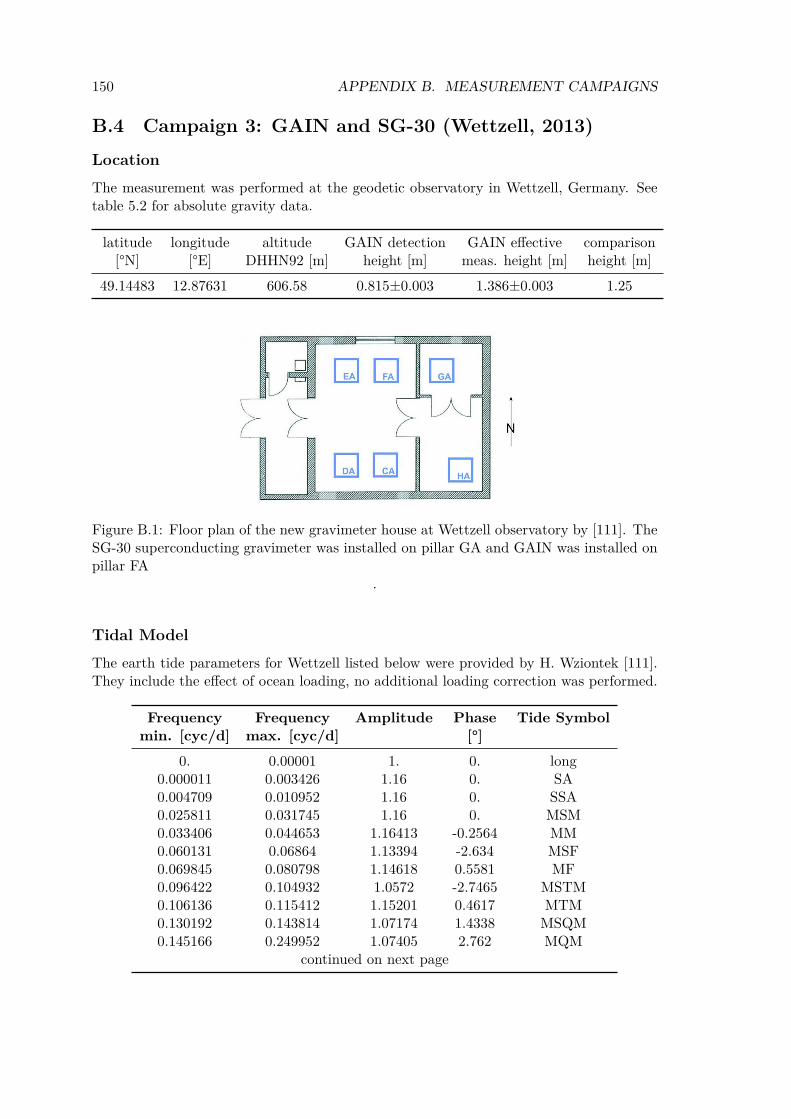
150 APPENDIX B. MEASUREMENT CAMPAIGNS
B.4 Campaign 3: GAIN and SG-30 (Wettzell, 2013)LocationThe measurement was performed at the geodetic observatory in Wettzell, Germany. Seetable 5.2 for absolute gravity data.
latitude longitude altitude GAIN detection GAIN effective comparison[°N] [°E] DHHN92 [m] height [m] meas. height [m] height [m]
49.14483 12.87631 606.58 0.815±0.003 1.386±0.003 1.25
Figure B.1: Floor plan of the new gravimeter house at Wettzell observatory by [111]. TheSG-30 superconducting gravimeter was installed on pillar GA and GAIN was installed onpillar FA
.
Tidal ModelThe earth tide parameters for Wettzell listed below were provided by H. Wziontek [111].They include the effect of ocean loading, no additional loading correction was performed.
Frequency Frequency Amplitude Phase Tide Symbolmin. [cyc/d] max. [cyc/d] [°]
0. 0.00001 1. 0. long0.000011 0.003426 1.16 0. SA0.004709 0.010952 1.16 0. SSA0.025811 0.031745 1.16 0. MSM0.033406 0.044653 1.16413 -0.2564 MM0.060131 0.06864 1.13394 -2.634 MSF0.069845 0.080798 1.14618 0.5581 MF0.096422 0.104932 1.0572 -2.7465 MSTM0.106136 0.115412 1.15201 0.4617 MTM0.130192 0.143814 1.07174 1.4338 MSQM0.145166 0.249952 1.07405 2.762 MQM
continued on next page
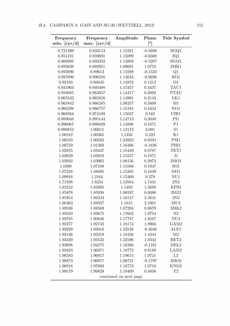
B.4. CAMPAIGN 3: GAIN AND SG-30 (WETTZELL, 2013) 151
Frequency Frequency Amplitude Phase Tide Symbolmin. [cyc/d] max. [cyc/d] [°]
0.721499 0.833113 1.15321 -0.5698 SGQ10.851181 0.859691 1.15099 -0.6368 2Q10.860895 0.892332 1.14803 -0.5287 SGM10.892639 0.892951 1.09091 1.0752 3MK10.893096 0.89613 1.14598 -0.1533 Q10.897806 0.906316 1.14643 -0.0698 RO10.92194 0.93045 1.14852 0.1212 O10.931963 0.940488 1.15457 0.3437 TAU10.958085 0.963857 1.14417 0.3892 NTAU0.965532 0.965828 1.14991 0.3143 LK10.965842 0.966285 1.08257 0.5669 M10.966298 0.966757 1.15184 0.1653 NO10.968564 0.974189 1.15037 0.165 CHI10.989048 0.995144 1.14713 0.3049 PI10.996967 0.998029 1.14896 0.1671 P10.999852 1.00015 1.12173 3.001 S11.00182 1.00365 1.1356 0.223 K11.00533 1.00562 1.24923 0.8594 PSI11.00759 1.01369 1.16486 -0.1826 PHI11.02855 1.03447 1.15449 0.0787 TET11.03629 1.03919 1.15557 0.1071 J11.03932 1.03965 1.08156 0.3972 3MO11.0398 1.07108 1.15508 0.1947 SO11.07258 1.08095 1.15285 0.1639 OO11.09916 1.2164 1.15369 0.379 NU11.71938 1.8234 1.13564 1.7441 3N21.82552 1.85695 1.1492 1.5689 EPS21.85878 1.85938 1.06597 0.0086 3MJ21.85954 1.86243 1.16147 2.3841 2N21.86363 1.89507 1.1615 2.1001 MU21.89536 1.89569 1.07294 0.0679 3MK21.89583 1.89675 1.17662 1.9754 N21.89795 1.90646 1.17787 1.9107 NU21.92377 1.92742 1.18174 1.8966 GAM21.92939 1.93016 1.22538 -0.4048 ALF21.93136 1.93319 1.18426 1.4344 M21.93439 1.93532 1.22596 1.0342 BET21.93698 1.94275 1.16266 -0.1161 DEL21.95823 1.96371 1.18772 0.8189 LAM21.96583 1.96857 1.18615 1.0721 L21.96873 1.96917 1.06721 -0.1797 3MO21.96918 1.97693 1.18773 1.0716 KNO21.99179 1.99829 1.18409 0.4838 T2
continued on next page
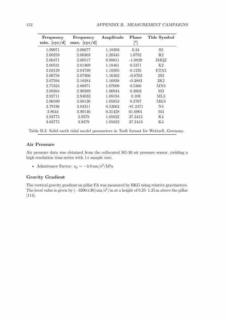
152 APPENDIX B. MEASUREMENT CAMPAIGNS
Frequency Frequency Amplitude Phase Tide Symbolmin. [cyc/d] max. [cyc/d] [°]
1.99971 2.00077 1.18393 0.34 S22.00259 2.00303 1.20345 1.0792 R22.00471 2.00517 0.98011 -1.0829 3MQ22.00531 2.01369 1.18461 0.5371 K22.03129 2.04739 1.18205 0.1235 ETA22.06758 2.07366 1.16462 -0.6703 2S22.07594 2.18284 1.16938 -0.3883 2K22.75324 2.86971 1.07009 0.5366 MN32.89264 2.90389 1.06944 0.3803 M32.92711 2.94033 1.08194 0.109 ML32.96599 3.08126 1.05853 0.2767 MK33.79196 3.83311 0.52662 -81.2471 N43.8644 3.90146 0.31428 61.6901 M43.93775 3.9379 1.05822 37.2413 K43.93775 3.9379 1.05822 37.2413 K4
Table B.3: Solid earth tidal model parameters in Tsoft format for Wettzell, Germany.
Air PressureAir pressure data was obtained from the collocated SG-30 air pressure sensor, yielding ahigh-resolution time-series with 1 s sample rate.
• Admittance Factor: ap = −3.0 nm/s2/hPa
Gravity GradientThe vertical gravity gradient on pillar FA was measured by BKG using relative gravimeters.The local value is given by (−3200±30) nm/s2/m at a height of 0.25–1.25 m above the pillar[114].

B.5. CAMPAIGN 4: GAIN, OSG-054, FG5X-220 (ONSALA, 2015) 153
B.5 Campaign 4: GAIN, OSG-054, FG5X-220 (Onsala, 2015)LocationThe measurement was performed in the gravimeter house at Onsala Space Observatoryin Onsala, Sweden in February 2015. GAIN was located on pillar AA from February 3-8 and on pillar AC from February 8-26. The superconducting gravimeter OSG-054 waslocated about 3 m away on a separate pillar. The FG5X-220 was located on pillar ACfrom February 3-8 and on pillar AA from February 8-12. The absolute gravity comparisonbetween GAIN and the FG5X-220 was performed only for the pillar AC. See table 5.2 forabsolute gravity data.
latitude longitude altitude GAIN detection GAIN effective comparison[°N] [°E] [m] height [m] meas. height [m] height [m]
57.396490 11.925821 8 0.853±0.003 1.423±0.003 1.2
Tidal ModelThe earth tide parameters for Onsala listed below were provided by M. Schilling [70]. Noadditional loading correction was performed.
Frequency Frequency Amplitude Phase Tide Symbolmin. [cyc/d] max. [cyc/d] [°]
0. 0.000001 1. 0. M0S00.000001 0.0024 1.16 0. LONG0.002401 0.00345 2.9101 -24.89 SA0.003451 0.005918 1.11735 -3.54 SSA0.005919 0.00851 1.58376 -9.71 STA0.008511 0.01096 1.77749 22.93 SQA0.010961 0.04466 1.08405 1.17 MM0.044661 0.0808 1.14242 0.01 MF0.080801 0.11542 1.14761 -0.42 MTM0.115421 0.25 1.15726 -6.31 MSQM0.250001 0.870024 1.15095 -0.48 SIG10.870025 0.90632 1.14498 -0.34 Q10.906321 0.94049 1.14826 0.12 O10.940491 0.97419 1.15235 0.22 M10.974191 0.99803 1.15482 0.15 P10.998031 1.00015 1.10669 -2.33 S11.00015 1.00365 1.14098 0.14 K11.00365 1.00563 1.26419 1.04 PSI11.00563 1.01369 1.17893 -0.27 PHI11.01369 1.04481 1.16117 -0.1 J11.04481 1.2164 1.15611 0.01 OO11.2164 1.83797 1.13158 -0.15 3N2
continued on next page
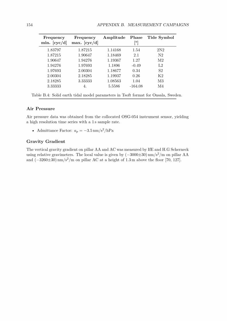
154 APPENDIX B. MEASUREMENT CAMPAIGNS
Frequency Frequency Amplitude Phase Tide Symbolmin. [cyc/d] max. [cyc/d] [°]
1.83797 1.87215 1.14168 1.54 2N21.87215 1.90647 1.18469 2.1 N21.90647 1.94276 1.19367 1.27 M21.94276 1.97693 1.1896 -0.49 L21.97693 2.00304 1.18677 0.34 S22.00304 2.18285 1.19937 0.26 K22.18285 3.33333 1.08563 1.04 M33.33333 4. 5.5586 -164.08 M4
Table B.4: Solid earth tidal model parameters in Tsoft format for Onsala, Sweden.
Air PressureAir pressure data was obtained from the collocated OSG-054 instrument sensor, yieldinga high resolution time series with a 1 s sample rate.
• Admittance Factor: ap = −3.5 nm/s2/hPa
Gravity GradientThe vertical gravity gradient on pillar AA and AC was measured by IfE and H.G Scherneckusing relative gravimeters. The local value is given by (−3000±30) nm/s2/m on pillar AAand (−3260±30) nm/s2/m on pillar AC at a height of 1.3 m above the floor [70, 127].
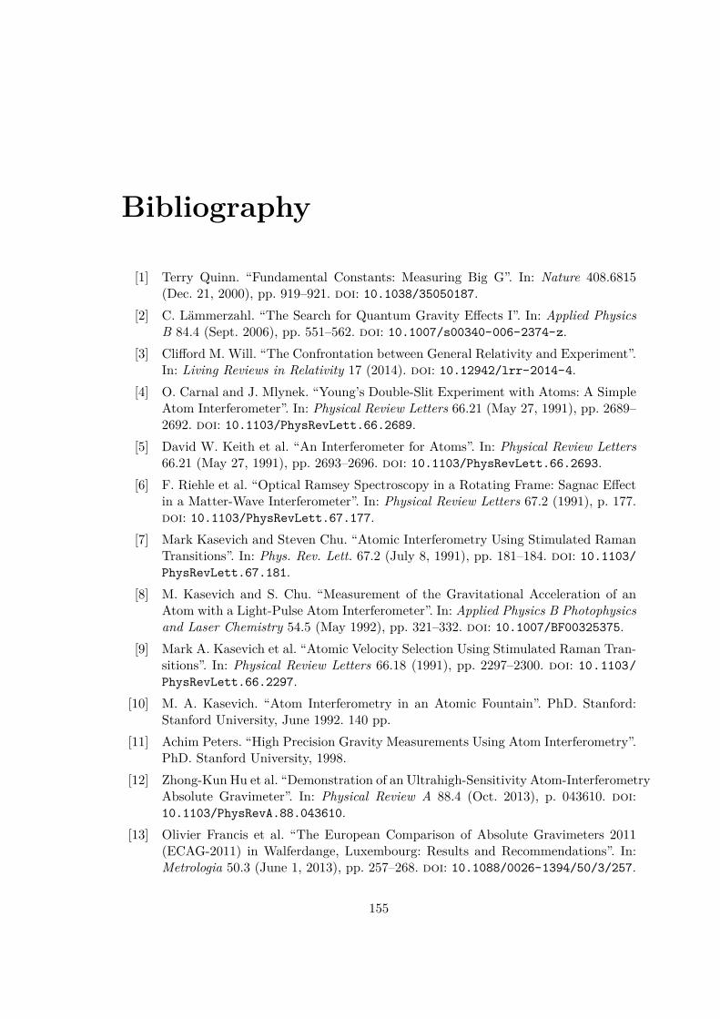
Bibliography
[1] Terry Quinn. “Fundamental Constants: Measuring Big G”. In: Nature 408.6815(Dec. 21, 2000), pp. 919–921. doi: 10.1038/35050187.
[2] C. Lämmerzahl. “The Search for Quantum Gravity Effects I”. In: Applied PhysicsB 84.4 (Sept. 2006), pp. 551–562. doi: 10.1007/s00340-006-2374-z.
[3] Clifford M. Will. “The Confrontation between General Relativity and Experiment”.In: Living Reviews in Relativity 17 (2014). doi: 10.12942/lrr-2014-4.
[4] O. Carnal and J. Mlynek. “Young’s Double-Slit Experiment with Atoms: A SimpleAtom Interferometer”. In: Physical Review Letters 66.21 (May 27, 1991), pp. 2689–2692. doi: 10.1103/PhysRevLett.66.2689.
[5] David W. Keith et al. “An Interferometer for Atoms”. In: Physical Review Letters66.21 (May 27, 1991), pp. 2693–2696. doi: 10.1103/PhysRevLett.66.2693.
[6] F. Riehle et al. “Optical Ramsey Spectroscopy in a Rotating Frame: Sagnac Effectin a Matter-Wave Interferometer”. In: Physical Review Letters 67.2 (1991), p. 177.doi: 10.1103/PhysRevLett.67.177.
[7] Mark Kasevich and Steven Chu. “Atomic Interferometry Using Stimulated RamanTransitions”. In: Phys. Rev. Lett. 67.2 (July 8, 1991), pp. 181–184. doi: 10.1103/PhysRevLett.67.181.
[8] M. Kasevich and S. Chu. “Measurement of the Gravitational Acceleration of anAtom with a Light-Pulse Atom Interferometer”. In: Applied Physics B Photophysicsand Laser Chemistry 54.5 (May 1992), pp. 321–332. doi: 10.1007/BF00325375.
[9] Mark A. Kasevich et al. “Atomic Velocity Selection Using Stimulated Raman Tran-sitions”. In: Physical Review Letters 66.18 (1991), pp. 2297–2300. doi: 10.1103/PhysRevLett.66.2297.
[10] M. A. Kasevich. “Atom Interferometry in an Atomic Fountain”. PhD. Stanford:Stanford University, June 1992. 140 pp.
[11] Achim Peters. “High Precision Gravity Measurements Using Atom Interferometry”.PhD. Stanford University, 1998.
[12] Zhong-Kun Hu et al. “Demonstration of an Ultrahigh-Sensitivity Atom-InterferometryAbsolute Gravimeter”. In: Physical Review A 88.4 (Oct. 2013), p. 043610. doi:10.1103/PhysRevA.88.043610.
[13] Olivier Francis et al. “The European Comparison of Absolute Gravimeters 2011(ECAG-2011) in Walferdange, Luxembourg: Results and Recommendations”. In:Metrologia 50.3 (June 1, 2013), pp. 257–268. doi: 10.1088/0026-1394/50/3/257.
155
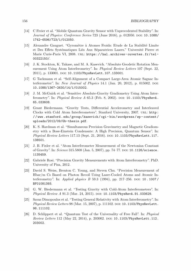
156 BIBLIOGRAPHY
[14] C Freier et al. “Mobile Quantum Gravity Sensor with Unprecedented Stability”. In:Journal of Physics: Conference Series 723 (June 2016), p. 012050. doi: 10.1088/1742-6596/723/1/012050.
[15] Alexandre Gauguet. “Gyromètre à Atomes Froids: Etude de La Stabilité Limiteet Des Effets Systématiques Liés Aux Séparatrices Lasers.” Université Pierre etMarie Curie-Paris VI, 2008. url: https://hal.archives-ouvertes.fr/tel-00322150/.
[16] J. K. Stockton, K. Takase, and M. A. Kasevich. “Absolute Geodetic Rotation Mea-surement Using Atom Interferometry”. In: Physical Review Letters 107 (Sept. 22,2011), p. 133001. doi: 10.1103/PhysRevLett.107.133001.
[17] G Tackmann et al. “Self-Alignment of a Compact Large-Area Atomic Sagnac In-terferometer”. In: New Journal of Physics 14.1 (Jan. 20, 2012), p. 015002. doi:10.1088/1367-2630/14/1/015002.
[18] J. M. McGuirk et al. “Sensitive Absolute-Gravity Gradiometry Using Atom Inter-ferometry”. In: Physical Review A 65.3 (Feb. 8, 2002). doi: 10.1103/PhysRevA.65.033608.
[19] Grant Biedermann. “Gravity Tests, Differential Accelerometry and InterleavedClocks with Cold Atom Interferometers”. Stanford University, 2007. url: http://www.stanford.edu/group/kasevich/cgi- bin/wordpress/wp- content/uploads/2012/09/Gb-thesis.pdf.
[20] K. S. Hardman et al. “Simultaneous Precision Gravimetry and Magnetic Gradiom-etry with a Bose-Einstein Condensate: A High Precision, Quantum Sensor”. In:Physical Review Letters 117.13 (Sept. 21, 2016). doi: 10.1103/PhysRevLett.117.138501.
[21] J. B. Fixler et al. “Atom Interferometer Measurement of the Newtonian Constantof Gravity”. In: Science 315.5808 (Jan. 5, 2007), pp. 74–77. doi: 10.1126/science.1135459.
[22] Gabriele Rosi. “Precision Gravity Measurements with Atom Interferometry”. PhD.University of Pisa, 2012.
[23] David S. Weiss, Brenton C. Young, and Steven Chu. “Precision Measurement ofHbar/m Cs Based on Photon Recoil Using Laser-Cooled Atoms and Atomic In-terferometry”. In: Applied physics B 59.3 (1994), pp. 217–256. doi: 10 . 1007 /BF01081393.
[24] G. W. Biedermann et al. “Testing Gravity with Cold-Atom Interferometers”. In:Physical Review A 91.3 (Mar. 24, 2015). doi: 10.1103/PhysRevA.91.033629.
[25] Savas Dimopoulos et al. “Testing General Relativity with Atom Interferometry”. In:Physical Review Letters 98 (Mar. 15, 2007), p. 111102. doi: 10.1103/PhysRevLett.98.111102.
[26] D. Schlippert et al. “Quantum Test of the Universality of Free Fall”. In: PhysicalReview Letters 112 (May 22, 2014), p. 203002. doi: 10.1103/PhysRevLett.112.203002.
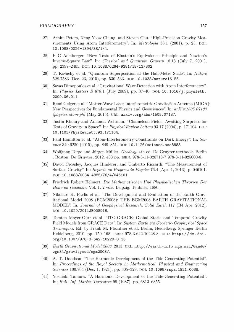
BIBLIOGRAPHY 157
[27] Achim Peters, Keng Yeow Chung, and Steven Chu. “High-Precision Gravity Mea-surements Using Atom Interferometry”. In: Metrologia 38.1 (2001), p. 25. doi:10.1088/0026-1394/38/1/4.
[28] E G Adelberger. “New Tests of Einstein’s Equivalence Principle and Newton’sInverse-Square Law”. In: Classical and Quantum Gravity 18.13 (July 7, 2001),pp. 2397–2405. doi: 10.1088/0264-9381/18/13/302.
[29] T. Kovachy et al. “Quantum Superposition at the Half-Metre Scale”. In: Nature528.7583 (Dec. 23, 2015), pp. 530–533. doi: 10.1038/nature16155.
[30] Savas Dimopoulos et al. “Gravitational Wave Detection with Atom Interferometry”.In: Physics Letters B 678.1 (July 2009), pp. 37–40. doi: 10.1016/j.physletb.2009.06.011.
[31] Remi Geiger et al. “Matter-Wave Laser Interferometric Gravitation Antenna (MIGA):New Perspectives for Fundamental Physics and Geosciences”. In: arXiv:1505.07137[physics.atom-ph] (May 2015). url: arxiv.org/abs/1505.07137.
[32] Justin Khoury and Amanda Weltman. “Chameleon Fields: Awaiting Surprises forTests of Gravity in Space”. In: Physical Review Letters 93.17 (2004), p. 171104. doi:10.1103/PhysRevLett.93.171104.
[33] Paul Hamilton et al. “Atom-Interferometry Constraints on Dark Energy”. In: Sci-ence 349.6250 (2015), pp. 849–851. doi: 10.1126/science.aaa8883.
[34] Wolfgang Torge and Jürgen Müller. Geodesy. 4th ed. De Gruyter textbook. Berlin; Boston: De Gruyter, 2012. 433 pp. isbn: 978-3-11-020718-7 978-3-11-025000-8.
[35] David Crossley, Jacques Hinderer, and Umberto Riccardi. “The Measurement ofSurface Gravity”. In: Reports on Progress in Physics 76.4 (Apr. 1, 2013), p. 046101.doi: 10.1088/0034-4885/76/4/046101.
[36] Friedrich Robert Helmert. Die Mathematischen Und Physikalischen Theorien DerHöheren Geodäsie. Vol. 1. 2 vols. Leipzig: Teubner, 1880.
[37] Nikolaos K. Pavlis et al. “The Development and Evaluation of the Earth Grav-itational Model 2008 (EGM2008): THE EGM2008 EARTH GRAVITATIONALMODEL”. In: Journal of Geophysical Research: Solid Earth 117 (B4 Apr. 2012).doi: 10.1029/2011JB008916.
[38] Torsten Mayer-Gürr et al. “ITG-GRACE: Global Static and Temporal GravityField Models from GRACE Data”. In: System Earth via Geodetic-Geophysical SpaceTechniques. Ed. by Frank M. Flechtner et al. Berlin, Heidelberg: Springer BerlinHeidelberg, 2010, pp. 159–168. isbn: 978-3-642-10228-8. url: http://dx.doi.org/10.1007/978-3-642-10228-8_13.
[39] Earth Gravitational Model 2008. 2013. url: http://earth-info.nga.mil/GandG/wgs84/gravitymod/egm2008/.
[40] A. T. Doodson. “The Harmonic Development of the Tide-Generating Potential”.In: Proceedings of the Royal Society A: Mathematical, Physical and EngineeringSciences 100.704 (Dec. 1, 1921), pp. 305–329. doi: 10.1098/rspa.1921.0088.
[41] Yoshiaki Tamura. “A Harmonic Development of the Tide-Generating Potential”.In: Bull. Inf. Marées Terrestres 99 (1987), pp. 6813–6855.
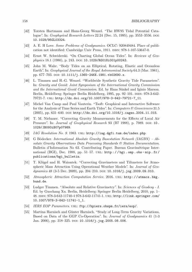
158 BIBLIOGRAPHY
[42] Torsten Hartmann and Hans-Georg Wenzel. “The HW95 Tidal Potential Cata-logue”. In: Geophysical Research Letters 22.24 (Dec. 15, 1995), pp. 3553–3556. doi:10.1029/95GL03324.
[43] A. E. H Love. Some Problems of Geodynamics. OCLC: 920849484. Place of publi-cation not identified: Cambridge Univ Press, 1911. isbn: 978-1-107-53647-0.
[44] Ernst W. Schwiderski. “On Charting Global Ocean Tides”. In: Reviews of Geo-physics 18.1 (1980), p. 243. doi: 10.1029/RG018i001p00243.
[45] John M. Wahr. “Body Tides on an Elliptical, Rotating, Elastic and OceanlessEarth”. In: Geophysical Journal of the Royal Astronomical Society 64.3 (Mar. 1981),pp. 677–703. doi: 10.1111/j.1365-246X.1981.tb02690.x.
[46] L. Timmen and H.-G. Wenzel. “Worldwide Synthetic Gravity Tide Parameters”.In: Gravity and Geoid: Joint Symposium of the International Gravity Commissionand the International Geoid Commission. Ed. by Hans Sünkel and Iginio Marson.Berlin, Heidelberg: Springer Berlin Heidelberg, 1995, pp. 92–101. isbn: 978-3-642-79721-7. url: http://dx.doi.org/10.1007/978-3-642-79721-7_11.
[47] Michel Van Camp and Paul Vauterin. “Tsoft: Graphical and Interactive Softwarefor the Analysis of Time Series and Earth Tides”. In: Computers & Geosciences 31.5(2005), pp. 631–640. doi: http://dx.doi.org/10.1016/j.cageo.2004.11.015.
[48] T. M. Niebauer. “Correcting Gravity Measurements for the Effects of Local AirPressure”. In: Journal of Geophysical Research 93 (B7 1988), p. 7989. doi: 10.1029/JB093iB07p07989.
[49] IAG Resolution No. 9. 1983. url: http://iag.dgfi.tum.de/index.php.[50] G Bödecker. International Absolute Gravity Basestation Network (IAGBN) – Ab-
solute Gravity Observations Data Processing Standards & Station Documentation.Bulletin d’Information No 63. Contributing Paper. Bureau Gravimétrique Inter-national (BGI), Dec. 1988, pp. 51–57. url: http : / / bgi . omp . obs - mip . fr /publications/bgi_bulletin.
[51] T. Klügel and H. Wziontek. “Correcting Gravimeters and Tiltmeters for Atmo-spheric Mass Attraction Using Operational Weather Models”. In: Journal of Geo-dynamics 48 (3-5 Dec. 2009), pp. 204–210. doi: 10.1016/j.jog.2009.09.010.
[52] Atmospheric Attraction Computation Service. 2016. url: http://atmacs.bkg.bund.de.
[53] Ludger Timmen. “Absolute and Relative Gravimetry”. In: Sciences of Geodesy - I.Ed. by Guochang Xu. Berlin, Heidelberg: Springer Berlin Heidelberg, 2010, pp. 1–48. isbn: 978-3-642-11740-4 978-3-642-11741-1. url: http://link.springer.com/10.1007/978-3-642-11741-1_1.
[54] IERS EOP Parameters. url: ftp://hpiers.obspm.fr/iers/eop/.[55] Martina Harnisch and Günter Harnisch. “Study of Long-Term Gravity Variations,
Based on Data of the GGP Co-Operation”. In: Journal of Geodynamics 41 (1-3Jan. 2006), pp. 318–325. doi: 10.1016/j.jog.2005.08.006.

BIBLIOGRAPHY 159
[56] M. Hauth et al. “Atom Interferometry for Absolute Measurements of Local Grav-ity”. In: Proc. of the Int. School of Physics ”Enrico Fermi”, Course 188, Edited byTino G. M. and Kasevich M. A. SIF, Bologna and IOS Press, Amsterdam, May2014, pp. 557–586. doi: 10.3254/978-1-61499-448-0-557.
[57] L. A. Krieg and Ohio State University. Department of Geodetic Science. Mathe-matical Modelling of the Behaviour of the Lacoste and Romberg ”G” Gravity Meterfor Use in Gravity Network Adjustments and Data Analyses. Columbus: [s.n.], 1981.
[58] Manuel Schilling and Olga Gitlein. “Accuracy Estimation of the IfE GravimetersMicro-g LaCoste gPhone-98 and ZLS Burris Gravity Meter B-64”. In: Berlin, Hei-delberg: Springer Berlin Heidelberg, 2015. url: http://link.springer.com/10.1007/1345_2015_29.
[59] J. Hinderer, D. Crossley, and R.J. Warburton. “Superconducting Gravimetry”. In:Treatise on Geophysics. Elsevier, 2015, pp. 59–115. isbn: 978-0-444-53803-1. url:http://dx.doi.org/10.1016/B978-0-444-53802-4.00062-2.
[60] John M. Goodkind. “The Superconducting Gravimeter”. In: Review of ScientificInstruments 70.11 (1999), p. 4131. doi: 10.1063/1.1150092.
[61] GWR Instruments. 2015. url: http://www.gwrinstruments.com.[62] William M. Telford, Lloyd P. Geldart, and Robert E. Sheriff. Applied Geophysics.
2. ed., transferred to digital printing. OCLC: 552143005. Cambridge: CambridgeUniv. Press, 2004. 770 pp. isbn: 978-0-521-33938-4 978-0-521-32693-3.
[63] J E Faller and I Marson. “Ballistic Methods of Measuring g - the Direct Free-Falland Symmetrical Rise-and-Fall Methods Compared”. In: Metrologia 25.1 (Jan. 1,1988), pp. 49–55. doi: 10.1088/0026-1394/25/1/008.
[64] T. M. Niebauer et al. “A New Generation of Absolute Gravimeters”. In: Metrologia32.3 (1995), p. 159. doi: 10.1088/0026-1394/32/3/004.
[65] Olivier Francis et al. “CCM.G-K2 Key Comparison”. In: Metrologia 52 (1A Jan. 1,2015), p. 07009. doi: 10.1088/0026-1394/52/1A/07009.
[66] T M Niebauer et al. “The Self-Attraction Correction for the FG5X Absolute GravityMeter”. In: Metrologia 50.1 (Feb. 1, 2013), pp. 1–8. doi: 10.1088/0026-1394/50/1/1.
[67] James E. Faller. “Super Spring”. In: The Journal of the Acoustical Society of Amer-ica 68.6 (1980), p. 1900. doi: 10.1121/1.385186.
[68] Robert Lee. Rinker. “Super Spring : A New Type of Low-Frequency VibrationIsolator”. PhD. University of Colorado, 1983.
[69] Manuel Schilling and Ludger Timmen. “Traceability of the Hannover FG5X-220to the SI Units”. In: Berlin, Heidelberg: Springer Berlin Heidelberg, 2016. url:http://link.springer.com/10.1007/1345_2016_226.
[70] Manuel Schilling. Private communication. 2015.[71] Jürgen Müller et al. “A Land Uplift Model in Fennoscandia Combining GRACE
and Absolute Gravimetry Data”. In: Physics and Chemistry of the Earth, PartsA/B/C 53-54 (Jan. 2012), pp. 54–60. doi: 10.1016/j.pce.2010.12.006.

160 BIBLIOGRAPHY
[72] Jeffrey Kennedy et al. “Gravity‐Measured Water Storage Change and SubsurfaceHydraulic Properties at a Managed Recharge Facility in Tucson, USA”. In: Envi-ronment and Engineering Geophysical Society, Jan. 2012, pp. 58–58. doi: 10.4133/1.4721694.
[73] Andreas Guntner et al. “Monitoring Water Storage Variations with a Supercon-ducting Gravimeter in a Field Enclosure”. In: EGU General Assembly 2016. Vienna,Apr. 2016, p. 5173.
[74] Patrick Cheinet. “Conception et Réalisation d’un Gravimètre à Atomes Froids”.Université Pierre et Marie Curie-Paris VI, 2006. url: http://hal.upmc.fr/tel-00070861/.
[75] MuQuans. 2014. url: http://www.muquans.com/.[76] AoSense. 2016. url: http://aosense.com.[77] AtomSensors. 2016. url: http://www.atomsensors.com/.[78] Paul R. Berman, ed. Atom Interferometry. San Diego: Academic Press, 1997.
478 pp. isbn: 978-0-12-092460-8.[79] Daniel A. Steck. Quantum and Atom Optics. revision 0.5.12. Eugene, Oregon, 2011.
url: http://steck.us/teaching.[80] Matthias Hauth. “A Mobile, High-Precision Atom-Interferometer and Its Applica-
tion to Gravity Observations”. PhD. Berlin: Humboldt Universität zu Berlin, 2015.[81] Harold J. Metcalf and Peter Van der Straten. Laser Cooling and Trapping. Graduate
texts in contemporary physics. New York: Springer, 1999. 323 pp. isbn: 0-387-98747-9 0-387-98728-2.
[82] Malte Schmidt. “A Mobile High-Precision Gravimeter Based on Atom Interferom-etry”. PhD. Berlin: Humboldt Universität zu Berlin, 2011. url: http://edoc.hu-berlin.de/dissertationen/schmidt-malte-2011-11-02.
[83] J. Le Gouët. “Etude Des Performances d’un Gravimetre Atomique Absolu : Sensi-bilite Limite et Exactitude Preliminaire”. PhD. University Paris-Sud 11, 2008. url:https://tel.archives-ouvertes.fr/tel-00311422v4.
[84] Pippa Storey and Claude Cohen-Tannoudji. “The Feynman Path Integral Approachto Atomic Interferometry. A Tutorial”. In: J. Phys. II France 4.11 (1994), pp. 1999–2027. doi: 10.1051/jp2:1994103.
[85] Kai Bongs, R. Launay, and Mark A Kasevich. “High-Order Inertial Phase Shiftsfor Time-Domain Atom Interferometers”. In: Applied Physics B 84.4 (Aug. 2006),pp. 599–602. doi: 10.1007/s00340-006-2397-5.
[86] Jason M. Hogan, David M S Johnson, and Mark A Kasevich. “Light-Pulse AtomInterferometry”. In: Proceedings of the International School of Physics Enrico FermiCourse CLXVIII on Atom Optics and Space Physics. Ed. by E. Arimondo et al.Oxford: IOS Press, June 2007, pp. 411–447. doi: 10.3254/978-1-58603-990-5-411.
[87] Ch J. Bordé. “Atomic Clocks and Inertial Sensors”. In: Metrologia 39.5 (2002),p. 435. doi: 10.1088/0026-1394/39/5/5.
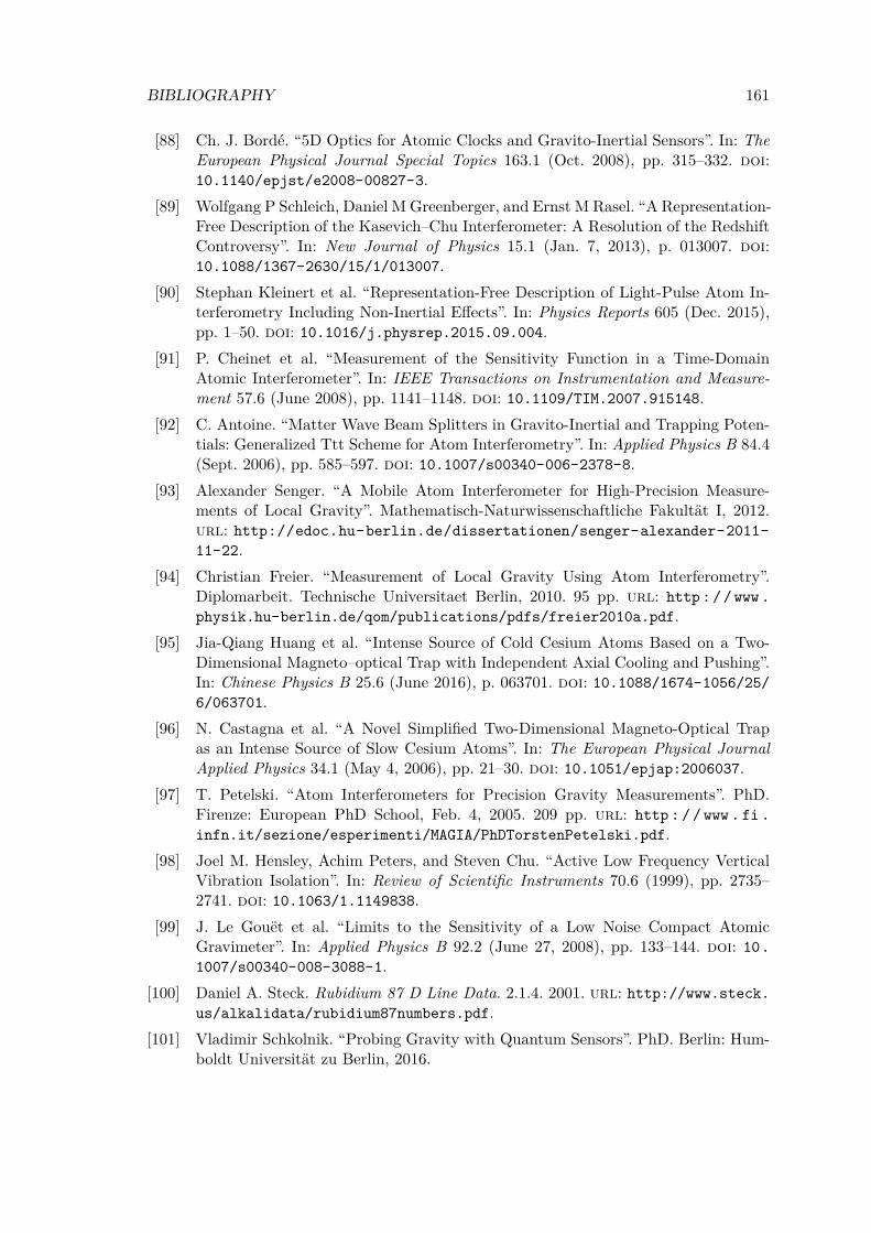
BIBLIOGRAPHY 161
[88] Ch. J. Bordé. “5D Optics for Atomic Clocks and Gravito-Inertial Sensors”. In: TheEuropean Physical Journal Special Topics 163.1 (Oct. 2008), pp. 315–332. doi:10.1140/epjst/e2008-00827-3.
[89] Wolfgang P Schleich, Daniel M Greenberger, and Ernst M Rasel. “A Representation-Free Description of the Kasevich–Chu Interferometer: A Resolution of the RedshiftControversy”. In: New Journal of Physics 15.1 (Jan. 7, 2013), p. 013007. doi:10.1088/1367-2630/15/1/013007.
[90] Stephan Kleinert et al. “Representation-Free Description of Light-Pulse Atom In-terferometry Including Non-Inertial Effects”. In: Physics Reports 605 (Dec. 2015),pp. 1–50. doi: 10.1016/j.physrep.2015.09.004.
[91] P. Cheinet et al. “Measurement of the Sensitivity Function in a Time-DomainAtomic Interferometer”. In: IEEE Transactions on Instrumentation and Measure-ment 57.6 (June 2008), pp. 1141–1148. doi: 10.1109/TIM.2007.915148.
[92] C. Antoine. “Matter Wave Beam Splitters in Gravito-Inertial and Trapping Poten-tials: Generalized Ttt Scheme for Atom Interferometry”. In: Applied Physics B 84.4(Sept. 2006), pp. 585–597. doi: 10.1007/s00340-006-2378-8.
[93] Alexander Senger. “A Mobile Atom Interferometer for High-Precision Measure-ments of Local Gravity”. Mathematisch-Naturwissenschaftliche Fakultät I, 2012.url: http://edoc.hu-berlin.de/dissertationen/senger-alexander-2011-11-22.
[94] Christian Freier. “Measurement of Local Gravity Using Atom Interferometry”.Diplomarbeit. Technische Universitaet Berlin, 2010. 95 pp. url: http://www.physik.hu-berlin.de/qom/publications/pdfs/freier2010a.pdf.
[95] Jia-Qiang Huang et al. “Intense Source of Cold Cesium Atoms Based on a Two-Dimensional Magneto–optical Trap with Independent Axial Cooling and Pushing”.In: Chinese Physics B 25.6 (June 2016), p. 063701. doi: 10.1088/1674-1056/25/6/063701.
[96] N. Castagna et al. “A Novel Simplified Two-Dimensional Magneto-Optical Trapas an Intense Source of Slow Cesium Atoms”. In: The European Physical JournalApplied Physics 34.1 (May 4, 2006), pp. 21–30. doi: 10.1051/epjap:2006037.
[97] T. Petelski. “Atom Interferometers for Precision Gravity Measurements”. PhD.Firenze: European PhD School, Feb. 4, 2005. 209 pp. url: http : / / www . fi .infn.it/sezione/esperimenti/MAGIA/PhDTorstenPetelski.pdf.
[98] Joel M. Hensley, Achim Peters, and Steven Chu. “Active Low Frequency VerticalVibration Isolation”. In: Review of Scientific Instruments 70.6 (1999), pp. 2735–2741. doi: 10.1063/1.1149838.
[99] J. Le Gouët et al. “Limits to the Sensitivity of a Low Noise Compact AtomicGravimeter”. In: Applied Physics B 92.2 (June 27, 2008), pp. 133–144. doi: 10.1007/s00340-008-3088-1.
[100] Daniel A. Steck. Rubidium 87 D Line Data. 2.1.4. 2001. url: http://www.steck.us/alkalidata/rubidium87numbers.pdf.
[101] Vladimir Schkolnik. “Probing Gravity with Quantum Sensors”. PhD. Berlin: Hum-boldt Universität zu Berlin, 2016.
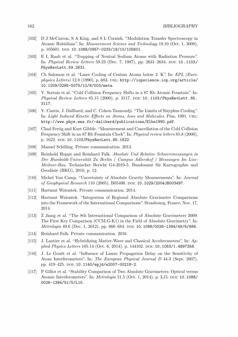
162 BIBLIOGRAPHY
[102] D J McCarron, S A King, and S L Cornish. “Modulation Transfer Spectroscopy inAtomic Rubidium”. In: Measurement Science and Technology 19.10 (Oct. 1, 2008),p. 105601. doi: 10.1088/0957-0233/19/10/105601.
[103] E L Raab et al. “Trapping of Neutral Sodium Atoms with Radiation Pressure”.In: Physical Review Letters 59.23 (Dec. 7, 1987), pp. 2631–2634. doi: 10.1103/PhysRevLett.59.2631.
[104] Ch Salomon et al. “Laser Cooling of Cesium Atoms below 3 K”. In: EPL (Euro-physics Letters) 12.8 (1990), p. 683. url: http://iopscience.iop.org/article/10.1209/0295-5075/12/8/003/meta.
[105] Y. Sortais et al. “Cold Collision Frequency Shifts in a 87 Rb Atomic Fountain”. In:Physical Review Letters 85.15 (2000), p. 3117. doi: 10.1103/PhysRevLett.85.3117.
[106] Y. Castin, J. Dallbard, and C. Cohen-Tannoudji. “The Limits of Sisyphus Cooling”.In: Light Induced Kinetic Effects on Atoms, Ions and Molecules. Pisa, 1991. url:http://www.phys.ens.fr/~dalibard/publications/Elba1990.pdf.
[107] Chad Fertig and Kurt Gibble. “Measurement and Cancellation of the Cold CollisionFrequency Shift in an 87 Rb Fountain Clock”. In: Physical review letters 85.8 (2000),p. 1622. doi: 10.1103/PhysRevLett.85.1622.
[108] Manuel Schilling. Private communication. 2013.[109] Reinhold Hoppe and Reinhard Falk. Absolute Und Relative Schweremessungen in
Der Humboldt-Universität Zu Berlin ( Campus Adlershof ) Messungen Im Lise-Meitner-Bau. Technischer Bericht G4-2010-5. Bundesamt für Kartographie undGeodäsie (BKG), 2010, p. 12.
[110] Michel Van Camp. “Uncertainty of Absolute Gravity Measurements”. In: Journalof Geophysical Research 110 (2005), B05406. doi: 10.1029/2004JB003497.
[111] Hartmut Wziontek. Private communication. 2014.[112] Hartmut Wziontek. “Integration of Regional Absolute Gravimeter Comparisons
into the Framework of the International Comparisons”. Strasbourg, France, Nov. 17,2014.
[113] Z Jiang et al. “The 8th International Comparison of Absolute Gravimeters 2009:The First Key Comparison (CCM.G-K1) in the Field of Absolute Gravimetry”. In:Metrologia 49.6 (Dec. 1, 2012), pp. 666–684. doi: 10.1088/0026-1394/49/6/666.
[114] Reinhard Falk. Private communication. 2016.[115] J. Lautier et al. “Hybridizing Matter-Wave and Classical Accelerometers”. In: Ap-
plied Physics Letters 105.14 (Oct. 6, 2014), p. 144102. doi: 10.1063/1.4897358.[116] J. Le Gouët et al. “Influence of Lasers Propagation Delay on the Sensitivity of
Atom Interferometers”. In: The European Physical Journal D 44.3 (Sept. 2007),pp. 419–425. doi: 10.1140/epjd/e2007-00218-2.
[117] P Gillot et al. “Stability Comparison of Two Absolute Gravimeters: Optical versusAtomic Interferometers”. In: Metrologia 51.5 (Oct. 1, 2014), p. L15. doi: 10.1088/0026-1394/51/5/L15.
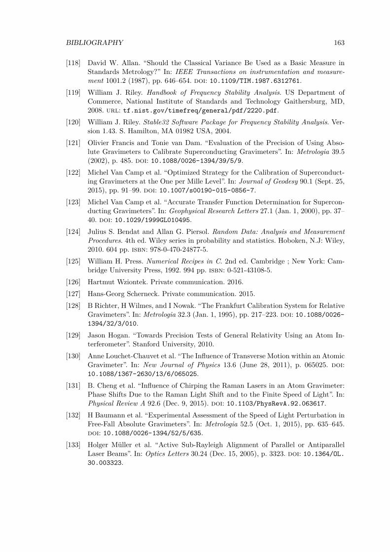
BIBLIOGRAPHY 163
[118] David W. Allan. “Should the Classical Variance Be Used as a Basic Measure inStandards Metrology?” In: IEEE Transactions on instrumentation and measure-ment 1001.2 (1987), pp. 646–654. doi: 10.1109/TIM.1987.6312761.
[119] William J. Riley. Handbook of Frequency Stability Analysis. US Department ofCommerce, National Institute of Standards and Technology Gaithersburg, MD,2008. url: tf.nist.gov/timefreq/general/pdf/2220.pdf.
[120] William J. Riley. Stable32 Software Package for Frequency Stability Analysis. Ver-sion 1.43. S. Hamilton, MA 01982 USA, 2004.
[121] Olivier Francis and Tonie van Dam. “Evaluation of the Precision of Using Abso-lute Gravimeters to Calibrate Superconducting Gravimeters”. In: Metrologia 39.5(2002), p. 485. doi: 10.1088/0026-1394/39/5/9.
[122] Michel Van Camp et al. “Optimized Strategy for the Calibration of Superconduct-ing Gravimeters at the One per Mille Level”. In: Journal of Geodesy 90.1 (Sept. 25,2015), pp. 91–99. doi: 10.1007/s00190-015-0856-7.
[123] Michel Van Camp et al. “Accurate Transfer Function Determination for Supercon-ducting Gravimeters”. In: Geophysical Research Letters 27.1 (Jan. 1, 2000), pp. 37–40. doi: 10.1029/1999GL010495.
[124] Julius S. Bendat and Allan G. Piersol. Random Data: Analysis and MeasurementProcedures. 4th ed. Wiley series in probability and statistics. Hoboken, N.J: Wiley,2010. 604 pp. isbn: 978-0-470-24877-5.
[125] William H. Press. Numerical Recipes in C. 2nd ed. Cambridge ; New York: Cam-bridge University Press, 1992. 994 pp. isbn: 0-521-43108-5.
[126] Hartmut Wziontek. Private communication. 2016.[127] Hans-Georg Scherneck. Private communication. 2015.[128] B Richter, H Wilmes, and I Nowak. “The Frankfurt Calibration System for Relative
Gravimeters”. In: Metrologia 32.3 (Jan. 1, 1995), pp. 217–223. doi: 10.1088/0026-1394/32/3/010.
[129] Jason Hogan. “Towards Precision Tests of General Relativity Using an Atom In-terferometer”. Stanford University, 2010.
[130] Anne Louchet-Chauvet et al. “The Influence of Transverse Motion within an AtomicGravimeter”. In: New Journal of Physics 13.6 (June 28, 2011), p. 065025. doi:10.1088/1367-2630/13/6/065025.
[131] B. Cheng et al. “Influence of Chirping the Raman Lasers in an Atom Gravimeter:Phase Shifts Due to the Raman Light Shift and to the Finite Speed of Light”. In:Physical Review A 92.6 (Dec. 9, 2015). doi: 10.1103/PhysRevA.92.063617.
[132] H Baumann et al. “Experimental Assessment of the Speed of Light Perturbation inFree-Fall Absolute Gravimeters”. In: Metrologia 52.5 (Oct. 1, 2015), pp. 635–645.doi: 10.1088/0026-1394/52/5/635.
[133] Holger Müller et al. “Active Sub-Rayleigh Alignment of Parallel or AntiparallelLaser Beams”. In: Optics Letters 30.24 (Dec. 15, 2005), p. 3323. doi: 10.1364/OL.30.003323.
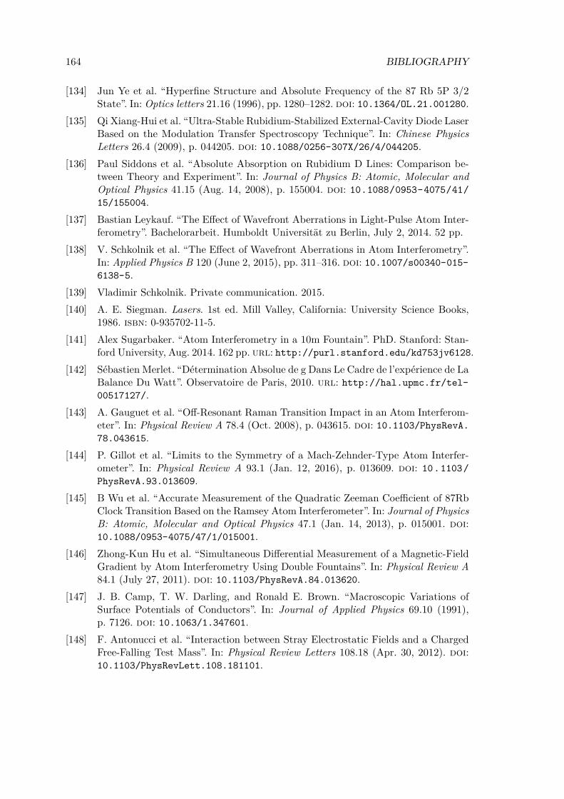
164 BIBLIOGRAPHY
[134] Jun Ye et al. “Hyperfine Structure and Absolute Frequency of the 87 Rb 5P 3/2State”. In: Optics letters 21.16 (1996), pp. 1280–1282. doi: 10.1364/OL.21.001280.
[135] Qi Xiang-Hui et al. “Ultra-Stable Rubidium-Stabilized External-Cavity Diode LaserBased on the Modulation Transfer Spectroscopy Technique”. In: Chinese PhysicsLetters 26.4 (2009), p. 044205. doi: 10.1088/0256-307X/26/4/044205.
[136] Paul Siddons et al. “Absolute Absorption on Rubidium D Lines: Comparison be-tween Theory and Experiment”. In: Journal of Physics B: Atomic, Molecular andOptical Physics 41.15 (Aug. 14, 2008), p. 155004. doi: 10.1088/0953-4075/41/15/155004.
[137] Bastian Leykauf. “The Effect of Wavefront Aberrations in Light-Pulse Atom Inter-ferometry”. Bachelorarbeit. Humboldt Universität zu Berlin, July 2, 2014. 52 pp.
[138] V. Schkolnik et al. “The Effect of Wavefront Aberrations in Atom Interferometry”.In: Applied Physics B 120 (June 2, 2015), pp. 311–316. doi: 10.1007/s00340-015-6138-5.
[139] Vladimir Schkolnik. Private communication. 2015.[140] A. E. Siegman. Lasers. 1st ed. Mill Valley, California: University Science Books,
1986. isbn: 0-935702-11-5.[141] Alex Sugarbaker. “Atom Interferometry in a 10m Fountain”. PhD. Stanford: Stan-
ford University, Aug. 2014. 162 pp. url: http://purl.stanford.edu/kd753jv6128.[142] Sébastien Merlet. “Détermination Absolue de g Dans Le Cadre de l’expérience de La
Balance Du Watt”. Observatoire de Paris, 2010. url: http://hal.upmc.fr/tel-00517127/.
[143] A. Gauguet et al. “Off-Resonant Raman Transition Impact in an Atom Interferom-eter”. In: Physical Review A 78.4 (Oct. 2008), p. 043615. doi: 10.1103/PhysRevA.78.043615.
[144] P. Gillot et al. “Limits to the Symmetry of a Mach-Zehnder-Type Atom Interfer-ometer”. In: Physical Review A 93.1 (Jan. 12, 2016), p. 013609. doi: 10.1103/PhysRevA.93.013609.
[145] B Wu et al. “Accurate Measurement of the Quadratic Zeeman Coefficient of 87RbClock Transition Based on the Ramsey Atom Interferometer”. In: Journal of PhysicsB: Atomic, Molecular and Optical Physics 47.1 (Jan. 14, 2013), p. 015001. doi:10.1088/0953-4075/47/1/015001.
[146] Zhong-Kun Hu et al. “Simultaneous Differential Measurement of a Magnetic-FieldGradient by Atom Interferometry Using Double Fountains”. In: Physical Review A84.1 (July 27, 2011). doi: 10.1103/PhysRevA.84.013620.
[147] J. B. Camp, T. W. Darling, and Ronald E. Brown. “Macroscopic Variations ofSurface Potentials of Conductors”. In: Journal of Applied Physics 69.10 (1991),p. 7126. doi: 10.1063/1.347601.
[148] F. Antonucci et al. “Interaction between Stray Electrostatic Fields and a ChargedFree-Falling Test Mass”. In: Physical Review Letters 108.18 (Apr. 30, 2012). doi:10.1103/PhysRevLett.108.181101.
BIBLIOGRAPHY 165
[149] J. D. Carter and J. D. D. Martin. “Energy Shifts of Rydberg Atoms Due to PatchFields near Metal Surfaces”. In: Physical Review A 83.3 (Mar. 7, 2011). doi: 10.1103/PhysRevA.83.032902.
[150] Kurt Gibble and Steven Chu. “Laser-Cooled Cs Frequency Standard and a Measure-ment of the Frequency Shift Due to Ultracold Collisions”. In: Physical Review Let-ters 70.12 (Mar. 22, 1993), pp. 1771–1774. doi: 10.1103/PhysRevLett.70.1771.
[151] I. Dutta et al. “Continuous Cold-Atom Inertial Sensor with 1 Nrad / Sec Rota-tion Stability”. In: Physical Review Letters 116.18 (May 6, 2016). doi: 10.1103/PhysRevLett.116.183003.
[152] Nassim Zahzam et al. “New Advances in the Field of Cold Atom Interferometersfor Onboard Gravimetry”. Presentation. St. Petersburg, 2016. url: http://www.elektropribor.spb.ru/tgsmm2016/eginf.
[153] V. Menoret et al. “Quantitative Analysis of a Transportable Matter-Wave Gravime-ter”. Presentation. St. Petersburg, 2016.
[154] Alexis Bonnin. “Simultaneous Interferometry with Two Atomic Species 87Rb/85Rband Applications to Inertial Measurements”. PhD. Université Paris-Saclay, Nov.2015. url: https://tel.archives-ouvertes.fr/tel-01272542.

166 BIBLIOGRAPHY
List of Figures
1.1 Mach-Zehnder Atom Interferometer space-time diagram. . . . . . . . . . . . 131.2 Map of world-wide free-air gravity anomalies. . . . . . . . . . . . . . . . . . 151.3 Basic tidal effect caused by celestial bodies. . . . . . . . . . . . . . . . . . . 161.4 Preview of tidal gravity changes measured by GAIN. . . . . . . . . . . . . . 171.5 Relative spring gravimeter operating principle. . . . . . . . . . . . . . . . . 211.6 Relative superconducting gravimeter operating principle. . . . . . . . . . . . 231.7 Absolute falling corner-cube gravimeter operating principle. . . . . . . . . . 24
2.1 Three-Level system and stimulated Raman transitions. . . . . . . . . . . . . 302.2 Realistic Mach-Zehnder atom interferometer space-time diagram. . . . . . . 352.3 Sensitivity function g(t) . . . . . . . . . . . . . . . . . . . . . . . . . . . . . 382.4 Interferometer transfer function to Raman phase noise (normalized). . . . . 392.5 Interferometer transfer function to mirror vibrations. . . . . . . . . . . . . . 40
3.1 Photograph of the GAIN setup in Onsala. . . . . . . . . . . . . . . . . . . . 433.2 CAD drawing of the vacuum chamber. . . . . . . . . . . . . . . . . . . . . . 453.3 MOT Magnetic shielding CAD drawing and B field measurements. . . . . . 473.4 Cut-view of the detection region and fluorescence detection. . . . . . . . . . 493.5 Raman polarization scheme (retro-reflected, lin-lin) overview. . . . . . . . . 503.6 Active vibration isolation feedback architecture . . . . . . . . . . . . . . . . 523.7 Active vibration isolator performance - ASD, transmissibility and coherence. 533.8 Platform accelerometer axis alignment and position. . . . . . . . . . . . . . 543.9 Active vibration isolator group delay. . . . . . . . . . . . . . . . . . . . . . . 553.10 Interferometer fringe data with Post-Correction. . . . . . . . . . . . . . . . 563.11 Gravity measurement noise reduction due to Post-Correction. . . . . . . . . 563.12 CAD drawing of the Tip/Tilt mirror system. . . . . . . . . . . . . . . . . . 573.13 Level scheme of the 87Rb D2 line hyperfine structure. . . . . . . . . . . . . 583.14 GAIN laser system overview . . . . . . . . . . . . . . . . . . . . . . . . . . . 593.15 Raman laser module illustration . . . . . . . . . . . . . . . . . . . . . . . . 603.16 Atom interferometer phase-noise from frequency chain. . . . . . . . . . . . . 623.17 Accumulated AI noise from frequency chain. . . . . . . . . . . . . . . . . . . 623.18 GAIN timing system overview. . . . . . . . . . . . . . . . . . . . . . . . . . 643.19 Raman DDS FPGA based agile frequency control system. . . . . . . . . . . 66
4.1 Raman velocity selection . . . . . . . . . . . . . . . . . . . . . . . . . . . . . 704.2 State selection sequence illustration . . . . . . . . . . . . . . . . . . . . . . . 714.3 State-selective detection signal . . . . . . . . . . . . . . . . . . . . . . . . . 73
167
168 LIST OF FIGURES
4.4 Central Interferometer fringe selected by α. . . . . . . . . . . . . . . . . . . 75
5.1 Picture of GAIN and FG5X-220 at HU-Berlin in June 2013. . . . . . . . . . 805.2 RMS noise over time during the GAIN, gPhone comparison. . . . . . . . . . 815.3 First campaign tidal and residual gravity data. . . . . . . . . . . . . . . . . 825.4 Second campaign tidal and residual gravity data. . . . . . . . . . . . . . . . 835.5 Illustration of time and location of the gravimeter comparison campaigns. . 845.6 Photographs of GAIN and SG30 in Wettzell. . . . . . . . . . . . . . . . . . 855.7 Wettzell campaign tidal and residual gravity data. . . . . . . . . . . . . . . 865.8 Onsala campaign tidal and residual gravity data. . . . . . . . . . . . . . . . 875.9 Photograph of GAIN and FG5X-220 in Onsala. . . . . . . . . . . . . . . . . 895.10 First campaign mirror vibration spectrogram . . . . . . . . . . . . . . . . . 965.11 Second campaign mirror vibration spectrogram . . . . . . . . . . . . . . . . 975.12 Third campaign mirror vibration spectrogram . . . . . . . . . . . . . . . . . 985.13 Fourth campaign mirror vibration spectrogram . . . . . . . . . . . . . . . . 995.14 Allan deviation showing GAIN‘s long-term stability. . . . . . . . . . . . . . 1025.15 GAIN time-delay regression for 24h data segments. . . . . . . . . . . . . . . 105
6.1 Coriolis-compensation orientation . . . . . . . . . . . . . . . . . . . . . . . . 1116.2 Characterization of Coriolis compensator . . . . . . . . . . . . . . . . . . . . 1126.3 GAIN Raman beam vertical alignment scheme. . . . . . . . . . . . . . . . . 1166.4 Gravity residuals during alignment procedure. . . . . . . . . . . . . . . . . . 1176.5 Spectroscopy in atomic fountain to measure the reference laser frequency. . 1196.6 Rubidium background gas index of refraction . . . . . . . . . . . . . . . . . 1206.7 Rubidium background gas index gravity bias. . . . . . . . . . . . . . . . . . 1216.8 Raman optics wavefront measurement. . . . . . . . . . . . . . . . . . . . . . 1226.9 Gouy phase gravity bias . . . . . . . . . . . . . . . . . . . . . . . . . . . . . 1256.10 Gravity bias caused by 10 MHz reference oscillator offsets. . . . . . . . . . . 1276.11 Two-photon light shift level scheme . . . . . . . . . . . . . . . . . . . . . . . 1286.12 Magnetic field scan of the interferometer zone. . . . . . . . . . . . . . . . . 1316.13 Synchronous vibration amplitude spectrum. . . . . . . . . . . . . . . . . . . 1346.14 Characterization of the synchronuos vibration gravity bias. . . . . . . . . . 1356.15 Atom number and residual gravity vs. line phase. . . . . . . . . . . . . . . . 1366.16 Time-dependence of systematic effects illustrated by half-sums. . . . . . . . 138
A.1 GAIN MOT-chamber photograph . . . . . . . . . . . . . . . . . . . . . . . . 145
B.1 Wettzell gravimeter house floor plan . . . . . . . . . . . . . . . . . . . . . . 150

List of Tables
1.1 Overview of temporal and geographical gravity changes on Earth. . . . . . . 20
2.1 Phase contributions caused by stimulated Raman transitions. . . . . . . . . 32
5.1 Improvement of the systematic error budget between 2012 and 2015. . . . . 915.2 Absolute gravity comparison table for Berlin, Wettzell and Onsala. . . . . . 925.3 Gravimeter sensitivity comparsion during all campaigns. . . . . . . . . . . . 1015.4 GAIN superconducting gravimeter scale factor determination. . . . . . . . . 1045.5 Overview of time delay estimates for Wettzell and Onsala data. . . . . . . . 106
6.1 Fit result for Coriolis compensator orientation. . . . . . . . . . . . . . . . . 1136.2 Raman wavefront aberration gravity bias. . . . . . . . . . . . . . . . . . . . 1236.3 Systematic error budget for the final comparison in Onsala. . . . . . . . . . 139
B.3 Solid earth tidal model parameters in Tsoft format for Wettzell, Germany. . 152B.4 Solid earth tidal model parameters in Tsoft format for Onsala, Sweden. . . 154
169

170 LIST OF TABLES
Acronyms
ADC analog-to-digital converter. 45
AG absolute gravimeter. 9, 19
ASD amplitude spectral density. 47
ASE amplified spontaneous emission. 55
BKG Federal Agency for Cartography and Geodesy. 75, 79, 142, 143, 146
DAC digital-to-analog converter. 45
DDS direct digital synthesizer. 55
DFB distributed feedback. 53
DRO dielectric resonator oscillator. 55
ECDL external cavity diode laser. 53
EEP Einstein’s equivalence principle. 7, 9
FBH Ferdinand-Braun Institut für Höchstfrequenztechnik. 116
FCCG falling corner-cube gravimeter. 9, 19, 21
FPGA field-programmable gate array. 45, 58
GAIN gravimetric atom interferometer. 22, 41, 73, 74, 94, 162
HUB Humboldt Universität zu Berlin. 22, 73, 96
IfE Institut für Erdmessung, Leibniz Universität Hannover. 73, 74, 84, 142, 143, 148
LCR LaCoste-Romberg. 17
LLI local Lorentz invariance. 7
LPI local position invariance. 7
LVDS low voltage differential signaling. 61
171
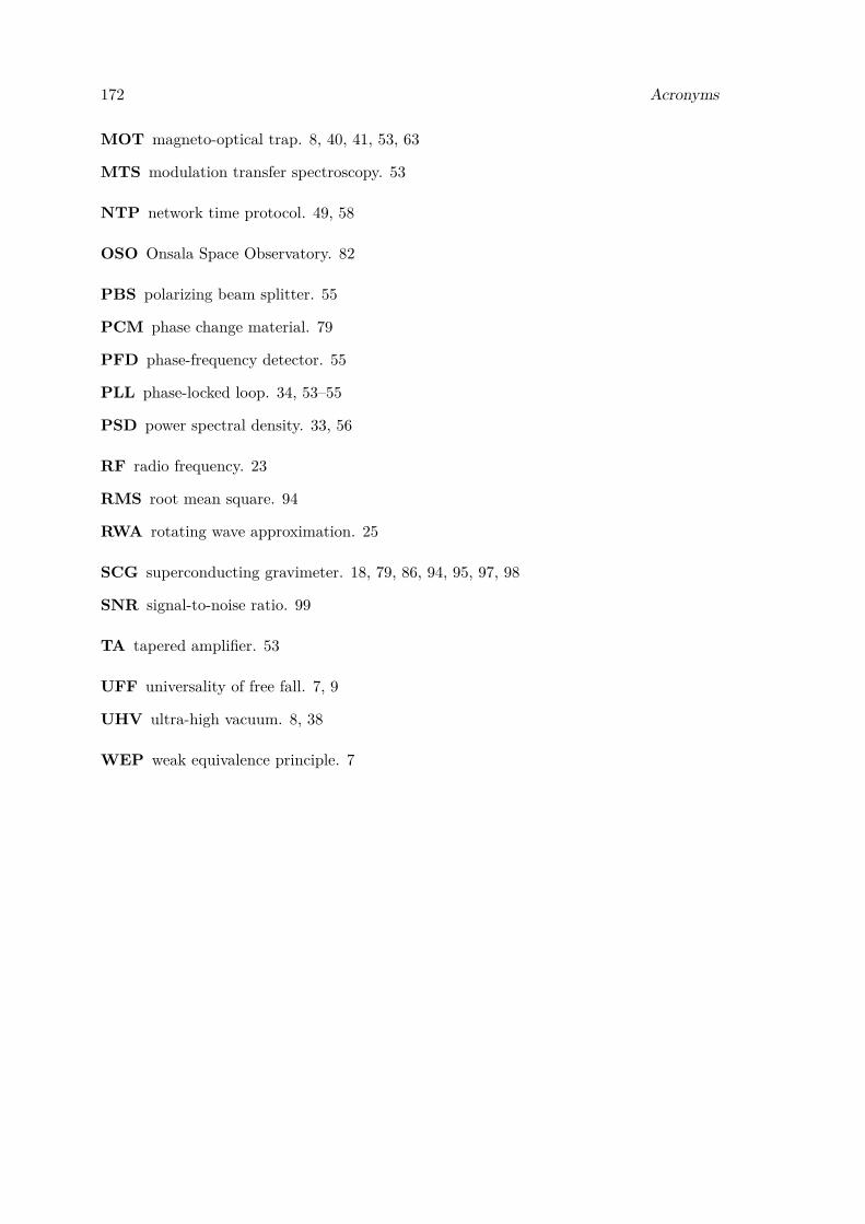
172 Acronyms
MOT magneto-optical trap. 8, 40, 41, 53, 63
MTS modulation transfer spectroscopy. 53
NTP network time protocol. 49, 58
OSO Onsala Space Observatory. 82
PBS polarizing beam splitter. 55
PCM phase change material. 79
PFD phase-frequency detector. 55
PLL phase-locked loop. 34, 53–55
PSD power spectral density. 33, 56
RF radio frequency. 23
RMS root mean square. 94
RWA rotating wave approximation. 25
SCG superconducting gravimeter. 18, 79, 86, 94, 95, 97, 98
SNR signal-to-noise ratio. 99
TA tapered amplifier. 53
UFF universality of free fall. 7, 9
UHV ultra-high vacuum. 8, 38
WEP weak equivalence principle. 7

Publications
Print• Mobile Quantum Gravity Sensor with Unprecedented Stability
C Freier, M Hauth, V Schkolnik, B Leykauf, M Schilling, H Wziontek, H-G Sch-erneck, J Müller, and A Peters. (June 2016) Journal of Physics: Conference Series723 12050
• The Effect of Wavefront Aberrations in Atom InterferometryV Schkolnik, B Leykauf, M Hauth, C Freier, and A Peters. Applied Physics B 120,311–316 (2015).
• Atom Interferometry for Absolute Measurements of Local GravityM Hauth, C Freier, V Schkolnik, A Peters, H Wziontek, and M Schilling. Pro-ceedings of the International School of Physics ‘Enrico Fermi’, Course 188, 557–586(2014).
• First Gravity Measurements using the Mobile Atom Interferometer GAINM Hauth, C Freier, V Schkolnik, A Senger, M Schmidt, and A Peters. AppliedPhysics B 113, 49–55 (2013).
• A Mobile High-Precision Absolute Gravimeter based on Atom Interfer-ometryM Schmidt, A Senger, M Hauth, C Freier, V Schkolnik, and A Peters. Gyroscopyand Navigation 2, 170–177 (2011).
Oral PresentationsOnly those presentations are listed where the thesis author is first author and presenter.
• Colloquium Talk, Séminaire Temps/Fréquence du SYRTE, Paris, France (2016)
• Invited Talk, École de Physique des Houches ”Advanced atomic sources and extremecooling of atoms and molecules: techniques and applications”, Les Houches, France(2016)
• Colloquium Talk, Nanyang Technical University, Singapore (2015)
• Colloquium Talk, National University of Singapore, Singapore (2015)
173

174 Acronyms
• Contributed Talk, Deutsche Physikalische Gesellschaft (DPG) Annual Meeting, Hei-delberg, Germany (2015)
• Colloquium Talk, Chalmers University, Gothenburg, Sweden (2015)
• Contributed Talk, ”Geodätische Woche” during the Intergeo Conference, Berlin, Ger-many (2014)
• Contributed Talk, Deutsche Physikalische Gesellschaft (DPG) Annual Meeting, Berlin,Germany (2014)
• Contributed Talk, International Association of Geodesy (IAG) Scientific Assembly,Potsdam, Germany (2013)
• Contributed Talk, Deutsche Physikalische Gesellschaft (DPG) Annual Meeting, Stuttgart,Germany (2012)
Poster PresentationsOnly those presentations are listed where the thesis author is first author and presenter.
• International Conference on Laser Spectroscopy (ICOLS), Singapore (2015)
• Deutsche Physikalische Gesellschaft (DPG) Annual Meeting, Hannover, Germany(2013)
• Young Atom Opticians Conference (YAO), Hannover, Germany, (2011)
• Deutsche Physikalische Gesellschaft (DPG) Annual Meeting, Dresden, Germany(2011)
Student SupervisionMaster Student
• Bastian LeykaufGradiometric Measurements with a Juggling Atomic Fountain(working title, in preparation)
Bachelor Students• Linos Hecht
Implementation of Components for Raman Sideband Cooling (2015)
• Marek MandelImplementierung des Versuchs ”Magneto-optische Falle” für das Fortgeschrittenen-praktikum (2014)
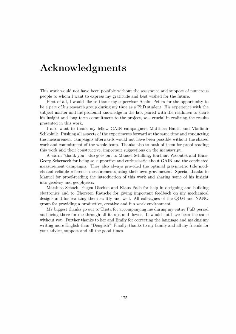
Acknowledgments
This work would not have been possible without the assistance and support of numerouspeople to whom I want to express my gratitude and best wished for the future.
First of all, I would like to thank my supervisor Achim Peters for the opportunity tobe a part of his research group during my time as a PhD student. His experience with thesubject matter and his profound knowledge in the lab, paired with the readiness to sharehis insight and long term commitment to the project, was crucial in realizing the resultspresented in this work.
I also want to thank my fellow GAIN campaigners Matthias Hauth and VladimirSchkolnik. Pushing all aspects of the experiments forward at the same time and conductingthe measurement campaigns afterwards would not have been possible without the sharedwork and commitment of the whole team. Thanks also to both of them for proof-readingthis work and their constructive, important suggestions on the manuscript.
A warm ”thank you” also goes out to Manuel Schilling, Hartmut Wziontek and Hans-Georg Scherneck for being so supportive and enthusiastic about GAIN and the conductedmeasurement campaigns. They also always provided the optimal gravimetric tide mod-els and reliable reference measurements using their own gravimeters. Special thanks toManuel for proof-reading the introduction of this work and sharing some of his insightinto geodesy and geophysics.
Matthias Schoch, Eugen Dischke and Klaus Palis for help in designing and buildingelectronics and to Thorsten Rausche for giving important feedback on my mechanicaldesigns and for realizing them swiftly and well. All colleagues of the QOM and NANOgroup for providing a productive, creative and fun work environment.
My biggest thanks go out to Trista for accompanying me during my entire PhD periodand being there for me through all its ups and downs. It would not have been the samewithout you. Further thanks to her and Emily for correcting the language and making mywriting more English than ”Denglish”. Finally, thanks to my family and all my friends foryour advice, support and all the good times.
175

176 Acronyms
Selbstständigkeitserklärung
Hiermit erkläre ich, die vorliegende Arbeit selbstständig und nur unter Verwendung derangegebenen Quellen und Hilfsmittel angefertigt zu haben. Ich habe mich anderweitignicht um einen Doktorgrad beworben und besitze einen solchen auch nicht. Die dem Ver-fahren zugrundeliegende Promotionsordnung der Mathematisch-NaturwissenschaftlichenFakultät der Humboldt Universität zu Berlin habe ich zur Kenntnis genommen.
Berlin, den May 30, 2017 Christian Freier
177