
EssaysinAppliedMacroeconomic Theory - MADOC€¦ · EssaysinAppliedMacroeconomic Theory...
155
Essays in Applied Macroeconomic Theory Inauguraldissertation zur Erlangung des akademischen Grades eines Doktors der Wirtschaftswissenschaften der Universität Mannheim vorgelegt von Giuseppe Corbisiero im Frühjahrssemester 2015
Transcript of EssaysinAppliedMacroeconomic Theory - MADOC€¦ · EssaysinAppliedMacroeconomic Theory...

Essays in Applied MacroeconomicTheory
Inauguraldissertation
zur Erlangung des akademischen Grades
eines Doktors der Wirtschaftswissenschaften
der Universität Mannheim
vorgelegt von
Giuseppe Corbisiero
im Frühjahrssemester 2015

Abteilungssprecher: Prof. Dr. Eckhard JanebaReferent: Prof. Dr. Michèle TertiltKorreferent: Prof. Dr. Klaus Adam
Tag der mündlichen Prüfung: 21. Juli 2015

A mio padre, a mia madre e ad Antonio.
E alla mia terra, alle sue rigogliose colline,
alla sua calura estiva, ai suoi cieli tersi d’inverno.

Acknowledgments
First and foremost, I am deeply indebted to my supervisor Michèle Tertilt for her invaluable
guidance and support along the process of my PhD. Her innumerable and insightful feedback
has constantly represented a stimulus for improvement of my approach to research, and this
work would not have been possible without it. My dissertation also benefited immensely from
thoughtful discussions with Klaus Adam. In particular, his suggestions crucially helped me
to develop my job market paper - Chapter 2 of this thesis.
Particular thanks go to Salvatore Piccolo for his great work and support in the co-writing
of the fourth chapter, and to Thomas Tröger for insightful discussions concerning the third
chapter of this thesis. I am also very grateful to Benjamin Born, Antonio Ciccone, Emanuele
Tarantino, Cezar Santos, Georg Dürnecker, Matthias Kehrig, and all other members of the
Mannheim Center for Macroeconomics and Finance for their helpful comments and sugges-
tions. I gratefully acknowledge the financial support from the DFG and the ERC Starting
Grant 313719.
Furthermore, I am very grateful to my PhD fellows from the CDSE for an inspiring and
enjoyable working environment. In particular, the weekly meetings with Michèle Tertilt,
Florian Exler, Vera Molitor, Henning Roth, Xiaodi Wang, and Xue Zhang constituted a
stimulating environment throughout the whole research process.
I was fortunate to have great friends at the university in Francesco Paolo Conteduca,
Niccolò Lomys, Alessandra Donini, Agustìn Arias, Oceane Briand, Vittorio Larocca, Clau-
dio Baccianti, Elena Rancoita, Florian Sarnetzki, Stefan Weiergräber, Timo Hoffmann, and
Christoph Esslinger, who always helped and supported me.
Last but not least, I thank my family - my parents Vincenzo e Luigia and my brother
Antonio - for their support throughout these last five years I have been living abroad.

Contents
Page
List of Figures v
List of Tables vii
1 General Introduction 11.1 Ch. 2: Banks’ Home Bias and Credit Traps in a Monetary Union . . . . . . . 31.2 Ch. 3: Labor Market Frictions and Fertility . . . . . . . . . . . . . . . . . . . . 41.3 Ch. 4: Family Ties, Institutions, and Income Inequality . . . . . . . . . . . . . 4
2 Banks’ Home Bias and Credit Traps 72.1 Introduction . . . . . . . . . . . . . . . . . . . . . . . . . . . . . . . . . . . . . 92.2 Model Setup . . . . . . . . . . . . . . . . . . . . . . . . . . . . . . . . . . . . . 14
2.2.1 Firms’ Problem . . . . . . . . . . . . . . . . . . . . . . . . . . . . . . . 152.2.2 Banks’ Problem . . . . . . . . . . . . . . . . . . . . . . . . . . . . . . . 182.2.3 Governments . . . . . . . . . . . . . . . . . . . . . . . . . . . . . . . . . 212.2.4 Central Bank . . . . . . . . . . . . . . . . . . . . . . . . . . . . . . . . . 21
2.3 Benchmark Case: Non-home-biased Banks . . . . . . . . . . . . . . . . . . . . 222.3.1 Equilibrium on the Market for Funds for a Given Asset Liquidation Value 232.3.2 Equilibrium with Endogenous Asset Liquidation Value . . . . . . . . . . 29
2.4 Model with Banks’ Home Bias . . . . . . . . . . . . . . . . . . . . . . . . . . . 322.4.1 Equilibrium on the Market for Funds for a Given Asset Liquidation Value 322.4.2 Equilibrium with Endogenous Asset Liquidation Value . . . . . . . . . . 37
2.5 Model Predictions, ECB’s Policy, and Lending in the EMU . . . . . . . . . . . 412.6 Conclusion . . . . . . . . . . . . . . . . . . . . . . . . . . . . . . . . . . . . . . 462.7 Appendix A. Proofs . . . . . . . . . . . . . . . . . . . . . . . . . . . . . . . . . 47
2.7.1 Proof of Lemma 1 . . . . . . . . . . . . . . . . . . . . . . . . . . . . . . 472.7.2 Proof of Proposition 1 . . . . . . . . . . . . . . . . . . . . . . . . . . . . 492.7.3 Proof of Lemma 2 . . . . . . . . . . . . . . . . . . . . . . . . . . . . . . 502.7.4 Proof of Proposition 2 . . . . . . . . . . . . . . . . . . . . . . . . . . . . 51
i

ii Contents
2.7.5 Proof of Proposition 3 . . . . . . . . . . . . . . . . . . . . . . . . . . . . 522.8 Appendix B. Supplementary Figures . . . . . . . . . . . . . . . . . . . . . . . . 54
3 Labor Market Frictions and Fertility 573.1 Introduction . . . . . . . . . . . . . . . . . . . . . . . . . . . . . . . . . . . . . 593.2 Model Setup . . . . . . . . . . . . . . . . . . . . . . . . . . . . . . . . . . . . . 63
3.2.1 Agents’ Problem . . . . . . . . . . . . . . . . . . . . . . . . . . . . . . . 643.2.2 Job Market Environment . . . . . . . . . . . . . . . . . . . . . . . . . . 663.2.3 Technology . . . . . . . . . . . . . . . . . . . . . . . . . . . . . . . . . . 673.2.4 Definition of the Equilibrium . . . . . . . . . . . . . . . . . . . . . . . . 68
3.3 Results . . . . . . . . . . . . . . . . . . . . . . . . . . . . . . . . . . . . . . . . 703.3.1 Job Market Equilibrium: Characterization . . . . . . . . . . . . . . . . 703.3.2 Job Market Frictions and Fertility . . . . . . . . . . . . . . . . . . . . . 74
3.3.2.1 Signal Technology and Fertility: Discussion . . . . . . . . . . . 753.3.3 Labor Market Regulation . . . . . . . . . . . . . . . . . . . . . . . . . . 773.3.4 Time Cost of Children . . . . . . . . . . . . . . . . . . . . . . . . . . . 79
3.4 Model Predictions vs. Data . . . . . . . . . . . . . . . . . . . . . . . . . . . . . 813.5 Conclusion . . . . . . . . . . . . . . . . . . . . . . . . . . . . . . . . . . . . . . 863.6 Appendix A: Definition of the Refinement H . . . . . . . . . . . . . . . . . . . 883.7 Appendix B: Proofs . . . . . . . . . . . . . . . . . . . . . . . . . . . . . . . . . 89
3.7.1 Lemma 1 and Proof . . . . . . . . . . . . . . . . . . . . . . . . . . . . . 893.7.2 Proof of Proposition 1 . . . . . . . . . . . . . . . . . . . . . . . . . . . . 903.7.3 Proof of Lemma 2 . . . . . . . . . . . . . . . . . . . . . . . . . . . . . . 923.7.4 Proof of Proposition 2 . . . . . . . . . . . . . . . . . . . . . . . . . . . . 953.7.5 Proof of Proposition 3 . . . . . . . . . . . . . . . . . . . . . . . . . . . . 963.7.6 Proof of Proposition 4 . . . . . . . . . . . . . . . . . . . . . . . . . . . 97
3.8 Appendix C: Robustness and Extensions . . . . . . . . . . . . . . . . . . . . . 1003.8.1 Binding Constraint at the Education Stage . . . . . . . . . . . . . . . . 1003.8.2 Policy Intervention . . . . . . . . . . . . . . . . . . . . . . . . . . . . . . 1023.8.3 Brief Discussion of Further Robustness . . . . . . . . . . . . . . . . . . 104
3.9 Appendix D: Supplementary Figures . . . . . . . . . . . . . . . . . . . . . . . . 107
4 Family Ties, Institution, and Income Inequality 1114.1 Introduction . . . . . . . . . . . . . . . . . . . . . . . . . . . . . . . . . . . . . 1134.2 Model Setup . . . . . . . . . . . . . . . . . . . . . . . . . . . . . . . . . . . . . 117
4.2.1 Public Good Production, Agents, and Environment . . . . . . . . . . . 1174.2.2 Timing of the Agents’ Decisions . . . . . . . . . . . . . . . . . . . . . . 1184.2.3 Functional Forms . . . . . . . . . . . . . . . . . . . . . . . . . . . . . . 119
iii
4.2.4 Definition of the Equilibrium . . . . . . . . . . . . . . . . . . . . . . . . 1194.3 Results . . . . . . . . . . . . . . . . . . . . . . . . . . . . . . . . . . . . . . . . 120
4.3.1 Parental Altruism, Public Good Provision and Income Distribution . . 1214.4 Model Predictions vs. Data . . . . . . . . . . . . . . . . . . . . . . . . . . . . . 1244.5 Discussion and Concluding Remarks . . . . . . . . . . . . . . . . . . . . . . . . 1264.6 Appendix: Proofs . . . . . . . . . . . . . . . . . . . . . . . . . . . . . . . . . . 128
4.6.1 Proof of Lemma 1 . . . . . . . . . . . . . . . . . . . . . . . . . . . . . . 1284.6.2 Proof of Proposition 1 . . . . . . . . . . . . . . . . . . . . . . . . . . . . 1294.6.3 Proof of Proposition 2 . . . . . . . . . . . . . . . . . . . . . . . . . . . . 1304.6.4 Proof of Proposition 3 . . . . . . . . . . . . . . . . . . . . . . . . . . . . 131
5 Bibliography 133


List of Figures
Page
2.1 Aggregate credit to non-financial corporations in the eurozone . . . . . . . . . 10
2.2 Commercial bank’s balance sheet . . . . . . . . . . . . . . . . . . . . . . . . . 19
2.3 Timing of events . . . . . . . . . . . . . . . . . . . . . . . . . . . . . . . . . . 22
2.4 Interest rate and lending as function of the aggregate liquidity . . . . . . . . . 36
2.5 Lending rates vs. ECB policy rate . . . . . . . . . . . . . . . . . . . . . . . . 44
2.6 Banks’ domestic sovereign holdings . . . . . . . . . . . . . . . . . . . . . . . . 45
2.7 Aggregate credit to non-financial corporations by GDP . . . . . . . . . . . . . 54
2.8 Aggregate credit to non-financial corporations . . . . . . . . . . . . . . . . . . 54
2.9 Home share of sovereign debt held by banks (2011) . . . . . . . . . . . . . . . 55
3.1 Female employment vs. TFR (OECD-21, year 2010) . . . . . . . . . . . . . . 59
3.2 The least cost separating equilibrium . . . . . . . . . . . . . . . . . . . . . . . 71
3.3 Optimal transfer . . . . . . . . . . . . . . . . . . . . . . . . . . . . . . . . . . 73
3.4 Better signal technology and its effect on fertility . . . . . . . . . . . . . . . . 76
3.5 Optimal transfer and better signal technology . . . . . . . . . . . . . . . . . . 77
3.6 Summary of the model results . . . . . . . . . . . . . . . . . . . . . . . . . . . 82
3.7 Proxies of labor market frictions vs. TFR . . . . . . . . . . . . . . . . . . . . 85
3.8 Equilibrium with constrained agents . . . . . . . . . . . . . . . . . . . . . . . 101
v
vi LIST OF FIGURES
3.9 Equilibrium with redistributive policy . . . . . . . . . . . . . . . . . . . . . . 103
3.10 Job market indicators and fertility . . . . . . . . . . . . . . . . . . . . . . . . 107
3.11 Youth financial dependence and fertility . . . . . . . . . . . . . . . . . . . . . 107
3.12 Job mismatch vs. other job market indicators . . . . . . . . . . . . . . . . . . 108
3.13 Job mismatch vs. youth financial dependence . . . . . . . . . . . . . . . . . . 108
3.14 Expenditure on education vs. job market indicators . . . . . . . . . . . . . . 109
3.15 Expenditure on education vs. youth financial dependence . . . . . . . . . . . 109
3.16 Households expenditure on education and fertility . . . . . . . . . . . . . . . 109
4.1 Family Ties and Governance Indicators . . . . . . . . . . . . . . . . . . . . . 115
4.2 Family Ties and Gini at Disposable Income . . . . . . . . . . . . . . . . . . . 125

List of Tables
Page
3.1 Correlations between TFR, education, and job market indicators . . . . . . . 84
4.1 Worldwide Governance Indicators (WGI) . . . . . . . . . . . . . . . . . . . . . 114
vii


Chapter 1
General Introduction


3
This thesis comprises three self-contained chapters that deal with macro-finance, growth
and development topics. All essays use an applied theory approach to investigate the impact
of frictions on the macroeconomy through their effect on individual incentives. In Chapter 2, I
study how banks’ exposure to their home country sovereign default risk affects unconventional
monetary policy in a monetary union. Chapter 3 finds asymmetric information friction to
be a possible cause for low fertility across developed countries. Chapter 4 is joint work with
Salvatore Piccolo, in which we study how stronger family ties reduce the quality of institutions
and increase income inequality in a country.
As all the chapters of this dissertation are written as independent papers, each of them
contains its own introduction and appendices that provide supplementary materials such as
proofs and extensions as well as additional graphs. Hence, the essays can be read in any
order. References from all three chapters can be found in a bibliography at the end of this
dissertation. In the remainder of this section, I provide a more detailed summary of each
essay.
1.1 Ch. 2: Banks’ Home Bias and Credit Traps in a
Monetary Union
Since the beginning of the recent financial crisis, the ECB has adopted measures to pro-
vide eurozone banks with sufficient liquidity and avoid the risk of a credit crunch. Never-
theless, banks’ lending has hardly reacted. Lending remained low mainly in countries where
sovereigns have been perceived risky since the euro sovereign debt crisis, instead banks’ do-
mestic sovereign debt holdings have largely increased. This paper provides a theory which
aims at explaining this facts. The model studies the effectiveness of central bank liquidity in-
jections aimed at boosting corporate lending. I model a monetary union where the financial
system is in distress and countries differ in the risk of sovereign default. The high lever-
age of banks, their dependence on market confidence, and their direct exposure to domestic
sovereign bonds make banking very vulnerable to the risk of default of their sovereigns. The
theoretical framework incorporates this feature by assuming that sovereign default spills over
to the country’s banks. Moreover, the model captures the general equilibrium interplay be-
tween liquidity, financial frictions, firms’ collateral, and lending. I find that the link between
domestic banking and sovereign default risk crucially affects how commercial banks respond
to monetary policy. In particular, I show that by injecting liquidity the central bank might

4 CHAPTER 1. GENERAL INTRODUCTION
finance the risky sovereign rather than boosting lending. I also show that sovereign default
risk in one country generates negative spillover effects on lending in the rest of the monetary
union via the collateral channel, i.e. it can reduce the price of asset used as collateral and
hence firms’ debt capacity. Thus, the effectiveness of unconventional measures is limited even
in countries that are not directly subject to the risk of sovereign default. The model sheds
light on the effects of the unconventional measures recently adopted by the ECB to tackle
the financial crisis and its aftermath.
1.2 Ch. 3: Labor Market Frictions and Fertility
Fertility rates largely differ across countries. In developed countries, fertility shows a pos-
itive cross-country correlation with income and female labor force participation. This fact
seems to contradict the common hypothesis in the fertility literature that a higher opportunity
cost of parental time depresses fertility. To understand this puzzle, I analyze an overlapping
generations model where fertility is endogenous and parents discount future utility of their
children. A main feature of my analysis is the presence of an asymmetric information friction
encountered by labor market entrants. The job market is modeled in line with the signal-
ing game literature following Spence (1973). I find that a larger incidence of asymmetric
information increases job market entrants’ joblessness time and their financial dependence on
parents, playing a crucial role for low fertility. Better education and labor market institutions
reduce information asymmetry and consequently have a two-fold positive effect on fertility:
First, they make children more affordable to young adults, who can start working earlier and
hence earn higher incomes. Second, they reduce children’s financial dependence on parents
and thereby lower child-rearing costs. By contrast, labor market rigidities can exacerbate
information asymmetry and depress fertility. The model predictions are consistent with the
empirical evidence in Europe. Countries with higher incidence of labor market frictions and
youth financial dependence on parents display lower fertility rates.
1.3 Ch. 4: Family Ties, Institutions, and Income Inequality
In this chapter, we address the question whether the strength of family ties can negatively
affect the quality of institutions in a country. In our theoretical framework, parents discount
future utility of their children and can exert a costly lobbying effort to provide them with
private benefits. Private benefits are obtained by diverting resources from the production of

5
a public good. As agents are atomistic, no one feels that her lobbying effort can influence the
amount of public good produced. The consequence is that at the aggregate level each agent
generates a negative externality that results in the underprovision of the public good. We
find that a higher degree of parental altruism – a proxy for stronger family ties – is negatively
associated with the provision of the public good. We use the latter as a proxy for the quality of
institutions. Moreover, the model points at a positive relationship between parental altruism
and ncome inequality. Evidence from Europe supports these results: European countries
display a negative correlation between the strength of family ties and World Bank estimates
of the quality of institutions, as well as a positive correlation between the strength of family
ties and the Gini coefficient at disposable income.


Chapter 2
Banks’ Home Bias and Credit Traps
in a Monetary Union

9
2.1 Introduction
The recent financial crisis has led to a severe reduction in the availability of credit to firms,
which resulted in an economic downturn. To combat the crisis and foster credit creation,
all major central banks have adopted measures that go beyond their traditional interest rate
policy. New unconventional policy measures - e.g. direct lending to financial institutions,
provision of liquidity to key credit markets, purchases of long term securities - have been
adopted to overcome the financial market impairments, which were constraining the process
of credit creation in spite of the reduction in policy interest rates (see e.g. Fahr, Motto,
Rostagno, Smets, and Tristani 2011, and Mishkin 2011).
To what extent can unconventional measures boost corporate lending in the presence of
financial instability? This paper addresses this question in the context of a monetary union,
where national governments issue risky sovereign debt. Recent events in the European Eco-
nomic and Monetary Union (EMU) make such analysis particularly interesting. Since 2010-
11, spreads on ten-year sovereign bond yields between Germany and Greece, Ireland, Por-
tugal, Spain, and Italy have increased dramatically. As these bonds are all denominated in
euro, differences in expected yield mainly represent differences in perceived sovereign default
risk (see e.g. Lane 2012 for more details on the European sovereign debt crisis).
Since the beginning of the crisis in 2008, the European Central Bank (ECB) has adopted
measures to provide eurozone banks with sufficient liquidity and avoid the risk of a credit
crunch (see Section 5 for more details). Nevertheless, lending has poorly reacted, particularly
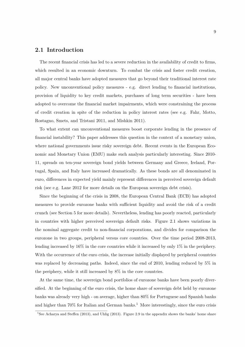
in countries with higher perceived sovereign default risks. Figure 2.1 shows variations in
the nominal aggregate credit to non-financial corporations, and divides for comparison the
eurozone in two groups, peripheral versus core countries. Over the time period 2008-2013,
lending increased by 16% in the core countries while it increased by only 1% in the periphery.
With the occurrence of the euro crisis, the increase initially displayed by peripheral countries
was replaced by decreasing paths. Indeed, since the end of 2010, lending reduced by 5% in
the periphery, while it still increased by 8% in the core countries.
At the same time, the sovereign bond portfolios of eurozone banks have been poorly diver-
sified. At the beginning of the euro crisis, the home share of sovereign debt held by eurozone
banks was already very high - on average, higher than 80% for Portuguese and Spanish banks
and higher than 70% for Italian and German banks.1 More interestingly, since the euro crisis1See Acharya and Steffen (2013), and Uhlig (2013). Figure 2.9 in the appendix shows the banks’ home share

10 CHAPTER 2. BANKS’ HOME BIAS AND CREDIT TRAPS
Figure 2.1: Aggregate credit to non-financial corporations in the eurozoneThe values of the series are normalized to 100 at January, 2008. Data source: BIS.
begun, domestic sovereign debt holdings of banks have increased the most exactly in those
countries where larger perceived risks of sovereign default emerged. From the last quarter of
2010 to the first quarter of 2013, the amount of banks’ sovereign holdings increased by 63%
in the peripheral eurozone countries while it increased by only 14% in the core countries (see
Figure 2.6 below for more details).
This paper provides a theory which aims at explaining this evidence. This theory relies
on the hypothesis that the high leverage of banks, their dependence on market confidence,
and their typical large exposure - even in “normal” times - to their sovereigns make banking
very likely to be affected by domestic sovereign default risk. In other words, the occurrence
of sovereign default is likely to produce a systemic shock in the country that would affect
domestic banks much more than foreign ones.2 The theoretical framework incorporates this
feature by assuming that banks are exogenously exposed to domestic sovereign default risk -
or “home biased.” The purpose is to analyze to what extent this feature can compromise the
effectiveness of the recent ECB’s unconventional monetary policy aimed at boosting lending,
and explain why we observe so different lending responses in the eurozone.
This model builds upon the literature hypothesizing that firms’ collateral eases finan-
cial frictions and increases debt capacity (see Hart and Moore 1994, 1998, Benmelech and
Bergman 2009, 2012, and the financial accelerator literature: Bernanke and Gertler 1989,
Kiyotaki and Moore 1997, Bernanke, Gertler, and Gilchrist 1999). In a stylized two-country
of sovereign exposure across eurozone countries in 2011.2This hypothesis is consistent with the methodology in use at credit rating agencies for determining riskassessments of financial institutions. Banks very rarely have a rating above their sovereign exactly for thereasons mentioned above: see e.g. “Sovereign Risk for Financial Institutions,” published Feb. 16, 2004,Standard & Poor’s.

11
monetary union, governments issue differently risky sovereign debt. In each country firms
need external funds to undertake projects generating returns in the following two periods.
Returns cannot be verified by banks - à la Hart and Moore (1989, 1998) - but firms can
access bank loans by pledging their asset as collateral. The price of the asset, which limits
firms’ debt capacity, is endogenously determined in a market whose structure follows Shleifer
and Vishny (1992). As in Benmelech and Bergman (2012), financial distress is captured by
a liquidity shock forcing a share of firms to liquidate their asset; unconventional measures
are modeled in reduced-form by assuming that the central bank directly injects liquidity into
commercial banks’ balance sheet.
In equilibrium, liquidity injections can reduce the interest rate, increase the value of the
collateral and firms’ debt capacity, and successfully contrast the lending reduction during
an economic downturn. In this framework, I ask whether the link between banking and
sovereign risk threatens the monetary transmission mechanism. In particular, I analyze how
it affects the interplay between liquidity, financial frictions, the price of firms’ collateral, and
corporate lending. For ease of exposition, the analysis is conducted comparing two scenarios.
I analyze first a benchmark case in which banks are not exposed to the risk of their sovereign.
The second scenario - which I refer to as “banks’ home bias” - introduces bank exposure to
domestic sovereign default risk. This is captured by assuming that the occurrence of sovereign
default exogenously produces the bankruptcy of domestic banks.3
In the benchmark case, an integrated market for firms’ collateral guarantees an equal prop-
agation of the monetary policy effects in both countries. Liquidity injections increase banks’
supply of funds and lower the equilibrium interest rate. The discounted price of the asset
increases, the borrowing constraint of firms relaxes, and hence lending increases. Moreover,
the higher lending endows firms with more funds, which will be used to bid more aggressively
for the assets liquidated by firms in financial distress. The liquidation price of the asset will
increase and banks, anticipating this dynamic, banks are willing to further increase lending.
Sovereign default risks have no impact on monetary transmission and lending responses are
equal across the union countries. Similarly as in Benmelech and Bergman (2012), a limita-
tion to monetary policy effectiveness emerges only if a too large share of firms are forced to
liquidate the asset - which proxies for the severity of the crisis. In this case, lending remains
constrained at a suboptimal level, despite further injections of liquidity from the central bank.
3The mechanisms of the paper are robust to a different and less restrictive formulation of this assumption.See Section 2.2 for a detailed discussion.

12 CHAPTER 2. BANKS’ HOME BIAS AND CREDIT TRAPS
In the “banks home bias” scenario, banks are exposed to the default risk of their sovereign.
If in the next period sovereign default occurs, domestic banks go bankrupt and do not enjoy
any return. This feature crucially affects their present investment decision. Compared to
an investor who is not exposed to this risk, they underestimate the expected return on
investments repaying in the future state of the world where sovereign default occurs.
Suppose that a country has risky sovereign debt, while in the other the sovereign always
repays. If the interest rate on firm loans equals the level at which the risky country’s sovereign
bonds are traded, banks’ home bias prevents the risky country’s lending rate from further
reductions. Consequently, despite further injections of liquidity from the central bank, credit
to firms remains constrained at low levels. Risky country’s banks use instead the additional
liquidity injected to underwrite domestic sovereign debt. The reason is that, although firm
loans always guarantee repayment up to the asset liquidation value, any positive return
in the future state of the world where domestic sovereign default occurs does not increase
home biased banks’ expected profit. Hence, these banks are not willing to acknowledge a
differential between the interest rates on firm loans and on risky domestic sovereign debt.
Despite liquidity injections, the lending rate remains constant, preventing the discounted
price of collateral and the amount of lending from increasing.
Further reductions in the lending rate can only realize if liquidity injections are so forceful
that the last unit of newly issued sovereign debt is bought by a domestic bank. Only beyond
this threshold, central bank’s liquidity injections have further effects on lending in the risky
country, reducing the interest rate on firm loans, and expanding the amount of lending. By
contrast, in the safe country of the monetary union an increase in the liquidity injected always
produces a reduction in the lending rate and hence an increases in the amount of lending.
Thus, with home biased banks, monetary policy can have asymmetric effects on lending across
the monetary union countries.
Section 4 argues that this mechanism sheds light on the effects of the unconventional mea-
sures recently adopted by the ECB to tackle the financial crisis and its aftermath. Concerning
a forceful use of expansionary monetary policy, although the mechanism described seems to
recommend the use of forceful unconventional measures, a more subtle implication must
be considered. To be effective in the risky countries, the unconventional measures need to
be sufficiently forceful to substantially increase domestic banks’ exposure to sovereign debt.
However, this may strengthen the non-desirable link between sovereign risk and domestic

13
banking - which originates the above-described impairment of the monetary transmission
mechanism.
In the model, the exposure of one country’s banks to domestic sovereign risk can generate
a second important effect - namely, a negative spillover on lending in the other union country,
which will persist regardless of the central bank intervention. Country A’s banks rationally
anticipate that, if tomorrow country B’s government declares insolvency, its banks will go
bankrupt. Firms with deposits in those banks will have less funds to buy liquidated asset. As
result, the expected price of collateral can lower in the whole monetary union. In this case,
firms’ debt capacity and lending will be negatively affected in country A too, despite the
best efforts of the central bank. The extent to which unconventional measures can stimulate
lending will be limited, even in those economies which are not characterized by high sovereign
default risk.4
Benmelech and Bergman (2012) is the paper most closely related to mine. They study
unconventional monetary policy in a model with financial frictions between borrowers and
lenders as in Hart and Moore (1989, 1994, 1998), and a structure of the market for liqui-
dated assets as Shleifer and Vishny (1992). They find that, despite the best efforts of the
central bank to stimulate lending, banks may rationally choose to hoard liquidity during
monetary expansions rather than lending it out. My model focuses on features characterizing
the eurozone: a unique central bank, independent national governments issuing sovereign
debt, asymmetric sovereign default risks, and - crucially - banks’ home bias. So augmented,
the model highlights further limits on monetary policy effectiveness than those already ana-
lyzed by Benmelech and Bergman (2012), shedding light on the effects of the unconventional
measures recently adopted by the ECB to tackle the crisis.
Eurozone banks’ exposure to domestic sovereign debt has recently captured the attention of
the literature. Battistini, Pagano, and Simonelli (2014) address empirically the relationship
between the divergence in EMU countries’ sovereign yields and the simultaneous increase
in the home share of banks’ sovereign debt portfolios. They find that banks in peripheral
countries increase their domestic exposure as country risk increases. Acharya and Steffen
(2013) provide an empirical investigation of the “carry trade” by banks, which fund themselves
in the wholesale market and invest in risky sovereign bonds. They show that banks’ domestic
exposure increases over time partly because of the ECB funding these positions. Broner,4Section 5 discusses a methodology - based on Benmelech and Bergman (2011) - to test empirically thisspillover mechanism. The analysis, however, is left for future research.

14 CHAPTER 2. BANKS’ HOME BIAS AND CREDIT TRAPS
Erce, Martin, and Ventura (2014) address the euro sovereign debt crisis with a model relying
on creditor discrimination and crowding-out effects, showing that domestic debt purchases
reduce growth and welfare, possibly leading to self-fulfilling crises. In Uhlig (2013), banks’
exposure to domestic sovereign debt results from the incentive of risky countries’ regulators
to allow their banks to hold home risky bonds, getting to borrow more cheaply, and effectively
shifting the risk of some of the potential sovereign default losses on the common central bank.
Livshits and Schoors (2009) also argue that the banking crises, triggered by defaults, are due
to inadequate prudential regulations, and provide supporting evidence from the Russian 1998
crisis. In general, this literature supports the hypotheses that eurozone banks are exposed
to domestic sovereign default risk, and that sovereigns guarantee higher returns to home
investors. The focus of these papers is on the reasons that may have generated the large
exposure of eurozone banks to sovereign debt. By contrast, my analysis concentrates on the
consequences of the link between sovereign risk and domestic banking for the effectiveness of
monetary policy aimed at stimulating lending during a crisis.
The rest of the paper is organized as follows. Section 2 presents the model setup. Section
3 analyzes the benchmark case where banks are not home biased. Section 4, which contains
the main analysis, studies the effect of banks’ home bias on the monetary transmission mech-
anism. Section 5 discusses the model predictions in the light of the policy implemented by
the ECB and the lending response during the euro crisis. Section 6 concludes.
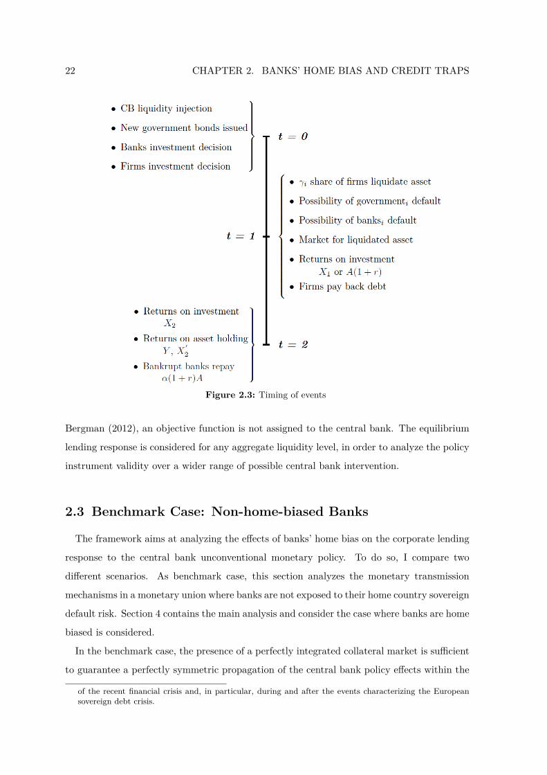
2.2 Model Setup
The setup is a stylized 3-period general equilibrium framework, constituted by two economies
in a monetary union. There is a unique central bank, and each of the two economies is com-
posed of a continuum of firms, a set of commercial banks which can supply funds to firms,
a government issuing sovereign bonds in fixed supply, with exogenous risks of default on
sovereign debt, possibly different across countries. Characterizing features of the model are:
(i) financial friction between borrowers and lenders à la Hart and Moore (1998), which is
caused by the non verifiability of firms project returns, and implies that firms need to pledge
their asset as collateral to access bank loans; (ii) endogenous market for firms collateral à la
Shleifer and Vishny (1992); (iii) possibility of central bank liquidity injections into banks, à
la Bemelech and Bergman (2012); (iv) banks’ exposure to domestic sovereign default risk. In
the following, the model setup is described in details. For convenience, Figure 2.3 compre-
15
hensively summarizes the timing of events.
2.2.1 Firms’ Problem
Each of the two countries, R and S, is populated by a continuum of firms Bi, whose measure
is normalized to unity. Each firm is endowed with an identical preexisting asset and different
initial wealth levels A. These levels are i.i.d. draws according to probability measure PA
over [0, I], with associated cumulative distribution function F (A). Each firm has an identical
opportunity to undertake a new project, which requires an initial monetary investment of I
at t = 0, and generates returns X1 at t = 1 and X2 at t = 2, with I < X1 < X2. Firms
can borrow from domestic or foreign commercial banks in order to undertake the project.
It is convenient to define each firm’s borrowing requirement as the difference between the
cost of the project and the firm’s initial wealth, B ≡ I − A. Let F (B) be the cumulative
distribution function according to which firms’ borrowing requirements B are distributed over
the interval [0, I]. Firms can invest in the project - if they obtain sufficient funds from banks
- or deposit their initial wealth in domestic banks,5 earning a return that will be determined
by the equilibrium interest rate.
As in Benmelech and Bergman (2012), firms face an idiosyncratic liquidity shock: at t = 1,
a fraction γi of country i’s firms are forced to liquidate their asset and to consume all their
available wealth.6 A higher γi proxies for a higher aggregate liquidity shock hitting the
economy. Therefore, the level of γi captures the financial crisis magnitude.7 The price of
liquidated asset P is endogenously determined. There is a unique market for liquidated asset
across the two countries. Suppliers of the asset are those firms hit by the liquidity shock,
operators are all the other firms in the union. Buying an additional asset generates a return
Y > 0 at t = 2. This assumption implies that firms spared by the liquidity shock are willing
to buy liquidated assets. Similarly, holding the asset generates a return X′2 > Y at t = 2,
which implies that firms spared by the liquidity shock do not voluntarily liquidate their asset
at t = 1.8 I use a further technical assumption, that the return guaranteed by the additional
asset does not exceed the investment required to undertake the project, Y < I.9
5I assume that firms cannot deposit their wealth with foreign banks. In this setup it would be equivalent toassuming that depositing funds with foreign banks has a sufficiently high constant marginal cost.
6Ex-ante, the identity of the firms experiencing the liquidity shock at t = 1 is unknown.7I allow for different cross-country level of γ, showing that the main results do not rely on the cross-countrydifference or equality in the values of γ.
8See Benmelech and Bergman (2012), p. 3008.9This assumption implies that the time-0 expected price of liquidated asset, bounded from above by Y , isalways smaller than than the investment needed to undertake the project, then the financial friction is

16 CHAPTER 2. BANKS’ HOME BIAS AND CREDIT TRAPS
To summarize, at t = 0 a country i’s firm, whose initial wealth is A and who faces an
interest rate on loans rf 10 and an interest rate on deposits rdi , maximizes its expected payoff
by choosing between undertaking the project, which may imply borrowing an amount b ∈ R+
from banks, and depositing its initial wealth in the domestic bank.11 However, the presence of
financial friction requires that the financial contract is incentive compatible, which can limit
the firm’s ability to obtain from banks and hence to undertake the project. Define Ξ (b, ·)
a financial contract including b as one of its elements,12 and Ξ the set of feasible financial
contracts. The financial friction constrains the amount of obtainable funds b to be an element
of a feasible financial contract, b : Ξ (b, ·) ∈ Ξ.
Therefore, undertaking the project guarantees a time-0 expected payoff of:
V1 = γi[1IX1 + P −
(1 + rf
)b]
+ (1− γi)[1IX2 + x
(1IX1 −
(1 + rf
)b)
+ (1− x)(1IX1 −
(1 + rf
)b) YP
+X′2
], (2.1)
where 1I is an indicator function assuming value 1 if debt and the non-deposited initial wealth
are sufficient to invest in the project, b + (A− a) ≥ I, and 0 otherwise. With probability
γi, at t = 1 the firm is hit by the liquidity shock and is forced to liquidate the asset and to
consume its wealth, constituted by the project first return X1 and the liquidation value of
the asset P , after repaying the loan to the bank,(1 + rf
)b. With probability 1− γi the firm
is not hit by the liquidity shock and can continue its business until time-2, when the project
generates X2 and the asset generates X ′2. At time-1, the firm can use the share 1 − x, with
x ∈ [0, 1], of its wealth X1−(1 + rf
)b to buy additional assets at a price P and guaranteeing
return Y at time-2.
Alternatively, depositing the initial wealth A in the domestic bank at interest rate rdi leads
to an expected payoff equal to
V2 = γi[(
1 + rdi
)A+ P
]never negligible. See Section 3.
10Here rf represent both the cases of a loan from a domestic bank, whose interest rate is rfDi , and the one of
a loan from a foreign bank, whose interest rate is rfFj
11The lower index of an interest rate, i, j, indicates the country of residence of the bank, while the upperindex indicates whether funds are deposited, d, or they are lent to domestic firms, fD, foreign firms, fF ,domestic government, gD, or foreign government, gF .
12A financial contract is a three-dimensional vector that specifies: (i) the amount of funds lent at t = 0, (ii)the time-1 repayment, and (iii) the penalty in case of no repayment. See Section 3.1.1, which characterizethe optimal financial contract.

17
+ (1− γi)[y(1 + rdi
)A+ (1− y)
(1 + rdi
)AY
P+X
′2
]. (2.2)
Also in this case, the liquidity shock forces the firm to consume its time-1 wealth with prob-
ability γi. The firm’s wealth is constituted by the gross return on time-0 deposit(1 + rdi
)A
and the liquidation value of the asset P . With probability 1 − γi the firm is not hit by the
liquidity shock and can continue its business until time-2. At t = 2, the asset generates re-
turn X ′2, and the additional assets bought in the previous period, using 1−y share of wealth,
guarantee a gross return equal to(1 + rdi
)YP (1− y)A.13
Therefore, in the scenario where banks are not home biased, the profit maximization prob-
lem of a firm whose initial wealth is A can be written as follows:
maxξ∈{0,1}, b, x∈[0,1], y∈[0,1]
ξV1 + (1− ξ)V2 ,
s.t.
b: Ξ(b,·)∈Ξ, if ξ=1
b=0, otherwise
(2.3)
Banks’ exposure to domestic sovereign default risk does not modify the representation of
the firm’s expected payoff from undertaking the project, hence V1B = V1. However, the
return on deposits is affected by the risk of bank bankruptcy. Hence, in the banks’ home bias
scenario the firm’s expected payoff of depositing the initial wealth in the bank is modified in
the following way:
V2B = γi[(1− ρi)
(1 + rdi
)A+ ρiα
(1 + rdi
)A+ P
]
+ (1− γi){
(1− ρi)[y(1 + rdi
)+ (1− y)
(1 + rdi
) YP
]A+ ρiα
(1 + rdi
)A+X
′2
}. (2.4)
Differently than in the previous case, with probability ρi country i’s banks go bankrupt at
t = 1, hence they only repay α(1 + rdi
)A at t = 2, with α ∈ (0, 1], rather than
(1 + rdi
)A
at t = 1.14 Given the different expected payoff from depositing funds in the bank, V3, in the
banks’ home bias scenario the profit maximization problem of a firm whose initial wealth is
A is represented by:
13Without loss of generality - given that the equilibrium interest rate on deposit always equals the equilibriuminterest rate on loans - firms are not allowed to borrow funds simply to deposit them in the bank.
14See the banks’ problem below for more details about the manner in which banks’ exposure to domesticsovereign default risk is modeled.

18 CHAPTER 2. BANKS’ HOME BIAS AND CREDIT TRAPS
maxξ∈{0,1}, b, x∈[0,1], y∈[0,1]
ξV1B + (1− ξ)V2B , (2.5)
subject to the same constraint in the maximization problem (2.3), which can be interpreted
similarly.
2.2.2 Banks’ Problem
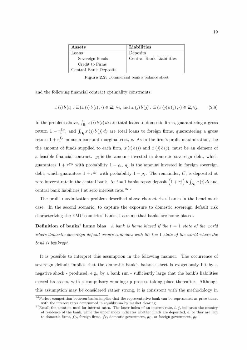
Each of the two economies includes a large number n of competitive commercial banks, all
identical, whose balance sheet is illustrated in Figure 2.2.
The total amount of funds that a country i’s bank can invest at time-0 is given by the sum
of deposits that the bank collects from firms not investing in the project and l - the single
bank’s share of the aggregate central bank liquidity injection L - with l = Ln . Define Ai the
subset of Bi constituted by those domestic firms ı who want to deposit a positive amount of
funds in that bank, Ai : {ı ∈ Bi : a (ı) > 0}. Then the maximum amount of firms deposits
that the bank can collect equals´Aia (ı) dı. The bank can decide how much to accept of it,
h´Aia (ı) dı, with h ∈ [0, 1]. Then it can share h
´Aia (ı) dı+l among the different investment
opportunities: loans to domestic or foreign firms, underwriting domestic or foreign sovereign
debt, holding as reserves in the central banks funds not lent out.15 Lending to foreign firms
has an operating constant marginal cost, c > 0.
Define Bi (Bj) the subset of Bi (Bj) constituted by those domestic firms ı (foreign firms )
who apply for loans to that bank, Bi : {ı ∈ Bi : b (ı) > 0}, Bj :{ ∈ Bj : b () > 0
}. For each
of these loans applications, b (ı) and b (), the bank decides how much of the required funds
to grant, x (ı) , x () ∈ [0, 1], and then how much domestic and sovereign debt to underwrite.
Therefore a bank maximizes its total time-1 expected payoff, given by:
(1 + rfDi
) ˆBi
x (ı) b (ı) dı+(1 + rfFi − c
) ˆBj
x () b () d
+ (1− ρi) (1 + rgD) gi + (1− ρj) (1 + rgF ) gj + C −(1 + rdi
)h
ˆAi
a (ı) dı− l , (2.6)
over the decision variables x (ı) ∈ [0, 1] , x () ∈ [0, 1] , gi, gj , h ∈ [0, 1], subject to the following
resources constraint:
ˆBi
x (ı) b (ı) dı+ˆ
Bj
x () b () d+ gi + gj ≤ hˆ
Ai
a (ı) dı+ l , (2.7)
15For simplicity, assume that both the interest rates on central bank deposits and liabilities equal zero.
19
Assets LiabilitiesLoans Deposits
Sovereign Bonds Central Bank LiabilitiesCredit to Firms
Central Bank DepositsFigure 2.2: Commercial bank’s balance sheet
and the following financial contract optimality constraints:
x (ı) b (ı) : Ξ (x (ı) b (ı) , ·) ∈ Ξ, ∀ı, and x () b () : Ξ (x () b () , ·) ∈ Ξ,∀. (2.8)
In the problem above,´Bix (ı) b (ı) dı are total loans to domestic firms, guaranteeing a gross
return 1 + rfDi , and´Bjx () b () d are total loans to foreign firms, guaranteeing a gross
return 1 + rfFi minus a constant marginal cost, c. As in the firm’s profit maximization, the
the amount of funds supplied to each firm, x (ı) b (ı) and x () b (), must be an element of
a feasible financial contract. gi is the amount invested in domestic sovereign debt, which
guarantees 1 + rgD with probability 1 − ρi, gj is the amount invested in foreign sovereign
debt, which guarantees 1 + rgF with probability 1 − ρj . The remainder, C, is deposited at
zero interest rate in the central bank. At t = 1 banks repay deposit(1 + rdi
)h´Aia (ı) dı and
central bank liabilities l at zero interest rate.1617
The profit maximization problem described above characterizes banks in the benchmark
case. In the second scenario, to capture the exposure to domestic sovereign default risk
characterizing the EMU countries’ banks, I assume that banks are home biased.
Definition of banks’ home bias A bank is home biased if the t = 1 state of the world
where domestic sovereign default occurs coincides with the t = 1 state of the world where the
bank is bankrupt.
It is possible to interpret this assumption in the following manner. The occurrence of
sovereign default implies that the domestic bank’s balance sheet is exogenously hit by a
negative shock - produced, e.g., by a bank run - sufficiently large that the bank’s liabilities
exceed its assets, with a compulsory winding-up process taking place thereafter. Although
this assumption may be considered rather strong, it is consistent with the methodology in16Perfect competition between banks implies that the representative bank can be represented as price taker,
with the interest rates determined in equilibrium by market clearing.17Recall the notation used for interest rates. The lower index of an interest rate, i, j, indicates the country
of residence of the bank, while the upper index indicates whether funds are deposited, d, or they are lentto domestic firms, fD, foreign firms, fF , domestic government, gD, or foreign government, gF .

20 CHAPTER 2. BANKS’ HOME BIAS AND CREDIT TRAPS
use at credit rating agencies for determining financial institutions risk assessments.18The as-
sumption can be relaxed, assuming instead that the occurrence of sovereign default implies
domestic banks’ bankruptcy only with some probability q, with 0 < q < 1. This alternative
formulation offers a simple way to interpret the possibility that only a share of banks would
go bankrupt after the sovereign default, with the technical advantage of still using a repre-
sentative commercial bank for each country. Proofs can be easily adapted to show that all
the model results are robust to this alternative formulation.19
In the banks’ home biased scenario, the time-1 expected payoff of a country i’s bank is
given by:
(1− ρi)[(
1 + rfDi
) ˆBi
x (ı) b (ı) dı+(1 + rfFi − c
)ˆBj
x () b () d
+ (1 + rgD) gi + (1− ρj) (1 + rgF ) gj + C −(1 + rdi
)h
ˆAi
a (ı) dı− l], (2.9)
which the bank maximizes over the decision variables x (ı) ∈ [0, 1] , x () ∈ [0, 1] , gi, gj , h ∈
[0, 1], and subject to the resources and financial contract optimality constraints (2.7) and (2.8)
above. Terms have a similar interpretation as those in problem (2.6). The only difference
consists in the fact that, with probability ρi, sovereign default occurs at t = 1 implying
domestic banks bankruptcy. A bankrupt bank does not enjoy any profit, and bankruptcy
implies that there is no continuation value. Therefore, any positive return in the time-1 state
of the world where the bank is bankrupt does not increase the bank’s time-0 expected profit,
which remains constant at 0.20
To capture a negative liquidity shock that sovereign default can impose on the domestic
demand for liquidated assets, I assume that a firm who deposited its initial wealth in a
bankrupt bank, at t = 1 has not immediate access to the recoverable funds, that cannot be
used to purchase liquidated assets. At t = 2 the firm will recover a fraction α ∈ (0, 1] of the
18See, e.g., “Sovereign Risk for Financial Institutions,” published Feb. 16, 2004, Standard & Poor’s. Banksrarely have a rating above their sovereign, as “banking is more likely than any other industry to be directlyor indirectly affected by any sovereign default or other such crisis. This vulnerability is due to the extremelyhigh leverage of banks (compared to corporates), the volatile valuation of their assets and liabilities in acrisis, their dependence on [market] confidence (which can disappear in a crisis), and their typically largedirect exposure to their sovereigns. Bank ratings, therefore, with few exceptions, logically should notexceed those of their sovereigns.” This argument should even more strongly apply to eurozone banks, giventhe above presented evidence about their sovereign bond portfolios with large home country shares.
19See, e.g., the proof of Proposition 2.20The bank’s maximization problem (5) assumes that the country j’s sovereign default probability is invariant
in the occurrence of country i’s sovereign default. For more details on this assumption, see Section 2.3.
21
gross return it would have got in the case of no bank’s bankrupt, namely α(1 + rdi )A. 21
2.2.3 Governments
In each country i, there is a government issuing risky sovereign debt in fixed supply, Gi ≥ 0.
If in country i sovereign default occurs, country i’s government does not repay to bondholders.
An objective function is not assigned to governments, so sovereign default is not strategic. For
each country there is an exogenous risk that the government is forced to declare insolvency,
which equals ρi, with ρR > 0 and ρR ≥ ρS ≥ 0. For simplicity, I assume that the sovereign
default risks of the two countries governments are not correlated. As the main cross-country
comparison below consists in a risky country’s equilibrium lending response measured against
a safe country’s one, this assumption is not much restrictive. Nevertheless, it can be easily
verified that the model mechanisms would still stay in place, reduced in magnitude only, for
positive correlation smaller than one, and would be amplified for negative correlation.
Outside the monetary union there are international investors willing to buy sovereign bonds
at an interest rate compensating for their risk, rgoviint = ρi1−ρi .
22
2.2.4 Central Bank
As in Benmelech and Bergman (2012), the central bank directly injects funds into com-
mercial banks by moving the central bank liabilities entry of the banks’ balance sheet. As
banks are assumed to be identical, apart from the difference in the sovereign debt exposure
across countries, I assume that the central bank cannot differently inject funds across banks.
Therefore, for an aggregate liquidity injection equal to 2L, L is the liquidity injection in each
union country’s bank system, and l the liquidity injected in each single bank, with l = Ln ,
where n is the number of commercial banks resident in each country.
The direct liquidity injection into commercial banks is meant to capture unconventional
monetary policy, which has been largely used by all the major central banks, the ECB in-
cluded, since the occurrence of the recent financial crisis.23 Similarly to Benmelech and21It is possible to interpret this assumption as follows. In case of bankruptcy, any asset of the bank is liquidated
in a compulsory winding-up process, with all creditors being guaranteed equal treatment. However, thetiming of the procedure implies that creditors do not have immediate access to liquid funds, obtaining therecoverable funds only in the following period.
22At rgoviint = ρi
1−ρiinvesting in sovereign bonds guarantees the same expected return of a risk free investment
with zero interest rate. Assuming rgoviint = ρi
1−ρidoes not reduce the generality of the results, as a level
rgoviint > ρi
1−ρiwould simply shift upwards the equilibrium interest rate for liquidity levels exceeding a
certain threshold, without producing any substantial change in the comparison between the banks’ homebias scenario and the benchmark case.
23Section 4 below considers in more details the policy measures undertaken by the ECB since the occurrence
22 CHAPTER 2. BANKS’ HOME BIAS AND CREDIT TRAPS
Figure 2.3: Timing of events
Bergman (2012), an objective function is not assigned to the central bank. The equilibrium
lending response is considered for any aggregate liquidity level, in order to analyze the policy
instrument validity over a wider range of possible central bank intervention.
2.3 Benchmark Case: Non-home-biased Banks
The framework aims at analyzing the effects of banks’ home bias on the corporate lending
response to the central bank unconventional monetary policy. To do so, I compare two
different scenarios. As benchmark case, this section analyzes the monetary transmission
mechanisms in a monetary union where banks are not exposed to their home country sovereign
default risk. Section 4 contains the main analysis and consider the case where banks are home
biased is considered.
In the benchmark case, the presence of a perfectly integrated collateral market is sufficient
to guarantee a perfectly symmetric propagation of the central bank policy effects within the
of the recent financial crisis and, in particular, during and after the events characterizing the Europeansovereign debt crisis.

23
union. Proposition 1 shows that the lending response to the central bank liquidity injections
is equal across the union countries, independently of cross-country differences in sovereign
default risk and in the share of firms hit by the liquidity shock and forced to liquidate
the asset. Furthermore, positive sovereign default risks do not imposes further restrictions
on monetary policy effectiveness to those already highlighted by Benmelech and Bergman
(2012) and produced by the gravity of the financial crisis, in other words by the magnitude
of the liquidity shock forcing firms to liquidate their asset.
In the following, I characterize first the implications of the financial friction on the market
for funds equilibrium when the asset liquidation value is given. Then the analysis includes
the market for liquidated asset and considers the interplay between liquidity injected by the
central bank, time-0 investment decisions and the equilibrium price of collateral.
2.3.1 Equilibrium on the Market for Funds for a Given Asset Liquidation
Value
The demand for funds comes from those firms who undertake the project and from govern-
ments which supply sovereign debt. Banks supply funds that they obtain from firms deposits
and central bank liquidity injections. Given an asset liquidation value P , market clearing
implies that the equilibrium interest rates adjust such that the total effective demand for
funds equals the total effective supply. The presence of financial friction - here modeled as
unverifiability of the firm project returns, following Hart and Moore (1989, 1998) - crucially
affects firms’ effective demand for funds and banks’ supply of loans, as discussed in details
in the following paragraph.
Firms’ demand for funds To undertake the project at t = 0, a firm with initial wealth
A needs to borrow an amount b ≥ I − A from commercial banks. The project returns X1
and X2 are unverifiable, i.e. bank’s claim on these returns cannot be exerted. Each firm,
however, is also endowed with a preexisting asset that can be liquidated at t = 1 and pledged
as collateral to access the bank’s loan. A crucial feature of the optimal financial contract
is the investor’s right to foreclose on the firm’s asset in case of no repayment. Given the
returns scheme assumed, the threat of liquidation exerted by the creditor bank induces the
firm to repay at t = 1. Following Benmelech and Bergman (2012), I assume that at t = 1
the firm has all the bargaining power in renegotiating its debt obligation with its bank. This
implies that a firm is never able to commit to repay at t = 1 an amount exceeding the asset

24 CHAPTER 2. BANKS’ HOME BIAS AND CREDIT TRAPS
liquidation value P .24 In the described framework, a financial contract between a firm and a
bank is constituted by three elements: (i) the time-0 amount of funds borrowed by the firm,
b; (ii) the time-1 repayment from the firm to the bank, b(1 + rf
); (iii) the penalty that the
bank can enforce in case of no repayment, namely forcing the firm to liquidate the project at
t = 1. A financial contract underwritten at time-0 is optimal if and only if it specifies a value
of the loan b such that b(1 + rf
)≤ P , as any time-1 repayment exceeding this threshold will
not take place in equilibrium.25
The characterization of the optimal financial contract allows to simplify the financial con-
tract feasibility constraint, represented in the firm’s profit maximization (2.3) as b : Ξ (b, ·) ∈
Ξ, in the following manner: b(1 + rf
)≤ P . Notice that, as x (ı) , x () ∈ [0, 1] - the share
of the requested loan that is accepted by the bank - if b : Ξ (b, ·) ∈ Ξ then the financial con-
tract feasibility constraint in the bank’s profit maximization must be satisfied too, namely,
x (ı) b (ı) : Ξ (x (ı) b (ı) , ·) ∈ Ξ and x () b () : Ξ (x () b () , ·) ∈ Ξ. Hence in any optimal
financial contract, for any rf interest rate on loans, the maximum amount of funds that a
country i’s firm can borrow from a bank at t = 0 is equal to:
b ≤ P
1 + rf. (2.10)
This result implies that only those firms with borrowing requirement lower than the thresh-
old fixed by the financial contract feasibility constraint (2.10) can obtain sufficient funds to
undertake the project, therefore those firms will be the only ones demanding funds. Equa-
tion (2.10), however, is a necessary but not sufficient condition for borrowing taking place.
At t = 0, a firm can also choose not to undertake the project and deposit initial wealth in
the bank to earn the gross return(1 + rdi
)A at t = 1. Therefore, a firm whose borrowing
requirement is B will choose to borrow and undertake the project only if it maximizes its
expected payoff, namely, if it guarantees a higher return than depositing its initial wealth in
the bank.
The firm’s problem implies that, if its profit is maximized by undertaking the project, it is
optimal to minimize the amount of funds demanded down to the level I−A - in other words,
it must be that b = B. Conversely, if profit is maximized by not undertaking the project, it
24The assumption that the firm has all the bargaining power implies that, for any loan whose amount exceedsP , at t = 1 the firm can always bargain down its repayment to the bank’s outside option, that exactlyequals the liquidation value of the asset P .
25See, e.g., Hart and Moore (1989, 1994, 1998) for more details.

25
is optimal to deposit the whole initial wealth in the banks, that is a = A. These equilibrium
conditions allow to simplify the profit maximization problem. A firm who can undertake the
project borrowing B at an interest rate rf or deposit its initial wealth I−B at an interest rate
rdi , will prefer to undertake the project if the following investment participation constraint is
satisfied:26
γ[X1 + P −
(1 + rf
)B]
+ (1− γ)[X2 +
(X1 −
(1 + rf
)B) YP
+X′2
]
≥ γ[(
1 + rdi
)(I −B) + P
]+ (1− γ)
[(1 + rdi
)(I −B) Y
P+X
′2
]. (2.11)
The left hand side of equation (2.11) represents the firm’s time-0 expected payoff from under-
taking the project, the right hand side represents the one from depositing the initial wealth
in the banks. Rearranging terms, the equation (2.11) can be written as follows:
X1
[γ + (1− γ) Y
P
]+X2 (1− γ) ≥
[B(rf − rdi
)+ I
(1 + rdi
)] [γ + (1− γ) Y
P
]. (2.12)
Equation (2.12) shows that, if the interest rate at which the firm can borrow, rf , is equal
to the one on deposits, rdi , then the investment participation constraint is independent on the
firm’s borrowing requirement B. If rf > rdi , then the higher B, the higher the right hand side,
in other words, the investment participation constraint gets tighter when the amount of funds
to borrow increase. If rf < rdi , conversely, the value of the right hand side decreases with B,
that means the more the amount of funds to borrow, the more the investment participation
constraint relaxes.
Perfect competition between banks implies that, in each country, the equilibrium interest
rate on domestic loans and the one on deposits coincide, rfDi = rdi = ri. At the equilibrium
interest rate ri, profit maximization implies that banks accept all the deposits, h = 1. More-
over, if ri > 0, banks accept any incentive compatible loan application from domestic banks,
that is x (ı) = 1, ∀ı : b ≤ P1+ri .
27 The presence of constant marginal cost on foreign lending,
c, implies that the interest rate on foreign loans, rfFi , must satisfy rfFi = ri + c. Lemma 1
below shows that, in equilibrium, firms only demand domestic loans, then the equilibrium
lending rate coincides with the interest rate on deposits, rf = rfDi = rdi = ri. Hence the
26In the following condition, rf indicates both the case that the firm borrows from a domestic bank and theone that it borrows from a foreign bank.
27See the proof of Lemma 1 below.

26 CHAPTER 2. BANKS’ HOME BIAS AND CREDIT TRAPS
investment participation constraint (2.12) can be simplified as follows:
ri ≤X1I
+ (1− γ)X2[γ + (1− γ) YP
]I− 1 = ri. (2.13)
The threshold ri, independent of the borrowing requirement B, determines whether it is
convenient or not to undertake the project. The conditions (2.10) and (2.13) allow to obtain
the effective private demand for funds in each country.
Suppose that ri > ri. The interest rate is so high that, for any borrowing requirement B,
firms find it more convenient to deposit their funds in the banks rather than applying for
loans to undertake the project. Hence, country i’s total private demand for funds will be 0,
while firm deposits in domestic banks will equal:
Zi (ri, rj) =ˆ I
0(I −B) dF (B).
Suppose instead that ri ≤ ri. The interest rate is sufficiently low that firm’s profit is maxi-
mized by undertaking the project, for any B. However, the presence of financial friction limits
the effective demand for funds. Condition (2.10) represent the maximum level of borrowing
for which the financial contract is feasible. Those firms whose borrowing requirement exceeds
the threshold defined in (2.10) cannot collect sufficient funds to undertake the project, i.e.
A+ P1+ri < I. Therefore, these firms optimally chose not to demand funds, but rather deposit
their initial wealth in domestic banks. Hence, the total private demand for domestic loans is
given by:
Dii (ri, rj) =
ˆ P/(1+ri)
0BdF (B),
where Dii (·) indicates that country i’s firms (lower index) demand funds from country i’s
banks (upper index). Those firms whose borrowing requirement does not satisfy condition
(2.10), instead, deposit their funds in domestic banks, for a total amount equal to:
Zi (ri, rj) =ˆ I
P/(1+ri)(I −B) dF (B).
Firms can also demand foreign loans, but they do not in equilibrium, as the interest rate
on foreign loans, by including the marginal cost of lending funds abroad c, is always higher
than the interest rate on domestic loans.

27
Governments’ demand for funds At t = 0 country i’s government issues sovereign bonds
in fixed supply, for a total amount equal to Gi. With probability ρi, at t = 1 the government
is forced to declare insolvency and does not repay bondholders. There are international
investors, outside the monetary union, who are willing to purchase sovereign bonds at the
interest rate compensating for their risk, rgoviint = ρi1−ρi .
28 Therefore governments do not
necessarily demand funds supplied by the monetary union’s banks. The equilibrium interest
rate on the market for loans determines whether the monetary union’s commercial banks
underwrite sovereign bonds or not.
Define the interest rates at which domestic banks and foreign banks are willing to un-
derwrite a positive amount of country i’s sovereign debt as rgovii and rgovij respectively. If
rgovii > ρi1−ρi and rgovij > ρi
1−ρi , then the whole stock of debt Gi is purchased by the interna-
tional investors, and country i’s government does not demand banks’ funds. If rgovii ≤ ρi1−ρi
and rgovii ≤ rgovij , then country i’s government demands the amount of funds Digovi (·) = Gi
from commercial banks in country i, while its demand for funds of country j’s banks is null.
Finally, if rgovij ≤ ρi1−ρi and rgovii > rgovij , then country i’s government demands the amount
of funds Djgovi (·) = Gi from country j’s banks, and no fund from domestic banks.
Banks’ supply of funds and equilibrium characterization From the banks’ profit
maximization problem (2.6) above, at t = 0 country i’s commercial banks can underwrite
domestic as well as foreign new sovereign debt, lend funds to firms, and deposit them in the
central bank at zero interest rate. Banks’ supply of funds is constituted by deposits from
domestic firms who do not invest in the project and central bank liabilities. Recall that out
of an amount 2L of liquidity injected by the central bank, L is the amount injected in country
i’s banks.
If the equilibrium interest rate exceeds the threshold fixed by condition (2.13), the firm’s
investment participation constraint (2.12) is not satisfied for any B, all country i’s firms
deposit their wealth. Aggregating over country i’s banks, the total supply of funds is given
by:
Si (ri, rj) = L+ˆ I
0(I −B) dF (B).
If the interest rate does not exceed ri, condition (2.12) is satisfied for any B, hence all
28Assuming rgoviint > ρi
1−ρiwould shift upwards the equilibrium interest rate, when liquidity exceeds a certain
threshold. However, it would not produce any change in the comparison between the banks’ home biasscenario and the benchmark case. Therefore, the generality of the results discussed below does not dependon whether we assume rgovi
int = ρi1−ρi
or rgoviint > ρi
1−ρi.

28 CHAPTER 2. BANKS’ HOME BIAS AND CREDIT TRAPS
domestic firms with borrowing requirement B ≤ P/ (1 + ri) undertake the project, and those
with borrowing requirement B > P/ (1 + ri) deposit their initial wealth in the domestic bank.
Consequently, the total amount of funds that country i’s banks can supply is given, in this
case, by:
Si (ri, rj) = L+ˆ I
P/(1+ri)(I −B) dF (B).
It is now possible to characterize the equilibrium on the market for loanable funds for any
exogenous asset liquidation value P and aggregate liquidity injected by the central bank L.
Lemma 1 In the benchmark case, the equilibrium for an exogenous asset liquidation value
P can be characterized as follows:
(i) The interest rate on government i’s sovereign bonds rgovi equals ρi1−ρi , ∀i. Purchases of
governmenti bonds from any union country’s banks are positive only if the interest rate
on firm loans rj equals 0, ∀i, j.
(ii) The interest rates on firm loans are equal across countries, ri = rj, independently on
differences in sovereign default risks, ρi R ρj. Country i’s banks do not lend funds to
country j’s firms, ∀i, j.
(iii) For any liquidity level L, in both countries the firm’s investment participation constraint
(2.11) is never binding. Those firms whose borrowing requirement satisfies B ≤ P1+ri
undertake the project, the others deposit initial wealth in the banks.
(iv) An increase in L moves down the interest rate on firm loans. There is a threshold for L
such that the interest rate equals zero.
Proof See Appendix A.
When the value of the loan does not exceed the asset liquidation value, investing in the
firms project guarantees to the bank equal repayment in any future state of the world - in
other words, this investment is risk-free. Indeed, even if at t = 1 the liquidity shock will
force some firms to liquidate the project, the asset liquidation value will be sufficient to
guarantee full repayment of the loan. With probability ρi, conversely, at t = 1 country i’s
sovereign bonds do not repay. As banks are not exposed to domestic sovereign default risk,
they correctly price domestic and foreign sovereign bonds, i.e. they internalize the risk of
no repayment of sovereign bonds. Therefore, Lemma 1 shows that any bank is willing to

29
underwrite sovereign bonds if and only if rgov = rfirm + ρi. Otherwise, lending to firms has
a higher expected return than underwriting sovereign debt.
However, as international investors’ demand fixes an upper bound equal to ρi1−ρi on the
government bonds equilibrium interest rate, underwriting sovereign debt does not guarantee
a sufficient expected return for any positive interest rate on firm loans. Only if the interest
rate on firm loans reaches the zero bound, commercial banks underwrite a positive amount
of sovereign bonds.29 In other words, commercial banks’ purchases of sovereign debt are only
residual with respect to corporate lending.
A further implication to notice is that, as banks correctly estimate sovereign bonds ex-
pected return, cross-country differences in sovereign default risk do not produce cross-country
differences in the equilibrium interest rate on firm loans and in corporate lending.
2.3.2 Equilibrium with Endogenous Asset Liquidation Value
The presence of financial friction implies the liquidation value of the asset limiting the
amount of funds that a firm can borrow. Even if liquidity is sufficiently high to move the
equilibrium interest rate down at the zero bound, the value of collateral sets an upper bound
to the amount of funds that banks are willing to lend, limiting firms’ ability to undertake
the project. To capture the full effect of liquidity injections on corporate lending it is then
crucial to examine the impact of liquidity injections on the equilibrium price of the asset.
Liquidity injections have a first positive effect on corporate lending by expanding the
supply of funds, hence reducing the equilibrium interest rate on firm loans. In turn, the
lending rate reduction produces an increase in the total amount of funds lent that translates
into a higher liquidity available to firms in the next period. Less liquidity constrained firms
can more aggressively bid for liquidated assets, hence their price can increase. In this case,
the financial contract feasibility constraint relaxes, and the aggregate lending increases even
further. In other words, banks anticipate that the collateral liquidation price will be higher
tomorrow due to a higher lending today. Firms are able to commit to repay more funds at
t = 1, hence banks are willing to further increase lending at t = 0. The analysis conducted in
this section captures this crucial interplay between aggregate liquidity, collateral price, and
lending.
29With the interest rate on firm loans at the zero bound, banks are actually indifferent between lendingto firms, depositing with the central bank, and holding differentiated sovereign bonds portfolios - whoseweighs do not matter as far as the bond expected returns coincides, as banks are risk neutral.

30 CHAPTER 2. BANKS’ HOME BIAS AND CREDIT TRAPS
There is a unique market for liquidated asset in the monetary union taking place at t = 1.
Assets are supplied by those firms hit by the liquidity shock and bought by the others.
Buying an additional asset guarantees a return Y . With competitive bidders and no liquidity
constraint, the equilibrium price of the asset would equal the full value Y . However, firms
do have liquidity constraints, hence their time-1 wealth determines whether the equilibrium
price P ∗ equals Y , or it is strictly lower than Y .
The firms’ time-1 aggregate liquidity is given by the sum of the cross-country levels:
Q(Bi, ri) =∑i
(1− γi)
ˆ P(1+ri)
0(X1 −Bi(1 + ri)) dF (B) +
ˆ I
P(1+ri)
(I −Bi)(1 + ri)dF (B)
,and consequently the demand for assets is:
D(P ;Bi, ri) =
[0, Q(Bi,ri)
Y
]ifP = Y
Q(Bi,ri)P ifP ∈ (0, Y )
Suppliers of the asset are those firms hit by the liquidity shock, hence total supply equals
γR + γS . Therefore, the market clearing condition is D(P ;Bi, ri) = γR + γS , and the equilib-
rium price of assets will be determined by the following condition:
P (Bi, ri) = min(Q(Bi, ri)γR + γS
, Y
).
Define γ as the average γ = γR+γS2 . Proposition 1 shows that there exists a γ > 0 such that,
for all γ ≤ γ, if liquidity injections are sufficiently forceful the equilibrium liquidation value
satisfies P ∗ = Y , and the economy will be in a “conventional equilibrium.” In a conventional
equilibrium, the market for loanable funds clears completely for any total liquidity level L,
up to Lmax, the one leading the interest rate on loans to the zero bound and the aggregate
corporate lending to its maximum level,´ Y
0 BdF (B). In this case, monetary policy is fully
effective: as the liquidity injected by the central bank, L, increases, the equilibrium interest
rate reduces, reaching the zero bound only for Lmax. The discounted value of liquidated asset
consequently increases, and so does global lending. Sufficient injections of liquidity by the
central bank will enable the maximum possible number of firms to borrow and invest in both
countries, B ∈ [0, Y ], with the lending reaching its maximum level,´ Y
0 BdF (B).
In contrast, Proposition 1 shows that there exists a γ > 0 such that, for all γ > γ, the
maximal equilibrium liquidation value P ∗ is strictly less than Y , and the interest rate reaches
31
the zero bound at L∗ < Lmax.30 Any central bank liquidity injection beyond L∗ is completely
ineffective, since it neither increases the price of liquidated asset nor reduces the equilibrium
interest rate. Consequently, aggregate lending does not increase and remains constrained
at a suboptimal level,´ P ∗
0 BdG(B) <´ Y
0 BdF (B). Benmelech and Bergman (2012) define
this type of equilibrium as a “credit trap”. Intuitively, an injection of additional liquidity
is ineffective because banks rationally anticipate that lending any incremental fund does
not increase collateral values sufficiently to support the additional lending. The following
proposition summarizes these results.
Proposition 1 In the benchmark case, the magnitude of the liquidity shock γ determines
whether monetary policy is fully effective or not.
(i) There is a threshold γ > 0 in the liquidity shock magnitude such that, for all γ ≤ γ,
lending is constantly increasing in the liquidity level L up to Lmax. At Lmax, corporate
lending is at the maximum level,´ Y
0 BdF (B), and the equilibrium liquidation value
satisfies P ∗ = Y .
(ii) There is a threshold γ > 0 in the liquidity shock magnitude such that, for γ ≥ γ, for any
level of liquidity injected by the central bank, the collateral price does not reach the full
value, P ∗ < Y , and the number of firms capable to borrow and invest is suboptimal.
(iii) The effects of liquidity injections spread symmetrically in the monetary union countries,
independently of cross-country differences in γi and in ρi.
Proof See Appendix A.
Proposition 1 shows that, in the benchmark case, a credit trap equilibrium emerge under
the same conditions as in Benmelech and Bergman (2012). Namely, only in the presence of
a too severe crisis - in the model, a too large share of firms hit by the liquidity shock and
forced to liquidate their asset - the injection of liquidity beyond a certain level will produce
no further increase in lending, which remains constrained at a suboptimal level. The only
relevant difference between the monetary union analyzed here as benchmark case and the
closed economy considered by Benmelech and Bergman (2012) is the following. No longer
the country specific value, but the sum of the liquidity shock magnitudes γi matters to30The values of γ and γ do not necessarily coincide. For some firm’s wealth distribution functions, intermediate
values of γ determine the emergence of a third class of equilibria. See Benmelech and Bergman (2012) formore details. In this third class of equilibria, however, sufficiently forceful liquidity injections can enablemaximum lending. In this sense, they can be assimilated to the conventional equilibria.

32 CHAPTER 2. BANKS’ HOME BIAS AND CREDIT TRAPS
determine whether the equilibrium is conventional or a credit trap. Furthermore, either both
the economies are in a conventional equilibrium, or both of them are in a credit trap. The
presence of a perfectly integrated good market, indeed, is sufficient to guarantee a perfectly
symmetric propagation of the central bank policy effects in both the union countries, even
for cross-country different aggregate liquidity shocks forcing firms to liquidate their asset.
Moreover, asymmetric sovereign default risks are irrelevant. They neither produce cross-
country asymmetric response in lending, nor further limit monetary policy effectiveness.
2.4 Model with Banks’ Home Bias
This section analyzes the main results of the paper. Compared to the benchmark case, the
model introduces now the dependence of banking risk on sovereign default risk - here defined
banks’ home bias. The sole introduction of banks’ home bias implies that one country’s
banks’ exposure to domestic sovereign risk can generate a negative spillover on corporate
lending in the other union country, which persists independently of the strength of central
bank intervention and does not depend on cross-country differences in sovereign default risks
(Proposition 2). Moreover, banks’ home bias produces asymmetric lending responses to
monetary policy across the union countries, as far as sovereign default risks are different
(Proposition 3). Noticeably, asymmetric lending responses are the equilibrium result of a
monetary union whose countries neither differ in the real sector nor in the financial system,
apart from the remarked difference in sovereign risks which banks are exposed to.
Following a similar solution strategy to the one conducted in the benchmark case analysis,
I first characterize the market for funds equilibrium for a given asset liquidation value. Then,
Section 4.2 considers the full impact that banks’ home bias has on the interplay between
liquidity injections, time-0 investment decisions and the equilibrium price for liquidated asset.
2.4.1 Equilibrium on the Market for Funds for a Given Asset Liquidation
Value
The assumption of banks’ exposure to domestic sovereign default risk modifies the bank’s
time-0 investment decisions as follows. Recall that lending funds to firms guarantees a re-
payment up to the asset liquidation value in any future state of the world, while country
i’s sovereign bonds do not repay tomorrow with probability ρi. If the bank is not exposed
to domestic risk, the bank’s profit maximization problem implies that a bank is willing to

33
underwrite sovereign debt only if its interest rate is sufficiently higher to equalize its expected
return to the one guaranteed by firm loans. Banks’ home bias changes the banks’ profit max-
imization problem as described by expression (2.9). The new formulation captures the fact
that sovereign default hits the domestic banks’ balance sheet, leading to their bankruptcy and
to zero profit. Any positive return in the future state of the world where domestic sovereign
default occurs does not increase the time-0 expected profit of a home biased bank. Hence,
such a bank is no longer willing to acknowledge a differential between the interest rate on
domestic sovereign bonds and the interest rate on firm loan. If rfirm < rgov, the bank does
not lend funds to firms until sovereign debt is out of stock (see Lemma 2).
For the optimal financial contract characterization, it is still possible to refer to the analysis
conducted in Section 3.1.
Banks’ home bias does not only affect the banks’ profit maximization problem, but also the
firms’ one. If a bank goes bankrupt, it only repays to creditor firms an amount α (1 + ri) (I −B)
at t = 2 rather than (1 + ri) (I −B) at t = 1. The firm’s expected payoff from depositing its
wealth in the bank consequently changes, as illustrated in expression (2.4). Similarly to the
benchmark case, however, if the firm’s profit is maximized by undertaking the project, it is
optimal to minimize the amount of funds demanded down to the level I − A, then b = B.
This equilibrium condition allows to simplify the profit maximization problem by defining the
investment participation constraint of a firm, who can undertake the project by borrowing B
at an interest rate rf or deposit its initial wealth I−B at an interest rate rdi , in the following
manner:
γ[X1 + P −
(1 + rf
)B]
+ (1− γ)[X2 +
(X1 −
(1 + rf
)B) YP
+X′2
]≥
γ[(1− ρi)
(1 + rdi
)(I −B) + ρiα
(1 + rdi
)(I −B) + P
]+
(1− γ)[(1− ρi)
(1 + rdi
)(I −B) Y
P+ ρiα
(1 + rdi
)(I −B) +X
′2
], (2.14)
Similarly to the benchmark case, equation (2.14) implies a threshold in the interest rate such
that a firm with borrowing requirement B is indifferent between undertaking the project and
depositing its initial wealth in the bank.31 It is convenient to represent the value that this
31As α ≤ 1 and P ≤ Y , it is easy to verify that the value of the right hand side of (2.14) is smaller than thevalue of the right hand side of (2.11), unless α = 1 and P = Y hold together, case in which the valuescoincide. Hence, in the banks’ home bias scenario, given B, firm’s investment participation constraintrelaxes.

34 CHAPTER 2. BANKS’ HOME BIAS AND CREDIT TRAPS
equation assumes if the interest rate on loans coincides with the one on deposits, and if the
firm has maximum borrowing requirement, B = I:
X1
[γ + (1− γ) Y
P
]+X2 (1− γ) ≥ I (1 + ri)
[γ + (1− γ) Y
P
]. (2.15)
This condition defines an interest rate ri such that a firm with borrowing requirement B = I
is indifferent between borrowing to undertake the project and depositing its initial wealth in
the domestic banks. Notice that, if the interest rate on loans and the one on deposit coincide,
the right hand side of condition (2.14) is increasing in B, meaning that the investment
participation constraint gets tighter as the amount of funds to borrow increase. This property
implies that, if ri ≤ ri, the investment participation constraint is satisfied for all firms,
independently of their borrowing requirement.
Taking into account these differences - in particular, the increased banks’ willingness to
underwrite domestic sovereign debt - it is possible to determine the total demand for funds
from governments and firms, and the total supply of funds from banks, in a similar manner
as in Section 3.1.32 The following lemma characterizes the equilibrium for any exogenous
asset liquidation value P and aggregate liquidity injected by the central bank L, in the case
of banks’ home bias.
Lemma 2 Assume ρR ≥ ρS, with ρi1−ρi < ri, ∀i. If banks are home biased, the equilibrium
for an exogenous asset liquidation value P can be characterized as follows::
(i) There is a threshold L such that, for any L ≤ L, in equilibrium rS = rR, and an increase
in L reduces the interest rate.
(ii) There is a threshold L < L such that, for any liquidity level L ≥ L, the firm’s investment
participation constraint (2.14) is not biding, ∀B. Those firms whose borrowing require-
ment satisfies B ≤ P1+ri undertake the project, the others deposit initial wealth in the
banks.
(iii) If ρR > ρS, there is an interval[L,L
], with L < L, such that, for any L ∈
[L,L
],
country R’s interest rate on loans rR is constant in L and equal to ρR1−ρR . Conversely,
at least for some L ∈[L,L
], country S’ interest rate on loans rS is reducing in L.
Then, for any L > L, in equilibrium rS < rR.
32See the proof of Lemma 2 for details.

35
(iv) The value of L reduces as the sovereign default ρR increases. Moreover, if c is large
enough, the length of the interval[L,L
]equals the amount of new domestic sovereign
debt issued.
Proof See Appendix A.
The assumption that ρi1−ρi < ri simply rules out the uninteresting case where the risk of
sovereign debt is so high that the resulting interest rate prevents any economic activity of
domestic firms.
As discussed above, a home biased bank overestimates the expected return on domestic
sovereign debt with respect to the one on firm loans. In equilibrium, it results that rfirm <
rgov is no longer possible. Until the aggregate liquidity is so low that the equilibrium interest
rate on firm loans is higher than the level ρi1−ρi , this feature has no impact. However, beyond
this threshold the interest rate on firm loans does no longer reduce in the liquidity injected by
the central bank, as domestic banks use the additional liquidity exclusively to underwrite their
home country sovereign debt. This mechanism continues to apply until domestic sovereign
debt is out of stock.
With home biased banks, if sovereign default risks exhibit cross-country differences, the
equilibrium interest rate differ across countries, as the mechanism described applies at differ-
ent aggregate liquidity levels in each country. Figure 2.4 analyzes the special case where the
monetary union is constituted by a country with positive sovereign default risk and a coun-
try whose sovereign always repays, ρR > ρS = 0. For medium-size aggregate liquidity levels,
additional liquidity beyond a certain threshold is used by risky country’s banks exclusively
to underwrite new domestic sovereign debt, with the interest rate on firm loans remaining
unchanged. Further reduction in the interest rate on firm loans only realize if the liquidity
injection is so forceful that the marginal buyer of sovereign debt becomes a domestic bank.
Only beyond this level, the interest rate on firm loans is again decreasing in liquidity. On the
other hand, in the safe country the interest rate is continuously decreasing in the liquidity
level, hence corporate lending is continuously increasing.
The credit trap mechanism described, which involves the risky country, can be exacerbated
by a higher sovereign default risk. A higher default risk, indeed, implies that sovereign debt
needs to pay a higher interest rate to be purchased by foreign investors. This feature shifts
above the flat section of the curve representing the lending rate in the risky country in Figure
2.4. As described above, the interest rate on firm loans stops to reduce in liquidity injections

36 CHAPTER 2. BANKS’ HOME BIAS AND CREDIT TRAPS
Figure 2.4: Interest rate and lending as function of the aggregate liquidityThis figure analyzes the case where the price of firms’ collateral, P , is exogenously given, and themonetary union comprises a risky country, R, and a safe one, S, with ρR > ρS = 0.
as its value reaches the threshold ρR1−ρR . The higher the sovereign default risk, the higher this
threshold, which is hence reached for a lower liquidity level L. Consequently, the liquidity
range in which the central bank’s liquidity injections succeed in decreasing the interest rate on
firm loans and increasing lending in the risky country is smaller. Furthermore, the amount of
sovereign debt issued also crucially affects the effectiveness of central bank’s unconventional
measures. The higher the amount of sovereign debt, the larger the liquidity range L − L
in which liquidity injections do not increase lending, producing instead an increase in the
exposure of risky country’s banks to domestic sovereign debt.
The dynamic described above provides already the intuition behind the reason why banks’
home bias produces diverging lending response across the monetary union countries and pe-
nalizes lending in a country with high sovereign default risk. The complete transmission
mechanism of monetary policy into corporate lending, however, can be only considered by
studying the effects that liquidity injections produce on the equilibrium price of firms’ collat-
eral. The rest of this section is devoted to this analysis, which shows that one country’s banks
exposure to domestic sovereign default risk not only penalizes domestic lending through a high
interest rate on firm loans, but can also impose negative spillover effects to the other country
that is not subject to such risk. The exposure of one country’s banks to risky sovereign debt,
indeed, can depress firms’ collateral price and hence firms’ borrowing capacity in the other
union country, highlighting a transmission channel able to explain weak credit dynamics in
the whole monetary union.

37
2.4.2 Equilibrium with Endogenous Asset Liquidation Value
The equilibrium characterization provided above considers the price of liquidated assets
as given. However, liquidity injections have further effects with respect to the first increase
in lending due to a lower interest rate. By expanding the share of firms able to borrow
and to undertake the project, the injection of liquidity can also expand the demand for
liquidated assets hence their equilibrium price, allowing further increases in the quantity of
loanable funds. Therefore, the characterization of the monetary transmission mechanism
cannot abstract from the analysis of the interplay between the aggregate liquidity and the
equilibrium price of firms’ collateral. In the following, I analyze the equilibrium on the market
for liquidated assets and the way that it affects the transmission of liquidity into corporate
lending, showing the crucial impact that banks’ home bias has on this mechanism too.
The demand for liquidated assets and their supply are determined in a similar manner as in
Section 3.1.2. However, differently than in the benchmark case, the occurrence of sovereign
default implies the bankruptcy of domestic banks. With probability ρi, therefore, banks
only repay to creditor firms α (1 + ri) (I −B) at t = 2 rather than (1 + ri) (I −B) at t = 1,
reducing the liquidity available to firms demanding liquidated assets. In the state of the
world where country i sovereign default occurs, the total liquidity available to country i’s
firms who are not hit by the liquidity shock is lower than in the benchmark case, and equal
to:
Qi(Bi, ri) = (1− γi)
ˆ Ei[P ]
(1+ri)
0(X1 −Bi(1 + ri)) dF (Bi) +
ˆ I
Ei[P ](1+ri)
(I −Bi)(1 + ri)dF (Bi)︸ ︷︷ ︸=0 if banks go bankrupt
.
Banks bankruptcy implies that the quantity expressed by the second integral - total deposits
of those country i’s firms who did not undertake the project at t = 0 - is no longer available
to buy liquidated assets at t = 1. The relevance of this feature for the effectiveness of
unconventional monetary policy can be considered in the following example. Suppose that
the shock hitting firms has a value γ < γ. From Proposition 1, for a similar magnitude in
the liquidity shock, the benchmark case economy would be in a conventional equilibrium.
Sufficiently forceful liquidity injections would allow the liquidation price of the asset to reach
the full value Y , with corporate lending reaching the maximum level in both the monetary

38 CHAPTER 2. BANKS’ HOME BIAS AND CREDIT TRAPS
union countries,´ Y
0 BdF (B).
In the scenario where banks are home biased, however, the occurrence of sovereign default
will reduce the time-1 liquidity available to firms demanding liquidated assets. This reduction
in liquidity, in turn, can imply that the equilibrium price of liquidated assets will be lower
than its full value, namely:
P (Bi, ri) = min(Q(Bi, ri)γ1 + γ2
, Y
)< Y.
Anticipating that, with probability ρi, the reduction in the aggregate liquidity will deter-
mine the described fall in the time-1 asset liquidation value, country j’s banks adjust down the
expected price of collateral, with the financial contract feasibility constraint getting tighter.
Intuitively, the reduction in the expected collateral price implies that firms capacity to repay
the loan reduce, hence banks reduce the amount of lending. Interestingly, this negative effect
on lending only affects country j’s banks, while country i’s banks willingness to lend funds
remain unchanged. Indeed, the reduction in the asset liquidation price above described takes
place in the future state of the world where country i’s banks are bankrupt, therefore it does
not change their expected profit. This mechanism is described by the following proposition.
Proposition 2 If banks are home biased, and the sovereign default risk ρi > 0 for some i,
then:
(i) There is a threshold γ > 0 in the liquidity shock magnitude such that, for γ ≥ γ, for any
level of liquidity injected by the central bank, the time-1 collateral price does not reach
the full value with positive probability, and country j’s corporate lending is constrained
at a level strictly lower than´ Y
0 BdF (B).
(ii) γ < γ, i.e. the range of parameters under which monetary policy is fully effective reduces
with respect to the benchmark case.
(iii) If sovereign default risks ρi are cross country different, then the level of the threshold γ
differs across the union countries.
Proof See Appendix A.
Proposition 2 shows that the exposure of one country’s banks to domestic sovereign default
risk can generate a negative spillover on the other union country’s corporate lending, which
persists independently of the strength of the central bank intervention. Country j’s banks

39
rationally anticipate that, if tomorrow country i’s government declares insolvency, all firms
who deposited funds in country i’s banks will not be able to buy liquidated assets at t = 1.
This reduction in the demand for liquidated assets can produce a reduction in the equilibrium
price of collateral, which means that, in expectations, firms capacity to repay debt is lower. In
response, banks’ willingness to lend funds reduces, hence corporate lending too, independently
of further increases in liquidity. To summarize, country i’s banks’ exposure to domestic
sovereign default risk generates a negative externality on lending in the other country that
the central bank intervention is not able to neutralize. This mechanism can provide an
important transmission channel able to explain weak credit dynamics in the whole monetary
union.33
Banks’ home bias has another important implication. As the following proposition shows, if
sovereign default risks are cross-country different, the exposure of banks to their home country
sovereign risk leads to asymmetric lending responses to central bank liquidity injections across
the monetary union countries.
Proposition 3 If banks are home biased, and the sovereign default risks are different,
ρR > ρS ≥ 0, then lending responses to liquidity injections are asymmetric across the union
countries. In particular, if ρR > ρS = 0 and c is sufficiently large, then there is an interval[L′, L′′]such that, for L ∈
[L′, L′′]:
(i) country S’ banks use the whole liquidity injected by the central bank to increase domestic
corporate lending, until the interest rate on firm loans reaches the zero bound;
(ii) country R’s banks use the liquidity injected by the central bank mainly to underwrite
domestic sovereign debt, and the interest rate on firm loans is constant in L, at the
level ρR1−ρR .
Only if L > L′′, the interest rate on firm loans in country R is again decreasing in L, and
domestic banks stop using the liquidity injected to underwrite sovereign debt.
Proof See Appendix A.
The interpretation of the result stated in Proposition 3 is similar to the one provided above
for Lemma 2. The home biased banks’ underestimation of the return on firm loans impairs
the monetary transmission mechanism, particularly in a country whose sovereign debt is33The mechanism has testable implications. Section 5 below briefly describes how a validity test of its
predictions can be implemented empirically.

40 CHAPTER 2. BANKS’ HOME BIAS AND CREDIT TRAPS
perceived highly risky by international investors. Beyond the liquidity level leading to an
interest rate on firm loans equal to ρR1−ρR , cross-country interest rates start to diverge, and
so corporate lending responses to monetary policy. In the safe country, an increase in the
aggregate liquidity still produces a reduction in the interest rate on loans and a substantial
increase in corporate lending, as banks use the whole liquidity injected by the central bank
to increase credit to domestic firms, until the lending rate reaches the zero bound. In the
risky country, instead, corporate lending can only display a second-order positive response,
conditional on the possible positive impact that a higher lending in the safe country can
have on the value of collateral. Apart from this second-order effect, however, domestic banks
almost exclusively use the additional liquidity injected by the central bank to underwrite
new domestic sovereign debt, with the interest rate on firm loans not reducing, as far as
banks have the opportunity to increase further their exposure to domestic sovereign debt.
Further reductions in the interest rate on firm loans can only realize if liquidity injections
are so forceful that the last unit of sovereign debt issued is bought by a domestic banks.
Only beyond this level, the additional liquidity injected by the central bank is able to further
reduce the equilibrium interest rate on firm loans, hence to produce a substantial positive
response in the level of the risky country’s corporate lending.
A higher sovereign default risk and a larger amount of sovereign debt issued have the effect
of exacerbating this credit trap mechanism. First, a higher default risk implies that sovereign
debt needs to pay a higher interest rate to be purchased by foreign investors. So, the higher
the sovereign default risk, the higher the threshold at which the interest rate on firm loans in
the risky country stops to reduce in liquidity injections, hence the lower the liquidity level at
which this threshold is reached (see Lemma 2). Second, the higher the amount of sovereign
debt issued, the larger the liquidity range in which liquidity injections do not substantially
increase lending, producing instead an increase in the exposure of risky country’s banks to
domestic sovereign debt. Therefore, the possibility that central bank’s liquidity injections
succeed in decreasing the interest rate on firm loans and in boosting lending in the risky
country is threatened further by a higher sovereign default risk and a larger amount of
sovereign debt issued.
To summarize, for intermediate levels, central bank liquidity injections result to be ineffec-
tive in boosting lending in the risky country of the monetary union. They directly produce,
instead, an increase in the exposure of this country’s banks to domestic sovereign debt. This

41
undesirable feature is exacerbated by a higher sovereign default risks and a higher amount of
sovereign debt issued. The next section shows that these results are consistent with stylized
facts about the recent ECB policy and the corporate lending response in the eurozone, and it
argues that the mechanism of this paper can shed light on the failure of the ECB unconven-
tional measure in boosting lending in those EMU countries with higher perceived sovereign
default risks.
2.5 Model Predictions, ECB’s Policy, and Lending in the
EMU
This section compares the model results to the stylized facts about the ECB countermea-
sures in response to the financial crisis and the lending reaction across eurozone countries.
It mainly refers to the model predictions summarized by Proposition 3, according to which
unconventional measures can heterogeneously impact on lending in a monetary union, with
scarce effects in those countries with high sovereign default risk. Proposition 2, instead, high-
lights a spillover effect that the risky country imposes on lending in the safe country via the
collateral channel, providing a transmission channel explaining weak credit dynamics in the
whole monetary union. If the liquidity shock hitting firms is particularly severe, banks’ home
bias in risky countries depresses the collateral price, hence firms’ borrowing capacity and
lending in the safe monetary union countries. To test of the validity of this mechanism, the
empirical analysis should develop along the following lines.34 Consider secured debt tranches
of different industrial sectors of a safe EMU country at two different time periods - before
and after the emergence of the European sovereign debt crisis. The theory would be vali-
dated if, after controlling for sector-specific characteristics, credit tranches whose underlying
collateral markets exhibit larger degree of integration between the safe country and risky
ones display larger price declines than tranches whose collateral markets are characterized by
smaller cross-country integration.35
In 2008-09, at the dawn of the financial crisis, European sovereign debt was not affected.
Hence, policies focused on stemming the negative financial shock and the following collapse
in the interbank market. Together with the other leading central banks the ECB comple-
34This empirical analysis would be based on the approach followed, for instance, by Benmelech and Bergman(2011), whose estimates suggest that industry bankruptcies have a sizeable impact on the cost of debtfinancing of other industry participants.
35A similar study, however, is beyond the scope of this paper and is left for future research.

42 CHAPTER 2. BANKS’ HOME BIAS AND CREDIT TRAPS
mented the reduction in the policy interest rate with the adoption of several unconventional
measures. In particular, a fixed-rate full allotment procedure guaranteeing unlimited access
to the central bank liquidity, extension of the maturity of liquidity provision, extension of
the list of eligible collateral accepted in refinancing operation, provision of liquidity in foreign
currency, and purchases of covered bonds issued in the euro area are worth to be mentioned.36
Although evidence suggests that such measures have been instrumental in stabilizing the fi-
nancial system in this first phase,37 cross-border financial flows strongly decreased. European
investors reduced their overseas investments and started increasing their exposure to home
markets. Eurozone sovereign debt markets remained relatively calm in this period, with the
demand for sovereign bonds sustained by banks that regarded government bonds as highly
rated collateral in obtaining short-term loans from the ECB.38
The crisis in the eurozone entered a new phase in May 2010, with the Greek sovereign debt
breakdown and the risk of its possible impact on Ireland, Portugal, and even Spain and Italy
afterwards. The ECB intervened in sovereign bonds secondary market with its Securities
Markets Programme (SMP). Moreover, some of the unconventional measures taken in the
first phase of the crisis were reintroduced.39 The exacerbation, from mid-2011 onwards,
of the euro area sovereign debt crisis induced further policy response. In particular, the
ECB adopted two three-year refinancing operations, in order to provide banks with sufficient
medium-run liquidity, and the Outright Monetary Transactions (OMT), program designed
for the sovereign bond secondary market subject to strict and effective conditionality.40
The unconventional measures briefly reviewed above have been adopted to support the
effective transmission of the policy interest rate to the euro area economy, under exceptional
disruptions in the financial system which led to the collapse of the interbank market. There-
fore, the main target of the ECB’s nonstandard measures, including those implemented in
secondary sovereign bond markets, has consisted in providing the necessary liquidity to avoid
credit restrictions to the private sector, particularly to non-financial corporations. Indeed,
the SMP and the OMT programs were also tailored to avoid lending constraints due to fall
in value of sovereign bonds held by banks.41
36See, e.g., Cour-Thimann and Winkler (2013) for more details.37See, for instance, Fahr et al. (2011), Giannone et al. (2012).38See Lane (2012).39In particular, the ECB adopted again the fixed-rate full allotment procedure and the provision of liquidity
in US dollars. See Cour-Thimann and Winkler (2013).40However, no EMU country has applied yet for this type of ECB intervention.41See ECB (2011, 2012).
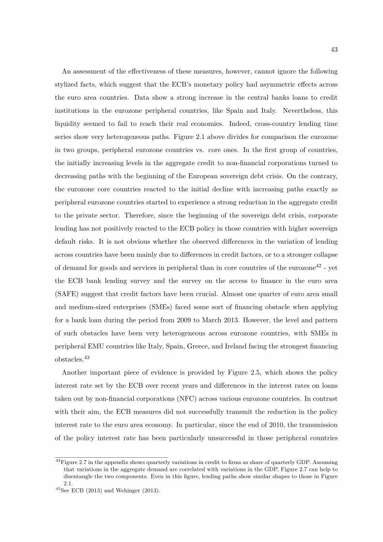
43
An assessment of the effectiveness of these measures, however, cannot ignore the following
stylized facts, which suggest that the ECB’s monetary policy had asymmetric effects across
the euro area countries. Data show a strong increase in the central banks loans to credit
institutions in the eurozone peripheral countries, like Spain and Italy. Nevertheless, this
liquidity seemed to fail to reach their real economies. Indeed, cross-country lending time
series show very heterogeneous paths. Figure 2.1 above divides for comparison the eurozone
in two groups, peripheral eurozone countries vs. core ones. In the first group of countries,
the initially increasing levels in the aggregate credit to non-financial corporations turned to
decreasing paths with the beginning of the European sovereign debt crisis. On the contrary,
the eurozone core countries reacted to the initial decline with increasing paths exactly as
peripheral eurozone countries started to experience a strong reduction in the aggregate credit
to the private sector. Therefore, since the beginning of the sovereign debt crisis, corporate
lending has not positively reacted to the ECB policy in those countries with higher sovereign
default risks. It is not obvious whether the observed differences in the variation of lending
across countries have been mainly due to differences in credit factors, or to a stronger collapse
of demand for goods and services in peripheral than in core countries of the eurozone42 - yet
the ECB bank lending survey and the survey on the access to finance in the euro area
(SAFE) suggest that credit factors have been crucial. Almost one quarter of euro area small
and medium-sized enterprises (SMEs) faced some sort of financing obstacle when applying
for a bank loan during the period from 2009 to March 2013. However, the level and pattern
of such obstacles have been very heterogeneous across eurozone countries, with SMEs in
peripheral EMU countries like Italy, Spain, Greece, and Ireland facing the strongest financing
obstacles.43
Another important piece of evidence is provided by Figure 2.5, which shows the policy
interest rate set by the ECB over recent years and differences in the interest rates on loans
taken out by non-financial corporations (NFC) across various eurozone countries. In contrast
with their aim, the ECB measures did not successfully transmit the reduction in the policy
interest rate to the euro area economy. In particular, since the end of 2010, the transmission
of the policy interest rate has been particularly unsuccessful in those peripheral countries
42Figure 2.7 in the appendix shows quarterly variations in credit to firms as share of quarterly GDP. Assumingthat variations in the aggregate demand are correlated with variations in the GDP, Figure 2.7 can help todisentangle the two components. Even in this figure, lending paths show similar shapes to those in Figure2.1.
43See ECB (2013) and Wehinger (2013).
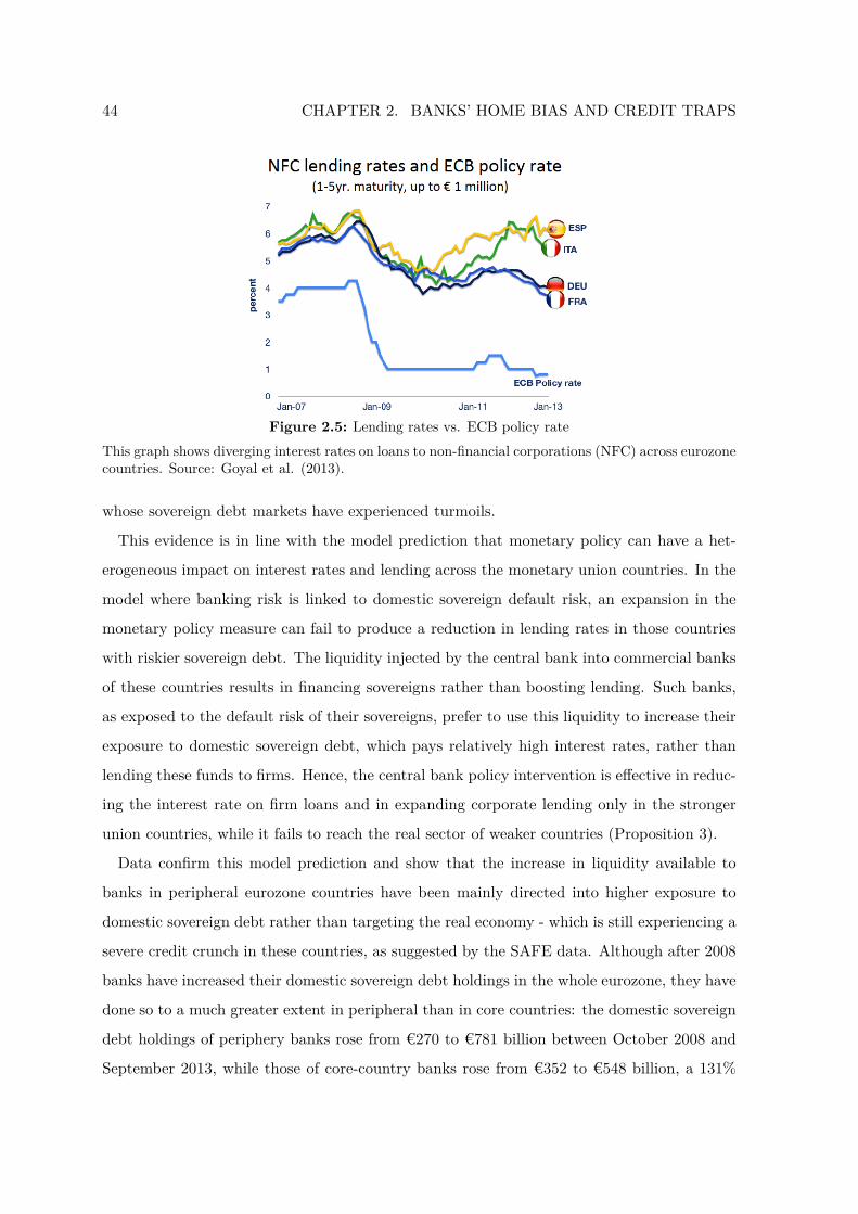
44 CHAPTER 2. BANKS’ HOME BIAS AND CREDIT TRAPS
Figure 2.5: Lending rates vs. ECB policy rateThis graph shows diverging interest rates on loans to non-financial corporations (NFC) across eurozonecountries. Source: Goyal et al. (2013).
whose sovereign debt markets have experienced turmoils.
This evidence is in line with the model prediction that monetary policy can have a het-
erogeneous impact on interest rates and lending across the monetary union countries. In the
model where banking risk is linked to domestic sovereign default risk, an expansion in the
monetary policy measure can fail to produce a reduction in lending rates in those countries
with riskier sovereign debt. The liquidity injected by the central bank into commercial banks
of these countries results in financing sovereigns rather than boosting lending. Such banks,
as exposed to the default risk of their sovereigns, prefer to use this liquidity to increase their
exposure to domestic sovereign debt, which pays relatively high interest rates, rather than
lending these funds to firms. Hence, the central bank policy intervention is effective in reduc-
ing the interest rate on firm loans and in expanding corporate lending only in the stronger
union countries, while it fails to reach the real sector of weaker countries (Proposition 3).
Data confirm this model prediction and show that the increase in liquidity available to
banks in peripheral eurozone countries have been mainly directed into higher exposure to
domestic sovereign debt rather than targeting the real economy - which is still experiencing a
severe credit crunch in these countries, as suggested by the SAFE data. Although after 2008
banks have increased their domestic sovereign debt holdings in the whole eurozone, they have
done so to a much greater extent in peripheral than in core countries: the domestic sovereign
debt holdings of periphery banks rose from €270 to €781 billion between October 2008 and
September 2013, while those of core-country banks rose from €352 to €548 billion, a 131%
45
Figure 2.6: Banks’ domestic sovereign holdingsThis graph shows the amount of sovereign debt held by domestic banks in the eurozone. Austria,Belgium, Finland, France, Germany and the Netherlands are defined as “core countries”, while Greece,Ireland, Portugal, Spain and Italy are defined as “periphery countries.” Source: Battistini, Pagano,and Simonelli (2014).
increase in the former versus a 56% increase in the latter (Figure 2.6).44
To summarize, the model mechanisms provide explanations that qualitatively fit the de-
scriptive evidence reported above. The model interpretation of such stylized facts develops
as follows. The unconventional measures adopted by the ECB can have a positive impact
on the general equilibrium interplay between liquidity, firms’ collateral values, and lending,
so they can contrast the lending reduction during an economic downturn and allow more
firms to borrow and invest. However, the exposure of eurozone banks to their home country
sovereign default risk can provide incentive for financing sovereigns more than business, and
this feature can impair the monetary transmission mechanism. Although ECB’s unconven-
tional measures have been able to circumvent the collapse in the interbank market and to
provide banks with sufficient liquidity, this policy has been insufficient to guarantee a stim-
ulus to corporate lending, especially in those eurozone economies which mainly suffer from a
credit crunch. The mere increase in the liquidity has failed to reach the real economy in the
periphery, exacerbating instead the segmentation in the eurozone sovereign debt markets and
the exposure of banks to their sovereign debt, so strengthening the non desirable dependence
of banking risk on domestic sovereign risk.
44See Battistini et al. (2014).
46 CHAPTER 2. BANKS’ HOME BIAS AND CREDIT TRAPS
2.6 Conclusion
This paper studies the limitations of unconventional monetary policy in stimulating lending
in the presence of disruptions in the financial system. The framework considered is a monetary
union which includes the eurozone banks’ exposure to domestic sovereign default risk, to study
how it affects monetary transmission and, in particular, the effectiveness of central bank’s
measures aimed at stimulating corporate lending during a crisis.
The model shows that banks’ home bias has a crucial impact on monetary policy, limiting
its effectiveness and producing heterogeneous lending responses across the monetary union
countries. The theoretical mechanism helps to understand the heterogeneous lending paths
that EMU countries have recently displayed. It also highlights a trade-off in the use of
forceful monetary policy measures. On the one hand, a strong intervention is necessary in
order to produce a relevant impact on lending in those countries who are characterized by
high sovereign default risk. On the other hand, it can exacerbate the problem of sovereign
debt market segmentation.
The mechanisms of this paper suggest that an intervention on the existing architecture of
the eurozone financial system could be needed first, to provide the central bank with effective
instruments to tackle the crisis. This intervention should be aimed at removing the link
between a country’s banking risk and the health of its public finances, but also at mitigating
the dependence of its real sector on domestic banking. An easier and cheaper cross-border
lending, indeed, would stimulate firms’ borrowing in those countries where credit conditions
are compromised by the exposure of domestic banking to high sovereign default risks. The
possibility of a banking union for the eurozone has recently started capturing the attention
of the current policy debate.45 This paper suggests that a similar reform, if able to promote
cross-border lending and in particular to remove or mitigate the existing strong link between
sovereign risk and domestic banking risk in the eurozone financial system,46 can have a crucial
positive effect on the monetary transmission mechanism and on the effectiveness of monetary
policy measures aimed at boosting corporate lending during a crisis.
45See, e.g., Beck ed. (2012), and Goyal et al. (2013) for more details.46This feature is debated. See, for instance, Acharya: “Banking union in Europe and other reforms,” in Beck
ed. (2012), which proposes to directly limit the ability of sovereigns to entangle banking system with theirdebt without advance collateralization of such debt.

47
2.7 Appendix A. Proofs
2.7.1 Proof of Lemma 1
(i) As international investors are willing to underwrite country i’s sovereign bonds at an
interest rate rgoviint = ρi1−ρi , their equilibrium interest rate rgovi cannot exceed ρi
1−ρi , ∀i. Both
countries’ banks are indifferent between lending funds to firms at an interest rate rf and
underwriting country i’s sovereign bonds, ∀i, if and only if the expected return on investments
are equal, 1 + rf = (1− ρi) (1 + rgovi) ⇔ rgovi = rf+ρi1−ρi . As rgovi ≤ ρi
1−ρi , ∀i, this condition
is never satisfied for any rf > 0. In this case firm loans guarantee a higher expected return
than government bonds, and banks supply funds to firms only. It results that, for any rf > 0,
the overall supply of funds from banks and the overall demand from firms must equal. Only
if rf = 0, the condition guaranteeing equal expected returns on government bonds and firm
loans can be satisfied, and banks can find convenient to underwrite sovereign bonds at an
interest rate equal to ρi1−ρi . Consequently, in equilibrium rgovi = ρi
1−ρi . At rf = 0, banks are
indifferent between lending to firms, depositing with the central bank, underwriting country
i’s sovereign debt at interest rate ρi1−ρi , and holding a differentiated sovereign bonds portfolio,
whose country R’s sovereign bonds share is x and country S’ sovereign bonds one is 1 − x,
with x ∈ [0, 1]. �
(ii.a) From (i), we know that country i’s banks underwrite a positive amount sovereign
debt only if ri = 0, ∀i. Then, for any aggregate liquidity L < Lmax, where Lmax is the level
for which ri = 0, the whole supply of funds can be invested into firm loans only. Assume the
aggregate liquidity is any L < Lmax, and the two markets for funds are in equilibrium for
ri > rj . If rj is the country j’s equilibrium interest rate on domestic loans, the equilibrium
interest rate on loans to foreign firms will be rj + c. Consider first the case where ri > rj + c.
Those country i’s firms whose investment PC is satisfied and whose B ≤ P1+rj+c apply for
foreign loans, all the other deposit funds in the domestic banks, with country i’s aggregate
supply of funds larger or equal to L +´ IP/(1+ri) (I −B) dF (B) > 0. No domestic no foreign
firm demands those funds, consequently ri moves down. The same argument applies at any
ri > rj + c, then in equilibrium it must be ri ≤ rj + c, at which no firm prefer to apply for
foreign loans. (Notice that ri ≤ rj + c implies that, if B > P1+ri then B > P
1+rj+c - which
means that no firm who does not have access to sufficient domestic funds to undertake the
project, can have access to sufficient foreign funds to undertake the project.) Then, there is

48 CHAPTER 2. BANKS’ HOME BIAS AND CREDIT TRAPS
no equilibrium where ri > rj + c and banks lend funds to firms abroad. �
(ii.b) The only case left to consider from (ii.a) is the one where rj < ri ≤ rj + c. From (iii)
below, we know that the investment participation constraint is always satisfied. As there is no
lending abroad, in each country the equilibrium interest rate is such that the domestic supply
of funds equals the domestic demand for funds. As ri > rj , the supply of funds in county i
= L+´ IP/(1+ri) (I −B) dF (B) > L+
´ IP/(1+rj) (I −B) dF (B) = supply of funds in country j,
while the demand for funds in county i =´ P/(1+ri)
0 BdF (B) <´ P/(1+rj)
0 BdF (B) = demand
for funds in country j. If the market for funds is in equilibrium in country j, it cannot be in
equilibrium for country i, unless ri moves down until it equals rj , level at which the market
for funds is in equilibrium in country i too. �
(iii) From (ii.a), in equilibrium no firm borrows from abroad. This implies that the interest
rate on firm loans is the same as the one on deposits, consequently the investment partic-
ipation constraint can be simplified as follows: X1[γ + (1− γ) YP
]+X2 (1− γ) ≥ I (1 + ri)
·[γ + (1− γ) YP
]. This condition defines a threshold ri in the interest rate on deposits above
which firms have no incentive to undertake the project. Notice that ri is independent of B:
either the investment participation constraint is satisfied for all firms, or it is satisfied for
no firm. Assume that r > ri. All firms deposit their initial wealth in the domestic banks.
Assuming aggregate central bank liquidity at minimum level L = 0, the total supply of funds
equals´ I
0 (I −B) dF (B) > 0. No demand for funds comes from firms and, as r > 0, no
demand for funds comes from governments. The total demand for funds is null, hence the
market does not clear, and the interest rate moves down until r ≤ ri. Assuming L > 0
increases further a supply of funds facing no demand, hence the same argument applies. �
(iv) Assume L1 > L0 and r (L1) = r (L0) = r > 0. It implies that, for L = L0, the interest
rate r is such that the supply of S (·) = L0+´ IP/(1+r)(I−B)dF (B) equals the demand of funds
D (·) =´ P/(1+r)
0 BdF (B). But then the supply of funds if L = L1, S (·) = L1 +´ IP/(1+r)(I −
B)dF (B), is larger than the supply of funds if L = L0, S (·) = L0 +´ IP/(1+r)(I − B)dF (B),
and larger than the demand of funds D (·) =´ P/(1+r)
0 BdF (B). The market for funds is not
in equilibrium, and the interest rate moves down until the demand for funds and the supply
of funds when L = L1 equal each other. Therefore, L1 > L0 ⇒ r (L1) < r (L0), ∀L ≤ Lmax,
where Lmax is the aggregate liquidity for which the interest rate reaches the zero bound. �

49
2.7.2 Proof of Proposition 1
Once obtained the results of Lemma 1, the benchmark case mechanism follows quite directly
Benmelech and Bergman (2012), with the difference that the unique collateral market across
the union countries implies that γR + γS matters for determining whether the equilibrium is
“conventional” or not.
(i) Given L and Q(Bi, ri), the equilibrium price of the asset, P (Bi, ri) = min(Q(Bi,ri)γR+γS , Y
),
increases as γR + γS reduces, until it reaches the full value Y . From Lemma 1, sufficient
increases in liquidity eventually lead the equilibrium interest rate at the zero bound. Suppose
L = Lmax, the level implying that the interest rate reaches the zero-bound. Suppose not all
firms with borrowing requirement B ≤ Y get enough funds to undertake the project. If
the total supply of asset γR + γS is low enough, then Q(Bi,ri)γR+γS > Y . This implies that the
equilibrium price of liquidated asset equals the full value, P ∗ = Y . In this case, it is optimal
for banks to lend funds to any loan applicant B ≤ P ∗ = Y at t = 0. Then, there is a
level γR + γS such that, for a sufficiently forceful liquidity injection, lending must be at the
maximum possible level:´ Y
0 BdF (B). �
(ii) Given L and Q(Bi, ri), Q(Bi,ri)γR+γS reduces as γR + γS increasing, reaching at some point
the value Y . From that point onwards, a further increase in γR + γS implies that P ∗ < Y .
Suppose L = Lmax, the level implying that the interest rate reaches the zero-bound, and
suppose all firms with borrowing requirement B ≤ Y get enough funds to undertake the
project. At t = 1, the aggregate liquidity available to firms demanding liquidated assets,
Q(Bi, ri), will be maximum. Even for this maximum possible liquidity level, however, if the
supply of asset γR+γS is too high relative to the demand, the equilibrium price of liquidated
asset can be lower than its full value, P ∗ = Q(Bi,ri)γR+γS < Y . In this case, it is not optimal for
banks to lend funds beyond P ∗ < Y at t = 0. The total lending will be at a suboptimal level,´ P ∗0 BdG(B) <
´ Y0 BdF (B), and additional liquidity injections beyond Lmax will have no
effects. The time-0 equilibrium interest rate on loans is already at the zero bound, banks will
use additional liquidity only to increase their central bank deposits or to underwrite sovereign
bonds. Therefore, there is a threshold γ such that, if γ = γ1+γ22 > γ, the equilibrium asset
liquidation value P ∗ < Y , lending is constrained to a suboptimal level, and liquidity injections
beyond Lmax do not produce further increases in corporate lending. �

50 CHAPTER 2. BANKS’ HOME BIAS AND CREDIT TRAPS
(iii) Lemma 1 shows that, independently of differences in sovereign default riskρi, for any
aggregate liquidity level the equilibrium interest rate is cross-country equal. Unique market
implies that the collateral price is cross-country equal too. It follows that corporate lending
is cross-country equal for any aggregate liquidity level. Therefore, increases in the aggregate
liquidity have exactly the same effect across the monetary union countries. �
2.7.3 Proof of Lemma 2
(i-ii) Define L the aggregate liquidity level at which rR reaches ρR1−ρR . For any L ≤ L it
is easy to verify that Lemma 1 (ii) and (iii) still apply. Therefore, the equilibrium interest
rate is the same in both countries, and there is no lending abroad. In each country, it is
not possible that the investment participation constraint is satisfied for no firm. If r > ri, it
is possible that the investment PC is satisfied for those firms whose borrowing requirement
does not exceed a certain B, while it is not satisfied for the other firms. In this case, the
borrowing requirement identifying the marginal borrowing firm is B = min(
P1+r , B
), with
the total supply of funds being equal to´ I
min( P1+r ,B) (I −B) dF (B). As by assumption ρi < ri,
governments do not demand banks’ funds, therefore the total demand for funds is equal to´ min( P1+r ,B)
0 BdF (B). As the right hand side of condition (2.14) is increasing in the interest
rate, the level of borrowing requirement B decreases as the interest rate reduces. As the
aggregate liquidity increases, supply of funds increases, the interest rate moves down. At a
certain liquidity level L the interest rate eventually reaches ri, for which the participation
constraint is satisfied for all firms. As L is the aggregate liquidity level at which the interest
rate reaches ρi1−ρi , and as by assumption ri > ρi
1−ρi , then it must be that L < L. �
(iii-iv) As L increases, at a certain level L the interest on loans reaches the level ρi1−ρi , for
which banks are indifferent between lending to firms and underwriting domestic sovereign
debt. The profit max problem (2.9), indeed, implies that corporate lending is higher than
0only if rfDi ≥ rgD . As far as the marginal buyer of sovereign debt is an international investor,
the equilibrium interest rate on sovereign bonds rgD remains constant at rgD = ρi1−ρi , and so
the interest rate on firm loans, rfDi = ρi1−ρi . Liquidity injections only increase the amount
of sovereign debt purchased by domestic bank. Only as liquidity reaches the level L, where
the marginal buyer of sovereign debt is a domestic firm, the interest rate on loans is again
reducing in the aggregate liquidity level, hence corporate lending is again increasing in the
aggregate liquidity level. As far as the sovereign default risks are cross-country different, this

51
mechanism applies at different liquidity levels for the two countries.
Notice also the role played by the constant marginal cost on foreign lending c. In equi-
librium, the possibility of cross-border lending implies that cross-country differences in the
interest rate on firm loans must lie in the interval [−c, c]. Suppose they do not, and in par-
ticular that rR > rS + c. Banks in S start to lend funds to firms in R, until the interest rates
adjust such that rR = rS + c.
As remark, note that, in the banks’ home bias scenario, the risk of bank bankruptcy
may rise the firm’s incentive not to deposit funds in the bank. The setup described in
Section 2 does not allow firms not to deposit funds. Suppose banks can deposit a share
a ∈ [0, A]. The linearity of the maximization problem guarantees that the two solution
candidates are at the borders, a = A versus a = 0. The value of the time-0 expected payoff
when a = A is given by the right hand side of equation (2.14), while a = 0 leads to a
time-0 expected payoff equal to γi (I −B + P ) + (1− γi)(I −B +X
′2
). Rearranging terms,
a = A � a = 0 ⇔ r.h.s. of equation (2.14) ≥ γi (I −B + P ) + (1 − γi)(I −B +X
′2
)⇔
rdi ≥[ρiα+ (1− ρi)
(γ + (1− γ) YP
)]−1− 1. This condition fixes a possibly larger than zero
lower bound for the equilibrium interest rate on deposit in country i. However, the maximum
possible value of this lower bound, which is reached when P ∗ = Y , is still strictly smaller
than ρi1−ρi , for any α ∈ (0, 1]. Therefore the property that, for L > L, the interest rate on
firm loans decreases in L is preserved. �
2.7.4 Proof of Proposition 2
(i-ii) In the following, I show that there is a non empty set Γ such that, for γ ∈ Γ, in the
benchmark case the economy is in a “conventional equilibrium” in both the union countries,
while in the banks’ home bias scenario, for ρi > 0, country j’s economy is in a “credit trap
equilibrium.”47
From Proposition 1, we have that a reduction in the interest rate increases lending for
a given asset liquidation price which, in turn, increases time-1 liquidity and possibly the
asset price which, in turn, increasing lending at time-0 even further. Therefore, lending
can be at the maximum level only if the aggregate liquidity is sufficiently high to lead to
zero equilibrium interest rate. Define γ0 > 0 the value for which, in the benchmark case,
at L = Lmax - where Lmax is the level such that the interest rate is at the zero bound -47“Conventional equilibrium” and “credit trap equilibrium” are defined similarly to Benmelech and Bergman
(2012).

52 CHAPTER 2. BANKS’ HOME BIAS AND CREDIT TRAPS
Q(Bi,ri)γ0
= Y , with consequently the economy being in a conventional equilibrium.
Suppose γ = γ0, and banks are home biased. Suppose we are at t = 1 and sovereign default
occurs in country i. For any liquidity injection at time-0, the time-1 aggregate liquidity
available to potential buyers of liquidated asset never exceeds the threshold Q(Bi, ri) =
Q(Bi, ri) −´ IEi[P ]/(1+ri)(I − Bi)(1 + ri)dF (Bi). The liquidity can reach this level only in
the case that lending in the previous period has been maximum, while in all the other
cases it will be lower. Suppose lending has been maximum in the previous period, which
makes the value of the integral minimum (highest lending means lowest firm deposit in the
banks). Still, the assumption that Y < I implies that´ IEi[P ]/(1+ri)(I − Bi)(1 + ri)dF (Bi) >
0, then Q(Bi, ri) < Q(Bi, ri). But then Q(Bi,ri)γ0
< Q(Bi,ri)γ0
= Y and then P (Bi, ri) =
min(Q(Bi,ri)
γ0, Y)
= Q(Bi,ri)γ0
< Y .
Country j’s banks are not bankrupt in this state of the world (it is enough that they
are not bankrupt with positive probability). If they lent funds up to Y , as the price of
the asset P ∗ < Y , there are firms who do not fully repay the loan. But then the loan
contract is not optimal, which is a contradiction. For this reason, independently of further
increases in lending at time-0, country j’s banks willingness to lend funds cannot exceed
Ej [P ] = (1− ρi)Y +ρiP∗ < Y . Therefore, at t = 0 country j’s lending cannot be maximum.
Then the country j’s economy is in a credit trap, γ0 ∈ Γ and, since γ0 > 0, Γ is a non empty
set.
Notice that the validity of this proof remains unchanged if a weaker formulation of banks’
home bias is assumed, namely, if sovereign default implies domestic banks bankruptcy only
with some probability q, with 0 < q < 1. In this alternative formulation, it is possible to
similarly show the existence of a non empty set Γ′ such that, for γ ∈ Γ′ , in the benchmark
case the economy is in a “conventional equilibrium” in both the union countries, while in the
banks’ home bias scenario, for ρi > 0, country j’s economy is in a “credit trap equilibrium.”
The only difference is that Γ′ ⊆ Γ. �
(iii) Trivial, given the proof of (i-ii) and Lemma 2. �
2.7.5 Proof of Proposition 3
I provide the proof for the case where ρR > ρS = 0. The logic rather straight extends to
the more general case where ρR > ρS ≥ 0 which is also considered in Proposition 3.
In country S, increases in liquidity continuously reduce the interest rate on firm loans
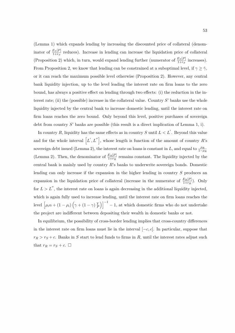
53
(Lemma 1) which expands lending by increasing the discounted price of collateral (denom-
inator of ES [P ]1+rS reduces). Increase in lending can increase the liquidation price of collateral
(Proposition 2) which, in turn, would expand lending further (numerator of ES [P ]1+rS increases).
From Proposition 2, we know that lending can be constrained at a suboptimal level, if γ ≥ γ,
or it can reach the maximum possible level otherwise (Proposition 2). However, any central
bank liquidity injection, up to the level leading the interest rate on firm loans to the zero
bound, has always a positive effect on lending through two effects: (i) the reduction in the in-
terest rate; (ii) the (possible) increase in the collateral value. Country S’ banks use the whole
liquidity injected by the central bank to increase domestic lending, until the interest rate on
firm loans reaches the zero bound. Only beyond this level, positive purchases of sovereign
debt from country S’ banks are possible (this result is a direct implication of Lemma 1, i).
In country R, liquidity has the same effects as in country S until L < L′ . Beyond this value
and for the whole interval[L′, L′′], whose length is function of the amount of country R’s
sovereign debt issued (Lemma 2), the interest rate on loans is constant in L, and equal to ρR1−ρR
(Lemma 2). Then, the denominator of ER[P ]1+rR remains constant. The liquidity injected by the
central bank is mainly used by country R’s banks to underwrite sovereign bonds. Domestic
lending can only increase if the expansion in the higher lending in country S produces an
expansion in the liquidation price of collateral (increase in the numerator of ER[P ]1+rR ). Only
for L > L′′ , the interest rate on loans is again decreasing in the additional liquidity injected,
which is again fully used to increase lending, until the interest rate on firm loans reaches the
level[ρiα+ (1− ρi)
(γ + (1− γ) YP
)]−1− 1, at which domestic firms who do not undertake
the project are indifferent between depositing their wealth in domestic banks or not.
In equilibrium, the possibility of cross-border lending implies that cross-country differences
in the interest rate on firm loans must lie in the interval [−c, c]. In particular, suppose that
rR > rS + c. Banks in S start to lend funds to firms in R, until the interest rates adjust such
that rR = rS + c. �
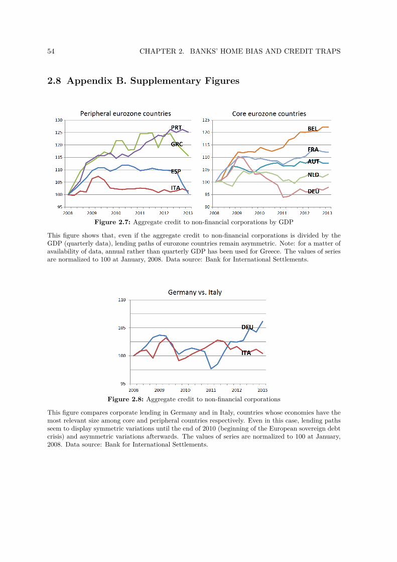
54 CHAPTER 2. BANKS’ HOME BIAS AND CREDIT TRAPS
2.8 Appendix B. Supplementary Figures
Figure 2.7: Aggregate credit to non-financial corporations by GDP
This figure shows that, even if the aggregate credit to non-financial corporations is divided by theGDP (quarterly data), lending paths of eurozone countries remain asymmetric. Note: for a matter ofavailability of data, annual rather than quarterly GDP has been used for Greece. The values of seriesare normalized to 100 at January, 2008. Data source: Bank for International Settlements.
Figure 2.8: Aggregate credit to non-financial corporations
This figure compares corporate lending in Germany and in Italy, countries whose economies have themost relevant size among core and peripheral countries respectively. Even in this case, lending pathsseem to display symmetric variations until the end of 2010 (beginning of the European sovereign debtcrisis) and asymmetric variations afterwards. The values of series are normalized to 100 at January,2008. Data source: Bank for International Settlements.

55
Figure 2.9: Home share of sovereign debt held by banks (2011)This graph shows the fraction of sovereign debt held in the form of domestic sovereign debt, aggregatingin each country across the banks in the data sample used by the European bank stress test in 2011.Source: Uhlig (2013).


Chapter 3
Labor Market Frictions and Fertility

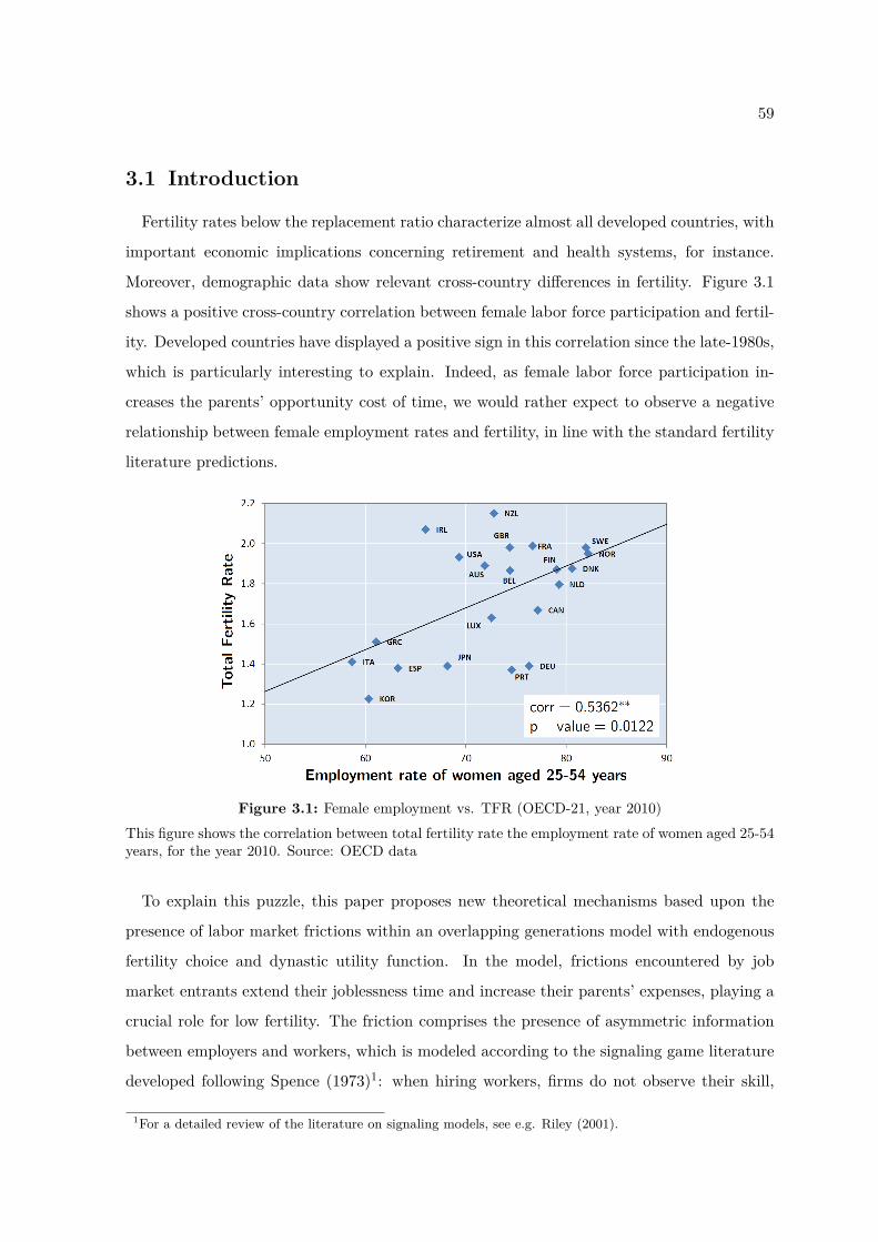
59
3.1 Introduction
Fertility rates below the replacement ratio characterize almost all developed countries, with
important economic implications concerning retirement and health systems, for instance.
Moreover, demographic data show relevant cross-country differences in fertility. Figure 3.1
shows a positive cross-country correlation between female labor force participation and fertil-
ity. Developed countries have displayed a positive sign in this correlation since the late-1980s,
which is particularly interesting to explain. Indeed, as female labor force participation in-
creases the parents’ opportunity cost of time, we would rather expect to observe a negative
relationship between female employment rates and fertility, in line with the standard fertility
literature predictions.
Figure 3.1: Female employment vs. TFR (OECD-21, year 2010)This figure shows the correlation between total fertility rate the employment rate of women aged 25-54years, for the year 2010. Source: OECD data
To explain this puzzle, this paper proposes new theoretical mechanisms based upon the
presence of labor market frictions within an overlapping generations model with endogenous
fertility choice and dynastic utility function. In the model, frictions encountered by job
market entrants extend their joblessness time and increase their parents’ expenses, playing a
crucial role for low fertility. The friction comprises the presence of asymmetric information
between employers and workers, which is modeled according to the signaling game literature
developed following Spence (1973)1: when hiring workers, firms do not observe their skill,
1For a detailed review of the literature on signaling models, see e.g. Riley (2001).

60 CHAPTER 3. LABOR MARKET FRICTIONS AND FERTILITY
although workers can invest in costly education to signal it. The idea behind job market
signaling models is that workers entering the labor market undertake most of their actions
not only to increase their ability, but also to signal their skill. The costly signal not only
interprets education investment, but also any other costly qualification that a worker would
include in his/her résumé to signal his/her skill when applying for a job.
The presence of asymmetric information leads, in equilibrium, to high-skill agents optimally
deciding to invest time in education before entering the labor market to separate themselves
from low-skill workers and receive a better wage. A first effect on fertility is straightforward:
the higher the education investment, the less the time and income available for child-rearing.
Moreover, the dynamic structure of the model allows capturing a second, forward-looking
effect. Suppose that children are financially dependent on their parents during their jobless-
ness period. Parents who care about their children may want to support them until they find
a job; thus, the children’s education investment choice will affect the expenses that parents
face. In other words, it will affect the child cost and consequently the parents’ fertility choice.
What is the effect of better education on fertility? It is reasonable to assume that a better
education system is more effective in terms of both (i) increasing human capital and (ii)
ranking people and signaling their skill. For simplicity, in line with the signaling literature,
the model does not consider the first feature, rather focusing only on the second.2
Suppose that a better education system makes it more difficult for bad students to obtain
good grades. As higher educational attainments are more difficult to achieve for low-skill
agents, their incentives to undertake the path eventually leading to high-skill jobs reduce.
Therefore, in countries where education and labor market institutions are better, it will be
easier and faster for high-skill workers to reach such positions. In other words, the inefficiency
produced by asymmetric information is lower, as workers can more easily signal their ability
to firms, so the labor force allocation works more rapidly and more efficiently.
The model exploits the aforementioned mechanism to analyze the impact on fertility of
cross-country differences in the quality of education and labor market institutions, finding
that a better “signal technology” positively influences fertility in two ways: first, having a
family with children becomes more affordable, since young adults start to work earlier and
their income is higher; and second, parents need to support their children for a shorter period
of time, as they manage to find a job earlier and hence the child cost reduces. Therefore,
2Appendix C.III briefly discusses the robustness of the main results to a different model specification whereeducation is human capital increasing.

61
countries with better education and labor markets will display higher youth labor force par-
ticipation and higher fertility.
Nevertheless, the model can still allow for the negative within-country relationship between
income and fertility that characterizes developed countries. Indeed, even in those economies
where the signal technology is better, high-skill agents invest in education more than their
low-skill counterparts, trading a higher wage off against less time for child-rearing. For this
reason and the higher opportunity cost of their time, high-wage workers’ fertility can result
in being lower compared with low-wage workers.
As the asymmetric information problem considered here arises in the transition from edu-
cation to work, not only the quality of education but also the labor regulation matters for the
severity of the friction incidence. Therefore, a model extension explicitly considers differences
in labor regulation as an additional source of potential differences in fertility. I find that a
regulation excessively constraining job contract renegotiation depresses fertility similarly as
an inadequate signal technology does. Limiting renegotiation can raise the ex-ante incen-
tives for low-skill agents to apply for jobs requiring high skills. High-skill workers will need
to over-invest in education to reveal their true type and their joblessness time will extend.
Thus, in countries with excessive labor market rigidities, young workers will have less time
and the income to spend in child-rearing, and fertility will be lower.
Several proxies for the quality of education and labor market concerning developed coun-
tries and particularly European countries seem to confirm the presence of a link between
fertility and education and labor market characteristics across countries. In particular, we
observe negative correlations between measures of the incidence of labor market frictions and
fertility rates. Section 4 interprets my findings in the light of the empirical evidence, showing
that the model predictions qualitatively fit the data.
During recent decades, a large body of literature has investigated the issue of low fertility
facing raising income in developed countries. Based upon the seminal works by Becker (1960,
1965), Mincer (1962, 1963) and Becker and Lewis (1973), the main argument of the standard
theory develops as follows. As raising children entails a cost, mostly in terms of time, the
secular increase in income and female earning power increased the opportunity cost of parental
time, making childbearing more expensive and lowering fertility rates.3 Another common
3Actually, some of these theories are not as robust as commonly believed, in the sense that several specialassumptions are needed to generate the negative relationship: for a detailed discussion of this issue and amore complete survey of the literature, see e.g. Jones, Schoonbrodt, and Tertilt (2010).

62 CHAPTER 3. LABOR MARKET FRICTIONS AND FERTILITY
argument in the literature is that higher-income people have a higher demand for child quality,
making quantity more costly. Hence, those parents prefer having fewer offspring.
However, limiting the analysis to this substitution effect would leave unexplained the ob-
served positive correlation between female participation rates and fertility across developed
countries. Indeed, Ahn and Mira (2002) already underlined the inconsistency with data of
Butz and Ward (1979), the mainstream empirical model built on the theoretical results of
the standard fertility literature. According to this model, we should have observed a cross-
country negative correlation between female participation rates and fertility, becoming more
negative with the increase of female labor force participation over time. OECD data display
exactly the opposite, suggesting that there is a gap in the fertility theory, which this papers
aims to fill.
In line with the ideas formalized by this paper, some recent empirical works hypothesize
that labor market features can play a crucial role in explaining cross-country differences in
fertility, e.g. Adserà (2004, 2005, 2006) and the above-mentioned Ahn and Mira (2002).
Da Rocha and Fuster (2006) quantitatively study a closely related research question,
namely the role of unemployment in generating the observed positive association between
fertility and female employment among OECD countries. They find that unemployment in-
duces women to postpone and space births, which result in lower fertility.4 By contrast,
my aim is to analyze how differences in the labor market micro-structure can endogenously
produce differences in young workers’ conditions and ultimately in their fertility decisions.
Related to my paper, Sommer (2011) finds that rising income uncertainty reduces fertil-
ity. Young households postpone childbearing when income uncertainty is high, preferring to
work and accumulate more precautionary savings before starting a family. In the presence of
infertility risk increasing over age, the birth postponement reduces fertility. The mechanism
is based upon the idea developed by Chetty and Szeidl (2007) that income uncertainty has
a negative effect on consumption commitments: when earnings shocks become larger, agents
are less willing to commit to children. Santos and Weiss (2011) exploit quantitatively a sim-
ilar argument, albeit analyzing the delay in marriage. However, the mechanism highlighted
in these papers does not seem convincing in terms of explaining fertility differences across
countries. Labor earning volatility over has been higher in the US than in Europe in recent
4However, at least Italy - whose unemployment has been closer to the European average over recent decades,while fertility has been constantly lower - seems to provide a counterexample to their findings. On thecontrary, the evidence considered in Section 4 below shows a large incidence of frictions in the Italian labormarket, which may have depressed fertility as suggested by the theoretical channels exploited here.

63
decades,5 although fertility rates have also been higher.6
Finally, Manuelli and Seshadri (2009) provide an alternative explanation of cross-country
differences in fertility from what I propose here, omitting labor market frictions. They incor-
porate human and health capital in the Barro-Becker (1989) model to explore how economic
forces affect fertility and mortality across countries, finding that differences in productivity
and taxes can play an important role in generating the observed differences in fertility and
mortality between Europe and the US.
The remainder of this paper is structured as follows. In Section 2, I present the model
setup. In Section 3, I characterize the equilibrium of the economy and describe the effect of
labor market frictions on fertility. Section 4 analyzes the model predictions by comparison
with the empirical evidence, and Section 5 concludes.
3.2 Model Setup
The economy is populated by overlapping generations of agents who live for three periods
- namely as children, young adults and old adults - and by identical firms that behave com-
petitively. For simplicity, I do not model gender heterogeneity; therefore, the agents can be
considered as unitary households where parents make joint decisions.
In each period, there is a continuum of measure 1 of young adults, ex-ante heterogeneous
in skill, high (θH) or low (θL). The share of high-type agents is α, with 0 < α < 1, known and
exogenously given. Children neither enjoy any utility nor take any decisions. Young adults
decide on their consumption, education, number of children and supply labor. Old adults
are no longer fertile. They supply labor, deciding on their consumption and how much to
possibly transfer to each of their children.
For simplicity, production technology only uses labor as input. Agents can still save and
borrow7 thanks to a risk-free technology, which returns 1 + r in the next period for any unit
of consumption saved.8
5According to Venn (2011), for instance, the US economy has experienced a relatively high earnings volatilityincrease over time compared to the other OECD countries.
6On the contrary, the US have been constantly characterized by lower youth unemployment and a shorterschooling-to-work transition. Therefore, labor market frictions seem more promising than consumptioncommitments to explain fertility differences between Europe and the US.
7Young agents, however, are borrowing constrained until they start working. See the agents’ problem below.8As the firms’ technology is linear, this setup is equivalent to a model where capital linearly enters the firms’production function, with constant marginal product equal to r .

64 CHAPTER 3. LABOR MARKET FRICTIONS AND FERTILITY
3.2.1 Agents’ Problem
Consider the decision problem of the young adults. The preferences are modeled by using
an extended version of the dynastic utility function introduced by Barro and Becker (1988).
Young adults differ in skill, θH or θL, although this difference does not affect their preferences.
Adults value their own consumption and discount future utility of their children. In line with
the literature, the discount factor decreases with the number of children: in other words, the
more children, the smaller the weight in discounting the future utility of an additional child.
The utility of a young adult of any type who consumes c1 in the first period and c2 in the
second period and has n children, α of which are skilled,9 is given by:
u(c1) + βu(c2) + βλn1−η(αV
′H(TH) + (1− α)V ′L(TL)
), (3.1)
where 0 < β < 1, 0 < η < 1, λ > 0, and u(·) satisfies the Inada conditions. The parameter
β is the time discount factor, λ measures the degree of parents’ altruism, η is the elasticity
of altruism with respect to the number of children, V ′H and V ′L are the utility that her skilled
and unskilled children will enjoy as adults, respectively, increasing in the respective transfers
TH and TL that they will receive, with Ti ≥ 0.
The budget constraint of the utility maximization problem of a type θ young adult is
derived as follows. In each period, the agent is endowed with one unit of time. As a young
adult, he/she can allocate his/her time between investing in education and working. For
simplicity, and without loss of generality, I assume that education costs time only.10 To
obtain a level of education equal to s, a young adult of type θ has to invest a fraction τ(s | θ)
of the total time available. In line with the signaling game literature, I make the following
assumptions concerning the signal cost function:
Assumption 1
1. The cost function τ(s | θ) is continuous, positive and convex: (i) τ(0 | θ) = 0, (ii)
τ ′(s | θ) > 0, ∀s > 0, and (iii) τ ′′(s | θ) > 0, ∀s > 0.
2. The cost function satisfies single crossing: τ ′(s | θL) > τ ′(s | θH), ∀s > 0.
The first point imposes standard regularity conditions on the signal cost function. The9In line with the literature, I assume - for simplicity - that n ∈ R+: see, e.g. Barro and Becker (1988, 1989).For a case with children heterogeneous in skill, see, e.g. Doepke (2004).
10Adding a monetary education cost t(s | θ) would not change the model results, as far as the same conditionslisted in Assumption 2 for τ(·) would also be satisfied for t(·).

65
second condition - so-called “single crossing” - is also commonly used in the literature and
imposes that an additional unit of education costs less to a high-type agent thana low-type
one, for any level of education.
Raising a child costs ρ > 0 units of consumption, independent of the parent’s type. I
do not include a time cost of child-rearing in the baseline model, as doing so simplifies the
tractability of the existence of the equilibrium on the job market. In the next section, I relax
this assumption and show that - in a simplified setting - the main mechanisms are robust to
the introduction of a time cost of child-rearing and, moreover, consistent with the observed
negative within-country correlation between income and fertility.
The budget constraint of a young adult of type θ can be represented as follows:
c1 + c21 + r
+ n
(ρ+ αTH + (1− α)TL
1 + r
)≤(
1− τ(s | θ) + 11 + r
)w(s) + T−1,θ. (3.2)
The right-hand side constitutes the agent’s wealth, comprising the current wage net of the
time invested in education, the discounted future wage and the transfer received from his/her
parent, where the −1 index means that the variable have been set by his/her parent in the
previous period. On the left-hand side are current and discounted future consumption, the
child-rearing costs and the discounted future transfers, possibly dependent on the child’s
type.
Note that the constraint (3.2) allows agents to freely borrow or save thanks to the presence
of a risk-free technology that returns 1 + r for any unit of capital invested. However, I want
to capture the notion that a young adult can be financially dependent on his/her parents
until he/she starts working.11 For this purpose, I assume that a young adult - for the time
that he/she is joblessness, τ(s | θ) - is borrowing constrained and has an instantaneous
minimum consumption level ϕ,12 which needs to be financed with a voluntary transfer from
his/her parent, T−1,θ. Therefore, the utility maximization problem also includes the following
constraint:
ϕ · τ(s | θ) ≤ T−1,θ. (3.3)
An insufficient level of the parental transfer would constrain the young agent’s education
11Besides its realism, modeling this feature allows considering another dimension along which to analyze themodel predictions by comparison with the empirical evidence, as discussed in Section 4.
12Alternatively, ϕ can be interpreted as a monetary cost of a time unit of education that borrowing constrainedstudents can only pay thanks to the parental transfer.

66 CHAPTER 3. LABOR MARKET FRICTIONS AND FERTILITY
investment, forcing him/her to start working earlier than desired.13
3.2.2 Job Market Environment
A crucial feature of the model feature is asymmetric information between firms and job
market entrants, whereby firms do not observe workers’ skill, but only the level of signal that
they choose. Asymmetric information leads to a signaling game played by young agents and
firms, which is embedded in the general equilibrium framework described above and has the
following time structure:
Timing of the Job Market
1. A random move of Nature determines the agents’ type, which is private information.
2. Having become a young adult, each agent chooses a signal level s ∈ S ⊆ R+ contingent
on his/her type and his/her parent’s type.14 The signal costs τ(s | θ) time units, with
0 ≤ τ(s | θ) ≤ 1.
3. For each agent, firms observe s, then simultaneously make wage offers w(s).
4. The agent decides which offer to accept, if any.
5. In case of acceptance, the firm decides whether to employ the worker as a skilled or
unskilled laborer, LS or LU respectively.
The game structure is very similar to the version of the Spence (1973) signaling game
as developed e.g. in Mas-Colell, Whinston, and Green (1995) (MWG).15 The two main
modifications are that: (i) firms not only set the wage but also decide how to employ hired
workers, as discussed in further detail below; and (ii) the education signal costs time rather
than consumption good.
13This constraint is a simplification to overcome the discrete-time structure of the model not allowing for adirect representation of the hypothesized form of youth financial dependence on parents. A more directrepresentation would be possible in a slightly modified problem, where agents maximize:
τ(s | θ)u(c1,1) + (1− τ(s | θ))u(c1,2) + βu(c2) + βλn1−η(αV
′H(TH) + (1− α)V
′L(TL)
).
In this alternative formulation, the agent’s second period of life is divided into two parts, the first of whichis devoted to education and the second to working, whereby their length depends on the education choice.Subsequently, the constraint imposes that c1,1 is (i) no smaller than ϕ and (ii) no larger than the parentaltransfer. As a matter of consistency with a fully discrete-time OLG model, and for tractability reasons, thebaseline model setup uses the more standard formulation of the utility maximization problem describedabove, which can still capture the hypothesis that joblessness young agents are financially dependent ontheir parents, thanks to the constraint (3.3).
14The signal is possibly contingent on the parent’s type, as the parental transfer T−1,θ (θ−1) can constrain thesignal choice made by the agent.
15See chapter 13.C.

67
3.2.3 Technology
The single consumption good in the economy is produced by m ≥ 2 identical firms that be-
have competitively. They share a common linear technology using skilled (LS) and unskilled
(LU ) labor as inputs. Firms hire workers on the job market, setting wages competitively and
deciding how to employ the worker in case of acceptance. Moreover, the following assumption
is made:
Assumption 2
1. Each high-skill worker produces a marginal product equal to θH if employed as a skilled
laborer, LS, but produces a marginal product equal to θL if employed as an unskilled
laborer, LU .
2. Each low-skill worker produces a marginal product equal to θL if employed as an un-
skilled laborer, LU , but produces a marginal product equal to γ, with γ ≤ θL, if employed
as a skilled laborer, LS.
Given Assumption 2, the total production function of this economy can be written as
follows:
Yt = θL(LHU,t + LLU,t) + θH(LHS,t + γ
θHLLS,t),
where LiU,t is the ratio of type i workers employed as unskilled laborers over the total mass
of workers at time t, and LiS,t is the ratio of type i workers employed as skilled laborers over
the total mass of workers at time t.
Note that the standard signaling game does not consider the firms’ decision on how to
employ workers. The standard two-type signaling game would be equivalent to the setup
described above by assuming that: (i) high-ability workers always produce θH regardless of
whether they are employed as LS or LU ; and (ii) low-ability workers employed as LS produce
marginal product γ that equals θL.
Once the production involves different jobs being performed, it is clear that the assumptions
made here are not more restrictive than those made in the standard signaling game. This
setup can actually allow for a more realistic description of the hiring and working process if
one believes that the contribution of an employee depends not only on his/her ability, but
also on the job that he/she is performing.
Below, I further assume that γ takes a value strictly smaller than θL: in other words, a
low-skill worker who is performing the high-skill job produces less than he/she would have

68 CHAPTER 3. LABOR MARKET FRICTIONS AND FERTILITY
produced as an unskilled laborer.16 The following example allows better considering the
meaning of this further assumption. Suppose a company is erecting a building. Besides
construction workers, the company needs to employ engineers and surveyors. The standard
assumption of the signaling literature would imply that an engineer always produces the
same, regardless whether he/she is employed as an engineer or a surveyor, while a surveyor
always produces the same, regardless whether he/she is employed as a surveyor or an engineer.
However, it is more likely that a surveyor employed as an engineer produces a loss - probably
the collapse of the building - rather than producing as much as if performing his/her job. At
the same time, it is unlikely that an engineer employed as a surveyor will produce more than
a surveyor. That is essentially what Assumption 2 and γ < θL imply.
3.2.4 Definition of the Equilibrium
The definition of a competitive equilibrium for the economy is described as follows.
In equilibrium:
1. Every agent of any type θ ∈ Θ = {θH , θL} sets consumption c, number of children n and
transfers TL and TH , to maximize the objective function (3.1) subject to the constraints
(3.2) and (3.3).
2. The optimal education level s∗ (θ, T−1,θ (θ−1)), for any agent of type θ ∈ Θ with parent
of type θ−1 ∈ Θ, and the optimal wage schedule w∗(s), for any education level s ∈
S characterize a Perfect Bayesian Equilibrium (PBE), which requires the following
conditions to be satisfied:
(i) the worker’s strategy is optimal given the firm strategies;
(ii) the belief function µ(s) ∈ [0, 1] is derived from the worker’s strategy using Bayes’
rule where possible; and
(iii) the firms wage offers following each choice s constitute a Nash equilibrium of the
simultaneous-move wage offer game in which the probability that the worker is of
high ability is µ(s).
3. Moreover, the PBE emerging in the job market satisfies the belief refinement H defined
below. 17
16As discussed in further detail below, this assumption allows using a less strong and more intuitive equilibriumrefinement. Moreover, it simplifies the proof of Proposition 2.
17The belief refinement H is formally defined in Appendix A.

69
Note that the equilibrium defined above is recursive. Fertility does not affect the income
of future generations, owing to the simplifying assumption of linear technology, whereby
marginal products and wages are independent of the number of workers employed. Nev-
ertheless, the parental transfer can constrain the education choice of the next generation,
consequently affecting those workers’ future income.
It is well known that signaling games lead to multiple equilibria, some of which are “less
reasonable” outcomes than others. For this reason, a large body of literature has developed
to provide new equilibrium concepts that are considered more appropriate than the PBE for
signaling games. Some of these equilibrium refinements, such as the “Intuitive Criterion”
proposed by Cho and Kreps (1987), are quite intuitive and reasonable; therefore, they are
well-accepted and largely used by the following literature.18
In the setup proposed here, a very weak and intuitive refinement concept - defined e.g. in
MWG 13.AA.2 - is sufficient to obtain the uniqueness of the equilibrium. This refinement
concept is even less restrictive than the Intuitive Criterion. As a matter of convenience, it is
formally defined in Appendix A below.
The way in which this refinement concept selects among equilibria can be considered as
follows. As remarked above, in the job market game, firms do not observe the workers’
type, but rather only their education choice. In any PBE, a firm setting wage and the
employment of a worker whose education level is s attaches some probability that the worker
is of type θ - the so-called belief function µ(θ | s). The PBE concept imposes restrictions on
the firm’s belief function, which still allows for unreasonable firms’ beliefs. For this reason,
unreasonable outcomes can be supported as PBE. Instead, the refinement H imposes that
the belief function µ(θ | s) can assume values larger than zero only if there is no equilibrium
action s′ for a worker of type θ that - even in the worst possible equilibrium outcome - gives
him/her a higher wage than playing s. Otherwise, a worker of type θ would always prefer
to play s′ rather than s, since it ensures a higher equilibrium payoff: in other words, s is
equilibrium dominated for any worker of type θ. The firms knows this and consequently adjust
their belief function by attaching zero probability to the event that the signal observed s can
be a choice made by a worker of type θ, µ(θ | s) = 0.
18To obtain a unique equilibrium in the standard two-type signaling game, it is necessary to use - at least:obviously, there are stronger refinements also leading to a unique equilibrium - the Intuitive Criterion,which implies the refinement used here, subsequently imposing additional restrictions on the equilibriumfirms’ beliefs and workers’ strategies.

70 CHAPTER 3. LABOR MARKET FRICTIONS AND FERTILITY
3.3 Results
This section discusses the results of the paper. Proposition 1 characterizes the equilibria
emerging on the job market.19 Proposition 2 characterizes the main result, namely the effects
that differences in the incidence of labor market friction have on the equilibrium fertility rate.
3.3.1 Job Market Equilibrium: Characterization
The following proposition uses the results obtained in Lemma 1 (see Appendix B.I.1) to
characterize the unique job market equilibrium surviving the refinement H, as well as the
other perfect Bayesian equilibria that the game exhibits.
Proposition 1 Assume that γ < θL− α1−α (θH − θL). Under Assumptions 1 and 2, and the
conditions under which Lemma 2 holds, the game described is characterized by:
1. A unique PBE that survives the belief refinement H, in which s∗(θL) = 0, s∗(θH) = s,
w∗(s) =
θL, for s ∈ [0, s)
θH , for s ∈ [s,∞)2. PBE that do not survive the refinement H, in particular:
(i) a continuum of separating PBE, in which s∗(θL) = 0, s∗(θH) = s ∈ [s, s], w∗(s) = θL, for s ∈ [0, s)
θH , for s ∈ [s,∞)
(ii) a unique pooling PBE, in which s∗(θi) = 0, ∀i ∈ {H,L}, and the firms offer w∗(s) =
θL, ∀s.
Proof See the appendix.
The continuum of separating PBE are the same emerging in the standard version of the
Spence’s signaling game, as described in MWG 13.C. However, in contrast to the standard
game, in this job market game: (i) there is a unique pooling PBE; (ii) the refinement H
- weaker than the Intuitive Criterion and other commonly used refinement concepts - is
sufficient to obtain a unique outcome.
19For convenience, Proposition 1 is derived assuming that the constraint (3.3) in the young adults’ optimizationproblem is not binding, or it is binding at the unconstrained optimum signal; namely, the transfer that ayoung adult receives from his/her parent is sufficiently large not to constrain him/her to a certain educationlevel lower than his/her optimal choice. Then Lemma 2 provides sufficient conditions under which thisassumption is actually satisfied. Appendix C.I discusses the case in which Lemma 2 does not apply.

71
Figure 3.2: The least cost separating equilibrium
These differences are due to the fact that firms here also choose how to employ workers, as
well as the use of Assumption 2. In further detail, the reason why there is a unique pooling
PBE is as follows. By construction, in a pooling equilibrium the workers’ type is not revealed.
If a firm wants to employ workers as skilled laborers, it has to randomly choose them. For
γ sufficiently small - namely for a sufficiently small value of the low-type worker’s marginal
product, when employed as a skilled laborer - a random assignment of workers to the skilled
job is not optimal; instead, firms will optimally employ any worker as an unskilled laborer.
This implies that any worker will produce a marginal product equal to θL. The only wage
schedule consistent with the Bayes’ rule assigns the low wage to all workers, regardless of
the signal choice. Thus, in the only possible pooling equilibrium, any worker of any type
optimally chooses s = 0 and obtains the low wage.
Concerning the second point, in the standard two-type signaling game the refinement H
already rules out all the separating PBE but the least cost one. However, it does not rule out
all the pooling equilibria, rather only those in which high-type workers’ payoff is lower than
in the least cost separating outcome.20 Here, the only pooling PBE of the game is always
dominated - for high-type workers - by the least cost separating outcome. It follows that the
refinement H is sufficient to rule out all the equilibria but the least cost separating one, and
subsequently it is sufficient to obtain a unique outcome.
The unique equilibrium surviving the refinement is represented in Figure 3.2. In this
20See MWG 13.A, p. 469 ff.

72 CHAPTER 3. LABOR MARKET FRICTIONS AND FERTILITY
equilibrium - known in the literature as the least cost separating equilibrium or the Riley’s
outcome - all the high-type workers choose a signal level just sufficient to separate themselves
from the low-type workers, their true type is revealed and firms offer them a job as skilled
laborers, paying the high wage. All low-type workers choose instead not to invest in education,
their true type is revealed and firms offer them a job as unskilled laborers, paying the low
wage.21
Lemma 1 and Proposition 1 are derived assuming that the constraint (3.3) in the young
adults’ optimization problem is not binding, or it is binding at the unconstrained optimum
signal. Actually, young adults can be ex-ante constrained to a certain education level lower
than their optimal choice s∗(θ) if the transfer that they receive from their parents is not suffi-
ciently large. The following lemma provides sufficient conditions under which this possibility
is ruled out.
Lemma 2 Assume that consumption and children are normal goods. Moreover, assume
that - in the problem with homogeneous children - the elasticity of substitution with respect
to the number of children η and the child-rearing cost ρ are such that:
1− η(1 + r)ρ <
dV ′(T )/dTV ′(T ) |T=0,
where V ′ is the child’s future utility. Then there is a threshold wU in the low wage such that,
for wU ≥ wU , for any parent’s and children’s type, the constraint (3.3) in the young adults
problem is not binding, or it is binding at the unconstrained optimum s∗(θ).
Proof See Appendix B.I.3.
In equilibrium, the constraint (3) only matters for the high-type agents and never binds
low-type agents’ choice, since they always choose not to invest in education. Only if a parent
gives a transfer to his/her high-type children smaller than ϕτ(s∗(θH) | θH) will the constraint
(3) bind their education choice, and they will be unable to reach s∗(θH), the education level
necessary to reveal their true skill. Firms will employ them as unskilled laborers regardless of
their education choice, so they find it optimal not to invest in education and to start working21A technical remark is needed about the time-consistency of this equilibrium. A similar game with a time-
cost of signal may exhibit no separating equilibria when played over continuous time, if all of the followingconditions hold together: (i) the age of any worker and the moment in which he/she started education areperfectly observable; (ii) education is a continuous choice; and (iii) agents and firms have no possibility ofcommitment. However, as time is discrete in the OLG model considered, all the decision variables are setat the beginning of the period; subsequently, no time inconsistency problem arises. This issue is discussedin further detail in the proof of Proposition 1, Appendix B.I.2.
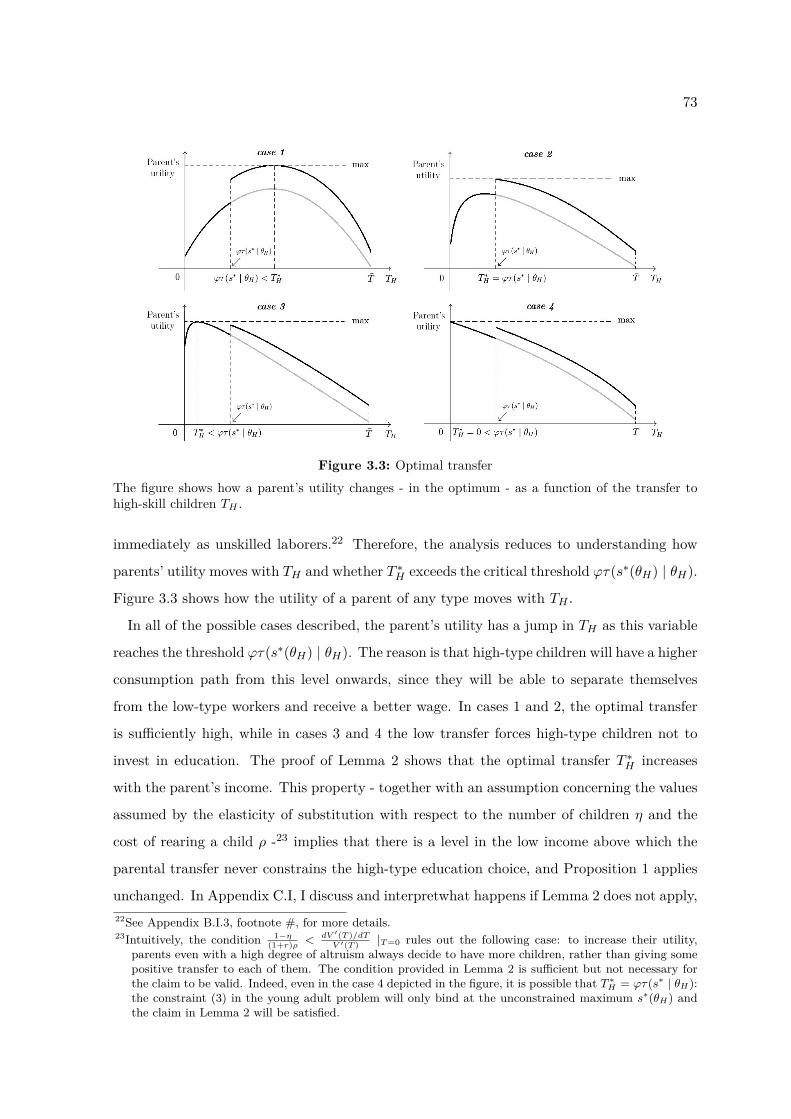
73
Figure 3.3: Optimal transferThe figure shows how a parent’s utility changes - in the optimum - as a function of the transfer tohigh-skill children TH .
immediately as unskilled laborers.22 Therefore, the analysis reduces to understanding how
parents’ utility moves with TH and whether T ∗H exceeds the critical threshold ϕτ(s∗(θH) | θH).
Figure 3.3 shows how the utility of a parent of any type moves with TH .
In all of the possible cases described, the parent’s utility has a jump in TH as this variable
reaches the threshold ϕτ(s∗(θH) | θH). The reason is that high-type children will have a higher
consumption path from this level onwards, since they will be able to separate themselves
from the low-type workers and receive a better wage. In cases 1 and 2, the optimal transfer
is sufficiently high, while in cases 3 and 4 the low transfer forces high-type children not to
invest in education. The proof of Lemma 2 shows that the optimal transfer T ∗H increases
with the parent’s income. This property - together with an assumption concerning the values
assumed by the elasticity of substitution with respect to the number of children η and the
cost of rearing a child ρ -23 implies that there is a level in the low income above which the
parental transfer never constrains the high-type education choice, and Proposition 1 applies
unchanged. In Appendix C.I, I discuss and interpretwhat happens if Lemma 2 does not apply,22See Appendix B.I.3, footnote #, for more details.23Intuitively, the condition 1−η
(1+r)ρ < dV ′(T )/dTV ′(T ) |T=0 rules out the following case: to increase their utility,
parents even with a high degree of altruism always decide to have more children, rather than giving somepositive transfer to each of them. The condition provided in Lemma 2 is sufficient but not necessary forthe claim to be valid. Indeed, even in the case 4 depicted in the figure, it is possible that T ∗H = ϕτ(s∗ | θH):the constraint (3) in the young adult problem will only bind at the unconstrained maximum s∗(θH) andthe claim in Lemma 2 will be satisfied.
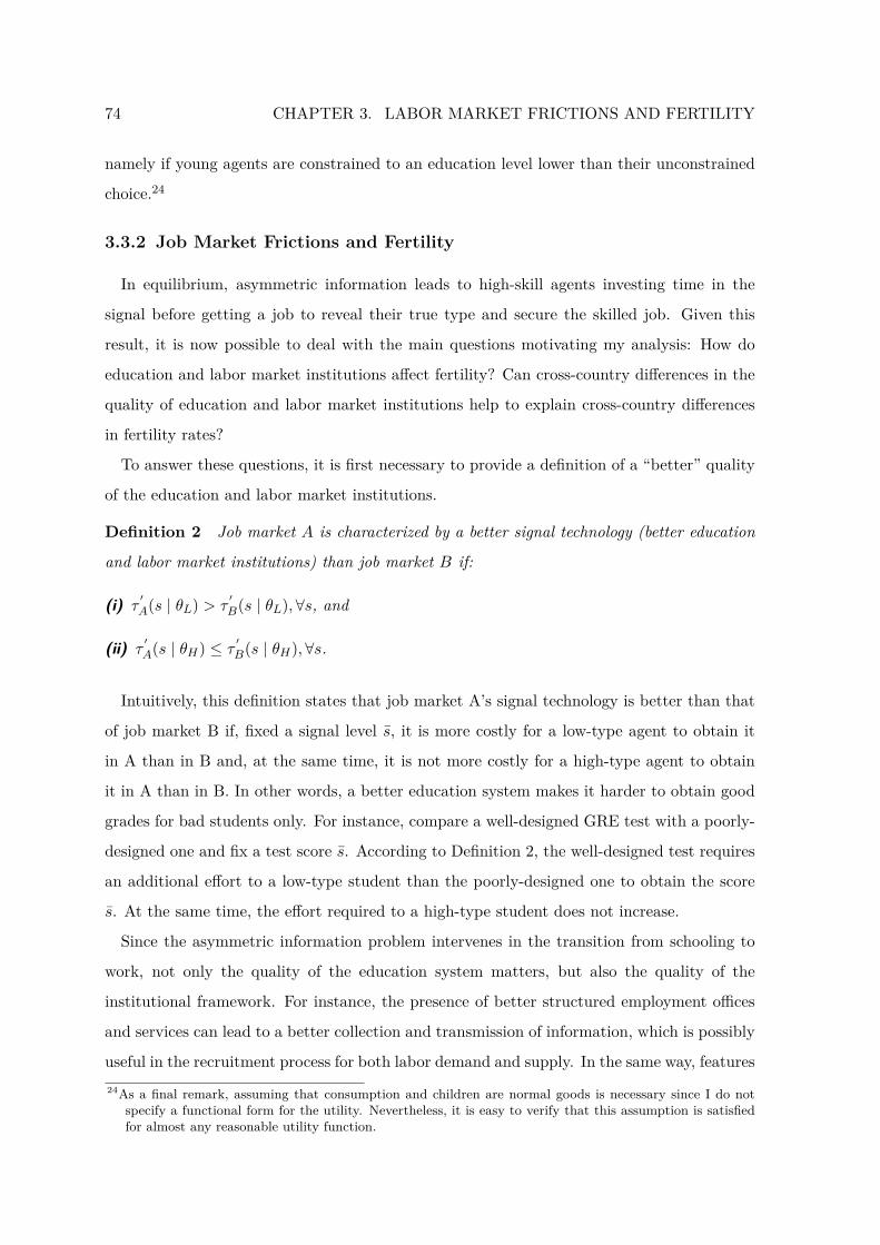
74 CHAPTER 3. LABOR MARKET FRICTIONS AND FERTILITY
namely if young agents are constrained to an education level lower than their unconstrained
choice.24
3.3.2 Job Market Frictions and Fertility
In equilibrium, asymmetric information leads to high-skill agents investing time in the
signal before getting a job to reveal their true type and secure the skilled job. Given this
result, it is now possible to deal with the main questions motivating my analysis: How do
education and labor market institutions affect fertility? Can cross-country differences in the
quality of education and labor market institutions help to explain cross-country differences
in fertility rates?
To answer these questions, it is first necessary to provide a definition of a “better” quality
of the education and labor market institutions.
Definition 2 Job market A is characterized by a better signal technology (better education
and labor market institutions) than job market B if:
(i) τ′A(s | θL) > τ
′B(s | θL),∀s, and
(ii) τ′A(s | θH) ≤ τ ′B(s | θH),∀s.
Intuitively, this definition states that job market A’s signal technology is better than that
of job market B if, fixed a signal level s, it is more costly for a low-type agent to obtain it
in A than in B and, at the same time, it is not more costly for a high-type agent to obtain
it in A than in B. In other words, a better education system makes it harder to obtain good
grades for bad students only. For instance, compare a well-designed GRE test with a poorly-
designed one and fix a test score s. According to Definition 2, the well-designed test requires
an additional effort to a low-type student than the poorly-designed one to obtain the score
s. At the same time, the effort required to a high-type student does not increase.
Since the asymmetric information problem intervenes in the transition from schooling to
work, not only the quality of the education system matters, but also the quality of the
institutional framework. For instance, the presence of better structured employment offices
and services can lead to a better collection and transmission of information, which is possibly
useful in the recruitment process for both labor demand and supply. In the same way, features24As a final remark, assuming that consumption and children are normal goods is necessary since I do not
specify a functional form for the utility. Nevertheless, it is easy to verify that this assumption is satisfiedfor almost any reasonable utility function.

75
of an organized stock exchange such as price transparency, a central method of clearing trades,
a stable regulatory framework and liquidity improve the connection between the demand and
supply of stocks and bonds. Therefore, a better signal technology can also be interpreted as
a higher quality of labor market institutions.25
As the left panel of Figure 3.4 shows, when the signal technology is better, the low-type
agents’ indifference curves on the Cartesian space S × W are steeper, while those of the
high-type agents are not. This implies that the incentive for low-type agents to invest in
the signal to simulate being of high type are lower, given that the cost of doing so is higher.
Consequently, in equilibrium it is easier for high-type agents to obtain a signal level sufficient
to reveal their true type.
Proposition 2 below characterizes the main result of the paper, namely the effect that a
better signal technology has on the equilibrium fertility rate.
Proposition 2 If job market A is characterized by a better signal technology than job market
B, then the unique equilibrium surviving refinements in A is characterized by:
(i) a lower signal level for the θH workers: s∗A(θH) = sA < sB = s∗B(θH);
(ii) a lower signal cost for the θH workers: τA(sA | θH) < τB(sB | θH);
(iii) a higher youth employment: 1− ατ(sA | θH) > 1− ατ(sB | θH); and
(iv) a higher fertility rate.
Proof See the appendix.
3.3.2.1 Signal Technology and Fertility: Discussion
When the signal technology is better, the signal level that allows high-type workers to
reveal their true type is lower (left panel of Figure 3.4). This result is due to the smaller
incentive for low-skill workers to mimic the education choice of high-skill workers, owing to
the higher cost of doing so. As the time that high-skill workers need to invest in signal
is lower, they can start working earlier and their income increases. Given that child-rearing
costs are more affordable to high-skill workers, they choose to have more children (right panel
of Figure 3.4).
25Concerning labor regulation more specifically, Proposition 4 below characterizes the effect on fertility of aregulation that limits job contract renegotiation or does not.

76 CHAPTER 3. LABOR MARKET FRICTIONS AND FERTILITY
Figure 3.4: Better signal technology and its effect on fertility
A second, forward-looking effect on fertility is also realized if in country B, the optimal
transfer that low-income parents give to their high-type children is exactly as large as needed
to allow them to choose s∗ (θH). In this case, these parents are transferring to their children
more resources than they would have done in a frictionless world, with perfectly observable
agents skills. While they do so to allow their children to gain a better wage in the next
period, such a large cost has the effect of constraining the parents’ fertility choice today.
By contrast, in country A, where the signal technology is better, the education investment
needed to high-type workers to separate themselves from the low-type ones and gain the
high wage is lower. Accordingly, the resources needed to finance the consumption of children
investing in education are lower; thus, the optimal parental transfer can be lower in A than
in B, as Figure 3.5 shows. What does this imply for fertility? As children will start to work
earlier and will rely less on their parents to consume in the next period, today parents face
a lower overall child-rearing cost and thus they have more resources available to devote to
consumption and fertility. Therefore, a second price effect of signal technology leads to an
even higher total fertility rate in country A.
To conclude this brief discussion concerning the model behavior, recall the crucial moti-
vating question stated above: Can cross-country differences in the quality of education and
labor market institutions help to explain cross-country differences in fertility? The answer
provided by the model mechanisms is affirmative. Differences in the quality of education
and labor market institutions matter for the fertility choice, as they affect: (i) the time that
young workers need to find a job, the youth labor force participation and ultimately the
young workers’ income; and (ii) the expenses that parents have to sustain to finance the
77
Figure 3.5: Optimal transfer and better signal technology
consumption of their children investing in education.
Recall the opportunity cost of parental time channel underlined by the standard fertility
literature. According to this theoretical mechanism, the fact that the US fertility rate is
higher than e.g. the Italian one is somewhat puzzling, given that both the higher US female
labor force participation and the higher per capita income render the opportunity cost of
parental time higher. By contrast, the channels highlighted by this model underline two
reasons discouraging fertility more in Italy compared with the US: first, young people start
to work later and youth employment is lower, whereby child-rearing costs are less affordable
to young parents; and second, Italian parents can anticipate that - given the labor market
conditions - they will need to sustain their children’s consumption for a longer period of
time, whereby they actually face higher child-rearing costs. In the light of these channels,
it is unsurprising that Italy displays a lower fertility rate than US: even if the higher US
per capita income makes the parental opportunity cost of time higher, those two effects may
outweigh this last one.
3.3.3 Labor Market Regulation
The nature of the asymmetric information friction considered here makes it interesting to
analyze how the labor regulation provides incentives for the workers’ and firms’ decisions.
Therefore, this section analyzes the impact of labor regulation on fertility as a possible addi-
tional source to explain the observed cross-country differences in fertility.
A common and empirically relevant hypothesis in the literature is that employers learn

78 CHAPTER 3. LABOR MARKET FRICTIONS AND FERTILITY
about the productivity of workers over the working relationship.26 I follow this hypothesis
in this model extension, assuming that - at the completion of the first working period -27
employers have acquired sufficient additional information to infer the true worker’s type. In
other words, at the beginning of the second working period, asymmetric information vanishes
and the worker’s type is observable to the employer. In this case, the employer or employee
might have interest in renegotiating the job contract. However, labor regulation often imposes
limits to a free renegotiation of job contracts, particularly if it can worsen workers’ conditions.
There are several reasons why governments intervene in the labor market. For instance,
in a completely free labor market, employers can find it profitable to discriminate against
disadvantaged groups, fire workers who subsequently need to be supported by the state, force
employees to work more than they wish or underpay them under the threat of dismissal,
and so on. In response to the perceived unfairness and inefficiency of a completely free
market employment relationship, almost every state intervenes in this relationship to protect
the workers. The regulation of labor markets aimed at protecting workers takes different
forms. For example, governments regulate employment relationships by restricting the range
of feasible contracts and limiting their free renegotiation.28 Accordingly, the labor regulation
imposes stronger limits to a free renegotiation of the employment contracts in some countries
than others.
In the model, the two following stylized cases are considered as proxies for the rigidity of
the labor regulation: (i) free renegotiation of the job contracts is allowed; and (ii) any change
in the job contract worsening workers’ conditions is not allowed. In other words, the wage
and the position offered by the firm at the beginning of the employment can be only improved
in this second scenario.
Whether the first or the second of these two regimes is implemented crucially affects youth
employment and fertility, as the following proposition shows.
Proposition 3 Assume that - at the beginning of the third period of life - the agents’
types become observable. Then allowing for free job contracts renegotiation leads to a Pareto
improvement and increases the equilibrium employment and fertility rates.
Proof See the appendix.
26See, e.g. Farber and Gibbons (1996), and Altonji and Pierret (2001).
27Recall that in the model, a time period corresponds to a third of the life of an agent.28For a more detailed discussion about government intervention in the labor market, see for instance Botero
et al. (2004)

79
The mechanism at work here can be summarized as follows. If the employer is free to
change the contract, once the worker’s type is revealed he/she will receive a wage equal to
his/her true marginal productivity, independent of the signal investment made. On the other
side, if worsening contract renegotiation is not allowed, the worker will keep the same wage
as in the previous period, independent of his/her true type. Therefore, if the renegotiation is
allowed, low-type workers have a weaker incentive to invest in signal to simulate being of high
type. By mimicking the education choice of high-skill workers, they would receive the high
wage, albeit only in the first period. In the second period, their true ability will be known
and firms will be able to change their contracts, reducing the wage to their actual marginal
product. Lower incentives for low-type workers to invest in education means that it is easier
for high-type workers to reveal their true type to the market; namely, they need to invest less
time in signal and they can start to work earlier. Through the two mechanisms described in
Proposition 2, this result translates into a higher equilibrium fertility rate.
It is interesting to note that the free renegotiation leads to a Pareto-superior equilibrium
with respect to the other case. High-type workers are better off, while low-type workers do
not lose anything, since in equilibrium they choose not to invest in signal, obtaining the low
wage regardless.
Therefore, in the simple model considered, less rigidity in the labor market successfully
reduces the negative impact of asymmetric information, consequently increasing employment
and fertility. This result suggests that - despite aiming at protecting workers - the labor
regulation can reduce workers’ welfare if producing excessive rigidity, also with negative
consequences for fertility.
3.3.4 Time Cost of Children
In the last part of this section, I extend the model to analyze the robustness of its predictions
to the introduction of a time cost of children. Introducing this feature might have crucial
consequences, as it becomes no longer obvious that a higher parental income implies a higher
fertility: the time cost of child-rearing introduces a negative substitution effect that might
outweigh the described positive effects of a better signal technology on fertility. Indeed, in line
with the channel highlighted by the standard fertility literature, an increase in income now
makes fertility more expensive, given that the opportunity cost of parental time increases.
Therefore, this extension allows considering all these mechanisms as a whole to verify their

80 CHAPTER 3. LABOR MARKET FRICTIONS AND FERTILITY
net effect on fertility.
As the time cost of child-rearing makes the problem of the job market equilibria existence
hardly tractable, I introduce some simplifying assumptions. First, I restrict the analysis to
the case of logarithmic preferences. Second, I assume that parents no longer decide how much
to transfer to their children; rather, financing the consumption of their children investing in
education is a cost that appears in their budget constraint. A further simplification leading
to closed form solutions is that parents do not discount the future utility of their children,
enjoying instead children as a consumption good.29
Therefore, the maximization problem of a young adult of type θ is now given by:
maxc1,c2,n,s
U(c1, c2, n) = (1− λ) ln c1 + λ lnn+ β [(1− λ) ln c2 + λ lnn]
s.t. c1 + c21 + r
+ (ρ+ Ψθ)n ≤(
1− τ(s | θ)− φn+ 11 + r
)w,
where λ measures how much parents enjoy having children compared to their own consump-
tion, φ is the time cost of rearing a child and
Ψθ = ϕαθτ(s | θH) + (1− αθ)τ(s | θL)
1 + r
is the discounted per child consumption cost that parents sustain while their children are
investing time in education rather than working. Ψθ is function of the parent’s type, as I
assume now that the share of high-type children possibly depends on the parent’s type, with
a positive correlation between parental and children’s skill.30
Proposition 4 In the problem described:
1. The job market separating equilibrium characterized in Proposition 1 still exists and is
unique.
2. The results in Proposition 2 still apply, namely a better signal technology produces higher
equilibrium employment and fertility rates.
3. If ΨH−ΨLρ+ΨL ≥
θH−θLθL
, the correlation between income and fertility within the economy is
negative.
Proof See the appendix.29This alternative formulation is commonly used in the fertility literature. The absence of the transfer choice
makes it less costly to forgo dynastic utility.30Note that this additional assumption only matters for the 3rd point of Proposition 4.

81
With the introduction of a time cost of child-rearing and a positive correlation between
the child’s and the parent’s types, it is now possible that - within-country - fertility is nega-
tively correlated with income, in line with the empirical evidence that the standard fertility
literature aims at matching.31 However, despite the introduction of the opportunity cost
of parental time mechanism, a better signal technology still leads to a higher equilibrium
fertility rate, as high-type young adults have more time available and optimally decide to in-
crease fertility. Moreover, an improvement in signal technology reduces the expenditure that
parents have to sustain for the future consumption of their children. Consequently, fertility
increases among both parent types.
This result shows that the two mechanisms highlighted in this work are robust to the
introduction of the standard fertility literature main mechanism in the model. With this
extension, the model predictions are possibly consistent with both (i) the negative within-
country relationship between income and fertility and (ii) the cross-country relationship of
fertility vs. employment, income, as well as other labor market indicators analyzed below in
Section 4.
3.4 Model Predictions vs. Data
In this section, I compare the model predictions with European data. I do not consider
all the OECD countries because some of the indicators used here - namely the vertical job
mismatch estimates provided by the Cedefop and the youth financial dependence on parents
estimates provided by Billari and Tabellini (2010) - only include European countries in the
sample. As summarized for convenience in Figure 3.6, the model predicts that countries in
which the signal technology is better will be characterized by: (i) a shorter joblessness time
among young workers; (ii) higher youth employment rates; (iii) a lower financial dependence
of children on parents; and (iv) higher fertility rates, thanks to the young workers’ higher
income and the lower child-rearing cost. These predictions are possibly consistent with a
negative within-country relationship between income and fertility, as an economy will display
- under some conditions - higher fertility for low-income parents compared with high-income
parents. However, different from the standard fertility literature, the model proposed in this
paper is also consistent with the cross-country evidence briefly discussed in the introduction31The need for special assumptions to obtain a negative correlation between income and fertility is common
in the fertility literature. For a detailed discussion on this issue see e.g. Jones, Schoonbroodt and Tertilit(2010).

82 CHAPTER 3. LABOR MARKET FRICTIONS AND FERTILITY
Figure 3.6: Summary of the model results
and presented here.
In the data, it is possible to find quite direct proxies for the model variables listed above
from point (i) to (iv). The fertility rate, the youth employment rate, the youth joblessness
time and the tightness of the young workers’ constraint finda direct coincidence in the data
with the respective OECD estimates of the total fertility rates, the OECD estimates of the
youth employment rates, the number of months needed to find a first job after leaving school
estimated by Quintini and Manfredi (2009),32 and the youth financial dependence estimated
by Billari and Tabellini (2010).33
Table 3.1 shows the correlation coefficients and their significance levels between total fertil-
ity rates and the cross-country levels of the estimates listed above.34 As the model predicts,
data show that developed countries tend to have higher fertility rates when they are char-
acterized by: (i) fewer months needed to find a job after leaving school; (ii) higher youth
employment rates; and (iii) a lower share of young people dependent on their parents or
partner.
However, the relationships reported above do not directly address the main feature of the
model, namely the impact of the signal technology on the labor market and consequently on
fertility. Therefore, a crucial step of this analysis involves identifying an indicator in the data
32The calculations are based upon the National Longitudinal Surveys of Youth 1997 and the European Com-munity Household Survey (1994-2001).
33The estimates are based upon Billari (2004), using Eurobarometer data for 1997 and 2001, as well as theGallup Organization (2007) for 2007.
34Cross-country plots of all the relationships listed in Table 3.1 are shown in Appendix D.

83
measuring cross-country differences in the signal technology.
Recall that the signal technology can be mainly interpreted as the quality of the educa-
tion system, particularly in signaling workers’ abilities to the job market, while the quality
of the institutional framework also matters. For instance, the presence of better structured
employment offices and services can lead to a better collection and transmission of infor-
mation, which is possibly crucial in the recruitment process. Therefore, the goal involves
identifying cross-country estimates capable of providing good proxies for the quality of both
the education system and the institutional framework, which can facilitate the information
transmission between the supply of labor and its demand. Recall also that a worse signal
technology in the model leads high-type workers to a larger over-investment in education, or
over-qualification, to reveal their true skill to their potential employers.
Using the European Union Labour Force Survey (EU-LFS), the European Centre for the
Development of Vocational Training (Cedefop) provides cross-country estimates of the in-
cidence of vertical job mismatch, which I use as main proxy for the quality of the signal
technology. The incidence of vertical job mismatch measures the average share in the labor
force of over-qualified workers as a percentage of the total workers. Over-qualified workers
are those whose highest level of qualification attained is greater than the qualification re-
quirement of their occupation. The modal qualification in each occupational group is used to
measure qualification requirements. I use cross-country negative variations in this indicator
as a proxy for the model cross-country positive variations in signal technology. Therefore, the
lower the share of over-qualified workers, the better the signal technology is, and vice versa.
Why does this indicator provide a good proxy for the quality of signal technology? Con-
sider the following example. If Portugal displays a higher value than Sweden in the Cedefop
measure of vertical job mismatch, it means that - on average - Portuguese workers invest
more in obtaining qualifications than their Swedish colleagues before starting to perform the
same job. Unless Portuguese workers perform better in the job or enjoy obtaining a qualifi-
cation more, this higher value should signal a poorer quality of the Portuguese “qualification
technology” compared with the Swedish one.
The second proxy that I use is the ratio between a country’s total domestic expenditure on
education and its GDP. This should provide a measure of the importance of education in that
country. Positive cross-country variations in the total expenditure on education in relation to
GDP proxy for positive cross-country variations in the quality of education. In other words,
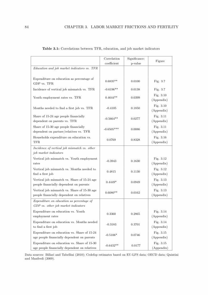
84 CHAPTER 3. LABOR MARKET FRICTIONS AND FERTILITY
Table 3.1: Correlations between TFR, education, and job market indicators
Correlationcoefficient
Significance:p-value
Figure
Education and job market indicators vs. TFR
Expenditure on education as percentage ofGDP vs. TFR
0.6835** 0.0100 Fig. 3.7
Incidence of vertical job mismatch vs. TFR -0.6196** 0.0138 Fig. 3.7
Youth employment rates vs. TFR 0.4644** 0.0399Fig. 3.10
(Appendix)
Months needed to find a first job vs. TFR -0.4105 0.1850Fig. 3.10
(Appendix)
Share of 15-24 age people financiallydependent on parents vs. TFR
-0.5664** 0.0277Fig. 3.11
(Appendix)
Share of 15-30 age people financiallydependent on partner/relatives vs. TFR
-0.6505*** 0.0086Fig. 3.11
(Appendix)
Households expenditure on education vs.TFR
0.0769 0.8328Fig. 3.16
(Appendix)
Incidence of vertical job mismatch vs. otherjob market indicators
Vertical job mismatch vs. Youth employmentrates
-0.3943 0.1630Fig. 3.12
(Appendix)
Vertical job mismatch vs. Months needed tofind a first job
0.4815 0.1130Fig. 3.12
(Appendix)
Vertical job mismatch vs. Share of 15-24 agepeople financially dependent on parents
0.4449* 0.0949Fig. 3.13
(Appendix)
Vertical job mismatch vs. Share of 15-30 agepeople financially dependent on relatives
0.6080** 0.0162Fig. 3.13
(Appendix)
Expenditure on education as percentage ofGDP vs. other job market indicators
Expenditure on education vs. Youthemployment rates
0.3360 0.2865Fig. 3.14
(Appendix)
Expenditure on education vs. Months neededto find a first job
-0.3183 0.3701Fig. 3.14
(Appendix)
Expenditure on education vs. Share of 15-24age people financially dependent on parents
-0.5106* 0.0746Fig. 3.15
(Appendix)
Expenditure on education vs. Share of 15-30age people financially dependent on relatives
-0.6432** 0.0177Fig. 3.15
(Appendix)
Data sources: Billari and Tabellini (2010); Cedefop estimates based on EU-LFS data; OECD data; Quintiniand Manfredi (2009).
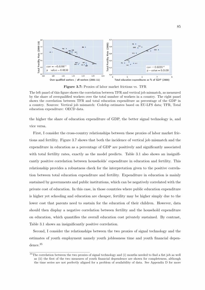
85
Figure 3.7: Proxies of labor market frictions vs. TFRThe left panel of this figure shows the correlation between TFR and vertical job mismatch, as measuredby the share of overqualified workers over the total number of workers in a country. The right panelshows the correlation between TFR and total education expenditure as percentage of the GDP ina country. Sources: Vertical job mismatch: Cedefop estimates based on EU-LFS data; TFR, Totaleducation expenditure: OECD data.
the higher the share of education expenditure of GDP, the better signal technology is, and
vice versa.
First, I consider the cross-country relationships between these proxies of labor market fric-
tions and fertility. Figure 3.7 shows that both the incidence of vertical job mismatch and the
expenditure in education as a percentage of GDP are positively and significantly associated
with total fertility rates, exactly as the model predicts. Table 3.1 also shows an insignifi-
cantly positive correlation between households’ expenditure in education and fertility. This
relationship provides a robustness check for the interpretation given to the positive correla-
tion between total education expenditure and fertility. Expenditure in education is mainly
sustained by governments and public institutions, which can be negatively correlated with the
private cost of education. In this case, in those countries where public education expenditure
is higher yet schooling and education are cheaper, fertility may be higher simply due to the
lower cost that parents need to sustain for the education of their children. However, data
should then display a negative correlation between fertility and the household expenditure
on education, which quantifies the overall education cost privately sustained. By contrast,
Table 3.1 shows an insignificantly positive correlation.
Second, I consider the relationships between the two proxies of signal technology and the
estimates of youth employment namely youth joblessness time and youth financial depen-
dence.35
35The correlation between the two proxies of signal technology and (i) months needed to find a fist job as wellas (ii) the first of the two measures of youth financial dependence are shown for completeness, althoughthe time series are not perfectly aligned for a problem of availability of data. See Appendix D for more

86 CHAPTER 3. LABOR MARKET FRICTIONS AND FERTILITY
Table 1 shows that the incidence of vertical job mismatch is negatively associated with
youth employment, while it displays positive correlations both with the number of months
needed to find a first job after leaving school and the share of young people financially de-
pendent on their parents or partner. The model mechanisms are very consistent with this
evidence. According to Proposition 2, a worse signal technology implies a higher work-
ers’ over-qualification, lower youth employment rates, a longer youth joblessness time and a
stronger youth financial dependence on parents. These effects imply that child-rearing costs
are less affordable to young workers and hence fertility rates are lower.
The model also stresses the role of a second forward-looking channel, according to which
a worse signal technology further reduces fertility by increasing future children expenditure.
Note the positive relationship between vertical job mismatch and the share of young people
financially dependent on their parents, as well as the negative relationship between the latter
measure and fertility reported in Table 1 and Figure 3.11. Those countries whose labor
market is characterized by a stronger incidence of vertical job mismatch are also those where
children rely on their parents’ income for a longer period of time, as well as displaying lower
fertility rates. This evidence is very consistent with the second theoretical channel that the
model highlights.
Table 1 also lists the correlations obtained by using the second proxy, namely total ex-
penditure on education as a percentage of GDP. Again, the cross-country correlations have
the predicted signs, whereby higher total expenditure on education is associated with a lower
numbers of months needed to find a first job, a smaller incidence of children’s financial de-
pendence on their parents and higher youth employment rates.
While a comprehensive empirical analysis of the theoretical issues studied in the previous
sections is beyond the scope of this paper, in light of the empirical evidence reported in this
section, it is possible to conclude that the model predictions display a good qualitative fit
of the data, given that all the cross-countries relationships considered display the predicted
signs.
3.5 Conclusion
The paper presents a theory according to which labor market frictions produced by asym-
metric information depress fertility.
details.

87
Better education and labor market institutions - conceived in the model as better “signal
technology” - reduce the severity of the friction incidence by lowering low-skill workers’ incen-
tive to undertake the path leading to high educational attainments. Consequently, high-skill
workers find a first job more easily and quickly, and the labor market allocation is more
efficient.
The positive effect on fertility is twofold: first, child-rearing costs are more affordable to
young parents, as they start to work earlier and their income is higher; and second, parents
need to sustain their children’s consumption for a shorter period of time, as children will find
a job earlier and hence total child-rearing costs are lower. These two effects lead to the result
that those economies whose education and labor market institutions are better display higher
fertility rates.
By contrast, rigidities produced by an overly-restrictive labor market regulation can have a
similar effect of a worse signal technology by exacerbating the negative impact of asymmetric
information. Low-skill workers have a stronger incentive to mimic the education choice of
high-skill workers. Hence, high-skill workers need to invest more in education to reveal their
true skill to the market. This makes child-rearing costs less affordable and leads to lower
fertility rates.
This mechanism is robust to the introduction of a time cost of child-rearing. The positive
effect on fertility of a better signal technology - with the following increase in the time
available to child-rearing - outweighs the negative effect of an increase in the opportunity
cost of parental time due to a higher income.
This last result implies that the theoretical mechanisms presented - differently to those
proposed by the standard fertility literature - are possibly consistent with the developed
countries evidence in terms of both: (i) the negative within-country relationship between
income and fertility; and (ii) the positive cross-country relationship between fertility and
(both female and overall) employment rates.
Indeed, although a quantification of the impact on fertility of the channels highlighted in
this paper is left to future research, the model displays a good qualitative fit of the data. In
particular, in line with the model predictions, we observe negative cross-country relationships
between fertility rates and several indicators of the incidence of the frictions on labor markets.

88 CHAPTER 3. LABOR MARKET FRICTIONS AND FERTILITY
3.6 Appendix A: Definition of the Refinement H
Definition A.1 (adapted from MWG 13.AA.3) Define W∗(Θ, s) as the set of all
possible equilibrium response w∗(Θ, s), and V (s, w, θ) as the indirect utility function of an
agent of type θ. A PBE satisfies the refinement H if: for all education levels s ∈ S, the
belief function µ(θ | s) assumes values strictly greater than 0 only if, for type θ there is no
equilibrium action s′ such that:
min
w′ ∈W∗(Θ, s′)V (s′, w′, θ) >
max
w ∈W∗(Θ, s)V (s, w, θ).
Intuitively, this refinement imposes that the belief function µ(θ | s) assumes a strictly
positive value only if there is no equilibrium action s′ for a worker of type θ that - even in the
worst possible equilibrium outcome - gives him/her a higher wage than playing s. Otherwise,
a worker of type θ would always prefer to play s′ rather than s, since it ensures a higher
equilibrium payoff. In other words, s is equilibrium dominated for any worker of type θ. The
firms knows this and consequently adjust their belief function by attaching zero probability
to the event that the signal observed s can be a the choice made by a worker of type θ:
µ(θ | s) = 0.

89
3.7 Appendix B: Proofs
3.7.1 Lemma 1 and Proof
This lemma proves that although the signaling game is embedded into an OLG model where
households have many decision variables, the standard assumptions of signaling games remain
sufficient to guarantee the existence of equilibria, and particularly the least cost equilibrium.
In the standard two-type signaling game as described in MWG 13.C, the worker’s utility
function takes the simplified form u(w, s, θ) = w − t(s | θ). The two conditions: (i) t′(s |
θ) > 0, t′′(s | θ) > 0, and (ii) t′(s | θL) > t′(s | θH), ∀s, are sufficient for the existence of
pooling and separating equilibria, because they guarantee that the agents’ indifference curves
(i) have a positive slope and convexity and (ii) satisfy single crossing. Similarly, I prove that
Assumption 1 is sufficient to generate similar agents’ behaviors in the extended framework
analyzed here.
Lemma 1 Define S ×W as the R2++Cartesian plane including all the pairs of wage w ∈
W ⊆ R+ and signal s ∈ S ⊆ R+, and consider the indifference curves on S×W of a type θ
household, whose maximization problem is described in Section 2.1.
Assume that the constraint (3.3) in the young adults’ optimization problem is not binding
or is binding at the unconstrained optimum s∗(θ). Under Assumption 1, the indifference
curves on S×W of a household of any type θ satisfy the following conditions:
1. Positive slope and convexity, namely: dwds > 0, d2w
ds2 > 0.
2. The low-type’s indifference curves and the high-type’s ones satisfying single crossing,
namely: dwds |θ=θL>
dwds |θ=θH , ∀s.
Proof From the budget constraint of a type θ household’s max problem described in Section
2.1, define the net income B (w, s | θ) ≡ (1− τ(s | θ) + 11+r )w + T−1
θ .
Assume that the instantaneous utility function u(·) in any type θ household’s problem
represents rational, monotonic, strictly convex and continuous preferences. Subsequently,
the necessary and sufficient conditions for a maximum of the household’s problem - with w
and s parameters - define the indirect utility function V (B (w, s | θ)), which is continuous
and increasing in B.
An indifference curve of a type θ household on the Cartesian space S ×W is defined as
the set of points such that V (B (w, s | θ)) = constant.

90 CHAPTER 3. LABOR MARKET FRICTIONS AND FERTILITY
Totally differentiating the above relationship with respect to s, we obtain:
dV (B (w, s | θ))ds
= ∂V (B (w, s | θ))∂B
∂B (w, s | θ)∂w
dw
ds+ ∂V (B (w, s | θ))
∂B
∂B (w, s | θ)∂s
= 0
⇔ dw
ds= −
∂V (B(w,s|θ))∂B
∂B(w,s|θ)∂s
∂V (B(w,s|θ))∂B
∂B(w,s|θ)∂w
= τ′(s | θ)w
1− τ(s | θ) + 11+r
.
By Assumption 1, τ ′(s | θ) > 0 and τ(s | θ) < 1, then:
τ′(s | θ)w
1− τ(s | θ) + 11+r
> 0.
Moreover, since by Assumption 1 τ ′′(s | θ) > 0,
d2w
ds2 =w[τ ′′(s | θ)
(1− τ(s | θ) + 1
1+r
)+ (τ ′(s | θ))2
](1− τ(s | θ) + 1
1+r
)2 > 0.
Therefore, the above-stated condition (i) is satisfied.
Moreover:
dw
ds|θ=θL= τ ′(s | θL)w
1− τ(s | θL) + 11+r
>τ ′(s | θH)w
1− τ(s | θH) + 11+r
= dw
ds|θ=θH , ∀s,
since, by Assumption 1, τ ′(s | θL) > τ ′(s | θH) and τ(s | θL) > τ(s | θH), ∀s. Therefore, the
above-stated condition (ii) (single crossing) is also satisfied. It is possible to conclude that,
under Assumption 1, the job market described in Section 2.2 exhibits pooling and separating
equilibria. �
3.7.2 Proof of Proposition 1
2 (i) (Continuum of separating equilibria) By using the results of Lemma 1, the proof
follows the same steps as in the standard two-type signaling game. Therefore, see MWG
13.C, p. 453 ff. However, as the signal is assumed to cost time rather than money, one can
argue that a time inconsistency problem may affect the separating equilibria of the game.36In
36The critical argument develops as follows. Suppose that the least cost separating is a PBE of a game likethe one described, albeit played over continuous time. Given the time cost assumption, s = 0 correspondsto start working immediately. In the equilibrium candidate considered, all and only the low-type workerschoose s∗(θL) = 0. However, a while after that the low wage contracts are signed, firms know that allthe remaining workers are of high type and consequently adjust their belief function µ(s). The only belieffunction consistent with Bayes’ rule will be µ (θH | s > 0) = 1. Therefore, no longer for s only, but even

91
fact, time is discrete in the OLG model considered here, which implies that all the decision
variables are set at the beginning of the period, whereby no time inconsistency problem can
ever arise. �
2 (ii) (One pooling equilibrium) In the following, I assume that the job contracts only
specify the wage, whereby firms are free to employ the workers how they like. If the contract
has to specify both the wage and the job position, the construction of the proof is slightly
different yet it leads to the same result. In a pooling, firms do not distinguish workers’
type; thus, they have to randomly assign new workers to skilled or unskilled labor. Given
the technology assumed, the expected production of a firm randomly assigning 0 ≤ p ≤ 1
workers to LU and (1− p) to LS is given by:
E [Y ] = pθL + (1− p)θH[α+ (1− α) γ
θH
].
If γ < θL − α1−α (θH − θL), then E[Y ] is linearly increasing in p. However, a firm can then
increase its expected profits by simply moving workers from LS to LU and paying them the
same wage. Therefore, in equilibrium it must be the case that p∗ = 1, and all the workers
are assigned to the unskilled labor.
Given that all the workers are employed as LU , they all produce θL, regardless of their type.
In equilibrium, the wage cannot be higher than the labor marginal product - otherwise firms
make losses - nor can it be smaller owing to Bertrand competition. Thus, in equilibrium,
it must be that w∗(s) = θL, ∀s. However, then any s > 0 - given the wage schedule - is
dominated for both workers’ type by s = 0, which implies that s∗(θH) = s∗(θL) = 0.
Therefore, there is a unique pooling PBE, in which s∗(θH) = s∗(θL) = 0 and w∗(s) =
θL, ∀s. �
1 (Unique equilibrium surviving requirement) Standard by using the Intuitive crite-
rion, see MWG 13.AA, p. 470 ff. Note that in this case, the use of Assumption 2 is irrelevant,
for level of signal slightly larger than 0, Bertrand competition will imply that the high wage is offered,w∗(s) = θH , ∀s ∈ (0,∞). The high-type workers will consequently switch from s to a level of signal slightlylarger than 0. However, these contracts are also strictly preferred by low-type workers. At the beginning ofthe game, low-type workers will anticipate the way in which firms beliefs will be updated, then s(θL) = 0is no longer a best response. Thus, the least cost separating outcome is no longer a PBE. This argumentwould equivalently apply for any other separating outcome. Note that this game will not suffer from thistime inconsistency problem by assuming that at least one of the following conditions does not apply: (i)the age of any worker and the moment in which he/she possibly started education is perfectly observableto firms; (ii) education is a continuous choice; and (iii) agents and firms have no possibility of commitment.See Noldeke and Van Damme (1990) for a more detailed discussion about this issue, as well as an exampleof a game played over continuous time where the least cost separating equilibrium survives.

92 CHAPTER 3. LABOR MARKET FRICTIONS AND FERTILITY
as the claim will result also assuming the standard 2-type game condition that low-type and
high-type workers produce θL and θH , respectively, regardless how they are employed.
Using the weaker refinement H, first all the separating PBE aside from the least cost one
are ruled out. For the low-type worker ∀s > s is equilibrium dominated, then a firm observing
a signal larger than s must know that the worker is of high type. Subsequently, the belief
function µ(θH | s) = 1, ∀s ≥ s. This implies that w∗(s) = θH , ∀s ≥ s. However, then any
s > s - given the wage schedule - is dominated for a high-type worker by s = s. Therefore,
no separating equilibrium with s∗(θH) > s survives.
Second, the only pooling PBE is also ruled out. Given that the only reasonable belief
function must be µ(θH | s) = 1, ∀s > s, for the high-type worker not to invest in the signal,
s∗(θH) = 0, is strictly dominated by s∗(θH) = s. Therefore, the pooling equilibrium does not
satisfy the belief refinement H. �
3.7.3 Proof of Lemma 2
Consider the problem of a parent of type θ in his third period of life, when the fertility
decision is already taken:
maxc2,{Tθ}
u(c2) + λn1−η (αVH(TH) + (1− α)VL(TL))
s.t. c2 + n (αTH + (1− α)TL) ≤ (1 + r)[(1− τ(s | θ) + 1
1 + r)wθ + T−1
θ − c1 − nρ]
︸ ︷︷ ︸≡ B (net available income)
When parental transfers reduce, a parent can increase his/her own consumption and u(c2),
but his/her children’s future consumption reduces.
For the moment, suppose all children have the same skill. Plug the budget constraint into
the objective function, to obtain the equivalent problem:
maxT
U(T ) = u (B − nT ) + λn1−ηV (T ).
The parent’s utility moves with the transfer according to:
∂U(T )∂T
= −nu′(c2) + λn1−ηV ′(T ).

93
Consider the parent’s utility U(T ) at the boundaries. At the right boundary, T = Bn =
T , the parent transfers all his wealth to his/her children, and his/her own consumption isnull. For any instantaneous utility function u(·) satisfying the Inada conditions, in the leftneighborhood of T the parent’s utility is strictly decreasing in the transfer, and the optimummust be for T ∗ < T , given that:
∂U(T )∂T
|c2=0= −nu′(c2) + λn1−ηV ′(T ) |c2=0 < 0 ∀λ <∞, since limc2→0
u′(c2) =∞. (3.4)
T = 0 cannot be excluded with a similar argument. At that point the children’s utility is
not necessarily null, since they can choose no education and obtain the low wage; therefore,
it is not obvious that U(T ) is increasing in the right neighborhood of T = 0.
Consider interior points. If the instantaneous utility function u(·) is well behaved, U(T )
will be smooth for any T .
Consider now that children are heterogeneous in skill. If TL, TH < ϕτ(s∗ | θH) ⇒ VH =
VL, since both high and low-type children will be unskilled laborers and have the same
consumption path;37 therefore, in equilibrium it must be T ∗H = T ∗L. For TH ≥ ϕτ(s∗ | θH),
the high-skill children will have a higher consumption path, since they will be able to reveal
their type and obtain the high wage.
Thus, U(TH , TL) is smooth everywhere in TL while it has a discontinuity in TH , namely it
has a jump for TH = ϕτ(s∗ | θH): the parent knows that, for levels beyond this threshold, any
of his/her skilled children will be able to get a higher consumption path. For TH > ϕτ(s∗ |
θH), U(TH , TL) is again smooth in both arguments - but with VH > VL - and, given (3.4), at
some point it start to decrease. Therefore, the parent’s utility as function of TH must look
like in Figure 3.3.
In case 1 and 2, the optimal transfer is sufficiently high, T ∗H ≥ ρτ(s∗ | θH). The constraint
(3.3) in the young adults problem is not binding, or is binding at the unconstrained max for
s, and all the results previously obtained are unchanged. On the other hand, in case 3 and
37If parents’ income is observable, in the separating equilibrium firms will know that, among workers choosings = 0, a share of low income parents’ children is of high type. However, for γ sufficiently small, the sameargument as in the proof of Proposition 1 applies: firms prefer to employ any worker who chooses s = 0as unskilled laborer rather than randomizing. Then, the unique equilibrium is the least cost separatingdepicted in Figure 3.8 below. In the standard signaling framework (that is: without the modificationsproduced by Assumption 1), the outcome surviving the Intuitive Criterion would be slightly different, butwithout compromising the argument of this proof. Constrained high-type and low-type agents would stillchoose s = 0, both of them getting as wage their joint expected marginal product. The unconstrainedhigh-type agents would get a wage equal to θH , s would reduce. Notice that the jump in the wage ofconstrained high-type agents as the constraint is no longer binding would still be present. This feature isthe only needed for the argument of this proof.

94 CHAPTER 3. LABOR MARKET FRICTIONS AND FERTILITY
4 the optimal transfer to high-skill children does not allow them to reveal their true type.
To study case 3, let us analyze how the optimal transfer changes with the parent’s available
income B. For the moment, suppose that all children have the same skill. In any interior
solution, the following first order condition must hold:
∂U(T ∗)∂T
= −nu′ (B − nT ∗) + λn1−ηV ′(T ∗) = 0.
Totally differentiating the FOC with respect to B, we obtain:
dT ∗
dB= 1n+ λV ′′(T )
nηu′′(B−nT )
> 0, sinceV ′′ andu′′must have the same sign.
When children are homogeneous in skill, the optimal transfer is increasing in the parent’s
available income. When children are heterogeneous, the parent’s utility has a jump in TH for
a certain level, but the previous property remains valid. Thus, for a low level of the parent’s
available income, it is possible that we are in the case 3 in the figure; as the parent’s income
increases, we move from case 3 to case 2; and finally, as the income increases further, we
move from case 2 to case 1.
Note also that, in an interior maximum, dc∗2dB > 0 as well: totally differentiating the FOC
with respect to B, we obtain dc∗2dB = 1
1+ n1+ηu′′(c2)
λV ′′(B−c2n
) > 0. I use this result below.
I proved that the optimal transfer is increasing in the 3-period available income B, dT ∗dB > 0.
We want that dT∗dw > 0, for which is sufficient to prove that B increases in w. To do so, consider
now a parent’s problem in the previous period, as a young adult - as stated in Section 2.1.
First, note that in any interior optimum: u′(c∗2) = 1β(1+r)u
′(c∗1) ⇒ dc∗2dc∗1
= 1β(1+r)
u′′(c1)u′′(c2) > 0.
This implies that c1 and c2 are both normal or both inferior goods.
If they are both normal, then dc∗2dw > 0. Previously I showed that dc
∗2
dB > 0 as well. Then, as w
increases, c∗2 increases, then B increases as well. Given that dT ∗
dB > 0, it is possible to conclude
that dT∗dw > 0 as well. Therefore, to assume that consumption is normal is sufficient to obtain
dT∗dw > 0.38 Thus we can conclude that, as the parent’s income increases, we move from case
3 to case 2; as the income increases further, we move from case 2 to case 1. Then there
is a threshold wU in the low wage such that, for wU ≥ wU , for any parent’s and children’s
type, the constraint (3.3) in the young adults problem is not binding, or is binding at the
38Note that, by the property that B is increasing in w, if B ≥ B is satisfied for a parent of type θL, than itmust be satisfied for a parent of type θH too.

95
unconstrained optimum s∗(θ).
It is only left to analyze case 4. For the moment, neglect that children are heterogeneous
in skill. By assuming an interior solution for c1, c2, n, it is possible to rearrange the FOC’s
and obtain the following optimality condition:
nη = λ(1− η)V (T )u′(c2) ((1 + r)ρ+ T ) .
Plugging it into (3.3), we obtain the following sufficient condition to have that T ∗ > 0:
1− η(1 + r)ρ <
V ′(T )V (T ) |T=0 .
It trivially follows that this condition is sufficient to obtain T ∗ > 0 also when children are
heterogeneous in skill. The statement in Lemma 2 follows. �
3.7.4 Proof of Proposition 2
1 (i) In the least cost separating equilibrium, si (i ∈ {A,B}) is implicitly defined by:
V
((1 + 1
1 + r
)θH , si | θL
)= V
((1 + 1
1 + r
)θL, 0 | θL
).
This is true if and only if:
(1− τi(si | θL) + 1
1 + r
)θH =
(1 + 1
1 + r
)θL
⇒ 1θH
(1 + 1
1 + r
)(θH − θL) = τi(si | θL)
⇒ τA(sA | θL) = τB(sB | θL).
By Assumption 2: τ ′(s | θL) > 0. By Definition 1: τ ′A(s | θL) > τ′B(s | θL),∀s. Subsequently,
it follows that sA < sB. �
1 (ii) Given that sA < sB, and by Definition 1 τ ′A(s | θH) ≤ τ′B(s | θH),∀s, it follows that
τA(sA | θH) < τB(sB | θH). �
1 (iii) In the model, youth employment equals:
1− (ατ (s∗(θH) | θH) + (1− α)τ (s∗(θL) | θL))

96 CHAPTER 3. LABOR MARKET FRICTIONS AND FERTILITY
In equilibrium: (a) from 1(i), s∗A(θH) = sA, s∗B(θH) = sB, s∗i (θL) = 0; (b) from 1(ii),
τA(sA | θH) < τB(sB | θH).
Then youth employment in A equals 1−ατA(sA | θH), which is larger than youth employ-
ment in B, equal to 1− ατB(sB | θH). �
2 A better signal technology has a twofold positive effect on fertility.
First, among high-type agents, income is higher in A :
(1− τA(sA | θH) + 1
1 + r
)θH >
(1− τB(sB | θH) + 1
1 + r
)θH
From the utility maximization problem, n∗(w, s) = z((
1− τ(s | θ) + 11+r
)w). From Lemma
2, z′(·) > 0. Then n∗A(θH) > n∗B(θH).
Second, if at least for low-type parents T ∗H,B = ϕτB(sB | θH), then T ∗H,A ≤ T ∗H,B, with
T ∗H,A < T ∗H,B unless dV (·)dTH
= 0. Subsequently, in A, at least low-type parents’ budget set
expands, which implies n∗A(θL) > n∗B(θL).
It follows that the aggregate fertility rate is higher in A compared to B. �
3.7.5 Proof of Proposition 3
Assume that old adults’ type at the beginning of any period is revealed and is public
information.
The equilibrium s = s∗(θH) when contract renegotiation is not allowed is implicitly
defined by:
V
((1 + 1
1 + r
)θH , s | θL
)= V
((1 + 1
1 + r
)θL, 0 | θL
)
⇔(
1− τ(s | θL) + 11 + r
)θH =
(1 + 1
1 + r
)θL.
The equilibrium s = s∗(θH) when contract renegotiation is allowed is implicitly defined
by:
V
(θH + θL
1 + r, s | θL
)= V
((1 + 1
1 + r
)θL, 0 | θL
)
⇔ (1− τ(s | θL)) θH + θL1 + r
=(
1 + 11 + r
)θL

97
The two conditions above imply that:
(1− τ(s | θL) + 1
1 + r
)θH = (1− τ(s | θL)) θH + θL
1 + r.
Given that θH1+r >
θL1+r , it follows from the previous conditions that:
(1− τ(s | θL)) θH < (1− τ(s | θL)) θH ⇒ τ(s | θL) > τ(s | θL)⇒ s > s.
By applying Proposition 2, it follows that the aggregate fertility and youth employment
rates increase as s∗(θL) reduces. Therefore, allowing for job contract renegotiation increases
fertility and youth employment. �
3.7.6 Proof of Proposition 4
1. (Existence and uniqueness) Recall the max problem of a young adult of type θ as
described in Section 3.4. Ignore for the moment the choice of s. The problem is equivalent
to maximizing the following Lagrangian:
L = (1− λ) ln c1 + λ lnn+ β [(1− λ) ln c2 + λ lnn]
−µ[c1 + c2
1 + r+ (ρ+ Ψθ)n−
(1− τ(s | θ)− φn+ 1
1 + r
)w
],
which gives the following FOCs:
(I) (1−λ)c1
= µ
(II) β(1−λ)c2
= µ1+r
(III) λ(1+β)n = µ (ρ+ Ψθ + φw)
(IV) budget constraint
Solving the system, we obtain:
c∗1(w, s) = 1− λ1 + β
[(1− τ(s | θ) + 1
1 + r
)w
],
c∗2(w, s) = β(1 + r) (1− λ)1 + β
[(1− τ(s | θ) + 1
1 + r
)w
],
n∗(w, s) =λ(1− τ(s | θ) + 1
1+r
)w
ρ+ Ψθ + φw.

98 CHAPTER 3. LABOR MARKET FRICTIONS AND FERTILITY
Define V (w, s) ≡ U (c∗1(w, s), c∗2(w, s), n∗(w, s)). We have that:
V (w, s) = (1− λ) ln{1− λ
1 + β
[(1− τ(s | θ) + 1
1 + r
)w
]}
+β (1− λ) ln{β(1 + r) (1− λ)
1 + β
[(1− τ(s | θ) + 1
1 + r
)w
]}+λ(1+β) ln
λ(
1− τ(s | θ) + 11+r
)w
ρ+ Ψθ + φw
= (1 + β) ln
{(1− τ(s | θ) + 1
1 + r
)w
}− λ(1 + β) ln {ρ+ Ψθ + φw}
+ TERMS INDEPENDENT OF w AND s.
I follow a similar strategy as in Lemma 1. Sufficient conditions for the existence of the
equilibrium in the standard signaling game are: (i) positive and convex indifference curves on
the Cartesian space S×W: dwds > 0, d2w
ds2 > 0, and (ii) single crossing: dwds |θ=θL>
dwds |θ=θH , ∀s.
By the Implicit Function Theorem, we obtain:
dw
ds= −
∂∂s [V (w, s)]∂∂w [V (w, s)]
=[
wτ ′(s | θ)1− τ(s | θ) + 1
1+r
] [1 + λφw
ρ+ Ψθ + (1− λ)φw
]> 0 for τ ′(s | θ) > 0.
d2w
ds2 = w
[1 + λφw
ρ+ Ψθ + (1− λ)φw
]τ ′′(s | θ)(
1− τ(s | θ) + 11+r
)+ [τ ′(s | θ)]2(
1− τ(s | θ) + 11+r
)2
> 0 for τ ′′(s | θ) > 0.
dw
ds|θ=θL>
dw
ds|θ=θH ⇔
[wτ ′(s | θL)
1− τ(s | θL) + 11+r
] [1 + λφw
ρ+ ΨL + (1− λ)φw
]>
[wτ ′(s | θH)
1− τ(s | θH) + 11+r
] [1 + λφw
ρ+ ΨH + (1− λ)φw
],
which - given ΨL ≤ ΨH - is true if τ ′(s | θL) > τ ′(s | θH) and τ(s | θL) > τ(s | θH).
Again, the standard conditions used in the signaling literature are sufficient for the exis-
tence of the separating equilibria. Proposition 1 applies unchanged, then the unique equilib-
rium surviving the refinement is the least cost separating equilibrium, in which s∗(θL) = 0,
s∗(θH) = s, w∗H = θH , w∗L = θL. �

99
2. (Signal technology and fertility) Recall the optimal fertility choice of a parent of
type θ:
n∗(w, s) =λ(1− τ(s | θ) + 1
1+r
)w
ρ+ Ψθ + φw.
Notice that: (i) dn∗(·)dτ(s|θ) < 0, and (ii) dn∗(·)
dΨθ < 0.
In the unique equilibrium: s∗(θL) = 0, s∗(θH) = s, w∗H = θH , w∗L = θL. Then: τ(s | θH) =
τ(s | θH), τ(s | θL) = 0, Ψθ = ϕαθτ(s|θH)1+r .
As τ(s | θH) reduces as the signal technology increases, (i) implies that, among high-
type agents, an improvement in signal technology increases fertility. As Ψθ reduces as the
signal technology increases, (ii) implies that, for both parents type, an improvement in signal
technology increases fertility. Therefore, it is possible to conclude that Proposition 2 applies.
�
3. (Within-country income vs. fertility) In equilibrium, the optimal fertility of a
high-type and high income parent is lower than the optimal fertility of a low-type and low
income parent if:
n∗(θH) =λ(1− τ(s | θH) + 1
1+r
)θH
ρ+ ΨH + φθH< n∗(θL) =
λ(1 + 1
1+r
)θL
ρ+ ΨL + φθL⇔
[(ρ+ ΨL) θH + φθLθH ](
1− τ(s | θH) + 11 + r
)< [(ρ+ ΨH) θL + φθLθH ]
(1 + 1
1 + r
),
and ΨH−ΨLρ+ΨL ≥
θH−θLθL
is sufficient to have that n∗(θH) < n∗(θL). �

100 CHAPTER 3. LABOR MARKET FRICTIONS AND FERTILITY
3.8 Appendix C: Robustness and Extensions
This appendix considers model extensions, policy analysis and robustness checks of the
paper’s results.
3.8.1 Binding Constraint at the Education Stage
Lemma 2 provides sufficient conditions under which - in equilibrium - parents of any type
transfer sufficient resources to their high-skill children, allowing them to sufficiently invest in
education to reveal their true type to the market. In other words, the previous results are
obtained under the assumption that nowadays only a negligible minority of talented young
people cannot afford schooling and education in the European developed countries. However,
this case was probably not the most realistic one decades ago.
This section considers what happens if a non negligible part of - even talented - young
people are constrained to a suboptimal choice of education. This extension can provide
insights about the change in sign of the correlation between fertility and female labor force
participation, which occurred in the mid-1980s. To simplify the analysis, I consider a two-
period model.
Recall Lemma 2. If wU < wU , low-income parents’ transfer does not allow their children to
invest s in education (Figure 3.3, case 3) and their choice will be constrained to a certain level
s < s. In equilibrium, the constraint does not bind low-type children’s choice, who do not
invest in signal regardless. However, it does bind high-type children’s choice, who would need
to invest s to reveal their type to the market and can only afford an insufficient level s < s. It
is optimal for these agents not to invest in education and to start working as unskilled laborers,
receiving the low wage.39 Similarly as in Proposition 1, the job market equilibrium surviving
the refinement is the least cost separating outcome. However, in this case, only unconstrained
high-type agents will be employed as skilled laborers, while constrained high-type agents will
be employed as unskilled laborers. Figure 3.8 provides a graphical representation of the
equilibrium.
Do the results summarized in Proposition 2 still apply? In particular, does a better signal
technology still imply a higher fertility?
The first channel through which signal technology influences fertility works in the same
39See Appendix B.I.3, in particular footnote #, for more details.
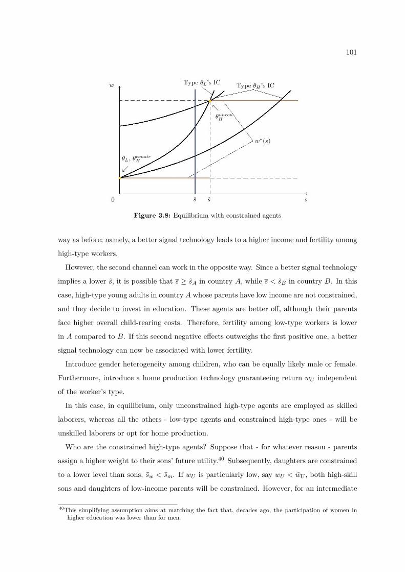
101
Figure 3.8: Equilibrium with constrained agents
way as before; namely, a better signal technology leads to a higher income and fertility among
high-type workers.
However, the second channel can work in the opposite way. Since a better signal technology
implies a lower s, it is possible that s ≥ sA in country A, while s < sB in country B. In this
case, high-type young adults in country A whose parents have low income are not constrained,
and they decide to invest in education. These agents are better off, although their parents
face higher overall child-rearing costs. Therefore, fertility among low-type workers is lower
in A compared to B. If this second negative effects outweighs the first positive one, a better
signal technology can now be associated with lower fertility.
Introduce gender heterogeneity among children, who can be equally likely male or female.
Furthermore, introduce a home production technology guaranteeing return wU independent
of the worker’s type.
In this case, in equilibrium, only unconstrained high-type agents are employed as skilled
laborers, whereas all the others - low-type agents and constrained high-type ones - will be
unskilled laborers or opt for home production.
Who are the constrained high-type agents? Suppose that - for whatever reason - parents
assign a higher weight to their sons’ future utility.40 Subsequently, daughters are constrained
to a lower level than sons, sw < sm. If wU is particularly low, say wU < wU , both high-skill
sons and daughters of low-income parents will be constrained. However, for an intermediate
40This simplifying assumption aims at matching the fact that, decades ago, the participation of women inhigher education was lower than for men.
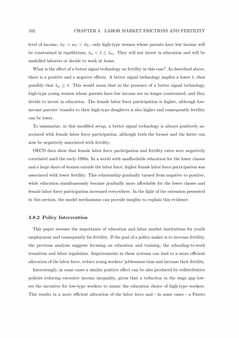
102 CHAPTER 3. LABOR MARKET FRICTIONS AND FERTILITY
level of income, wU < wU < wU , only high-type women whose parents have low income will
be constrained in equilibrium, sw < s ≤ sm. They will not invest in education and will be
unskilled laborers or decide to work at home.
What is the effect of a better signal technology on fertility in this case? As described above,
there is a positive and a negative effects. A better signal technology implies a lower s, then
possibly that sw ≥ s. This would mean that in the presence of a better signal technology,
high-type young women whose parents have low income are no longer constrained, and they
decide to invest in education. The female labor force participation is higher, although low-
income parents’ transfer to their high-type daughters is also higher and consequently fertility
can be lower.
To summarize, in this modified setup, a better signal technology is always positively as-
sociated with female labor force participation, although both the former and the latter can
now be negatively associated with fertility.
OECD data show that female labor force participation and fertility rates were negatively
correlated until the early-1980s. In a world with unaffordable education for the lower classes
and a large share of women outside the labor force, higher female labor force participation was
associated with lower fertility. This relationship gradually turned from negative to positive,
while education simultaneously became gradually more affordable for the lower classes and
female labor force participation increased everywhere. In the light of the extension presented
in this section, the model mechanisms can provide insights to explain this evidence.
3.8.2 Policy Intervention
This paper stresses the importance of education and labor market institutions for youth
employment and consequently for fertility. If the goal of a policy-maker is to increase fertility,
the previous analysis suggests focusing on education and training, the schooling-to-work
transition and labor regulation. Improvements in these systems can lead to a more efficient
allocation of the labor force, reduce young workers’ joblessness time and increase their fertility.
Interestingly, in some cases a similar positive effect can be also produced by redistributive
policies reducing excessive income inequality, given that a reduction in the wage gap low-
ers the incentive for low-type workers to mimic the education choice of high-type workers.
This results in a more efficient allocation of the labor force and - in some cases - a Pareto
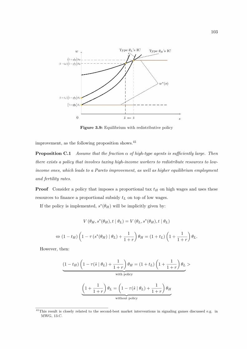
103
Figure 3.9: Equilibrium with redistributive policy
improvement, as the following proposition shows.41
Proposition C.1 Assume that the fraction α of high-type agents is sufficiently large. Then
there exists a policy that involves taxing high-income workers to redistribute resources to low-
income ones, which leads to a Pareto improvement, as well as higher equilibrium employment
and fertility rates.
Proof Consider a policy that imposes a proportional tax tH on high wages and uses these
resources to finance a proportional subsidy tL on top of low wages.
If the policy is implemented, s∗(θH) will be implicitly given by:
V (θH , s∗(θH), t | θL) = V (θL, s∗(θH), t | θL)
⇔ (1− tH)(
1− τ (s∗(θH) | θL) + 11 + r
)θH = (1 + tL)
(1 + 1
1 + r
)θL.
However, then:
(1− tH)(
1− τ(s | θL) + 11 + r
)θH = (1 + tL)
(1 + 1
1 + r
)θL︸ ︷︷ ︸
with policy
>
(1 + 1
1 + r
)θL =
(1− τ(s | θL) + 1
1 + r
)θH︸ ︷︷ ︸
without policy
41This result is closely related to the second-best market interventions in signaling games discussed e.g. inMWG, 13.C.

104 CHAPTER 3. LABOR MARKET FRICTIONS AND FERTILITY
⇒(
1− τ(s | θL) + 11 + r
)>
(1− τ(s | θL) + 1
1 + r
)⇒ τ(s | θL) < τ(s | θL)⇒ s < s.
Subsequently, if the policy is implemented, the equilibrium signal reduces and youth em-
ployment increases.
Assume that α is sufficiently large, and tH , tL are such that: (i) government budget is
balanced; and (ii) V(θH , s, tH | θH
)= V (θH , s, 0 | θH). From (i), it follows that the policy
is feasible, and from (ii) it follows that the optimal fertility choice of high-type parents does
not change, n∗(θH , s, tH | θH
)= n∗ (θH , s, 0 | θH). 42
But now wU =(1 + tL
) (1 + 1
1+r
)θL >
(1 + 1
1+r
)θL. Applying Proposition 2, we derive
that n∗(θL) increases. Given that n∗(θH) remains unchanged, it is possible to conclude that
the aggregate fertility and youth employment rates increase with the introduction of the
redistributive policy. �
With the introduction of the policy described, the subsidy makes it more attractive for low-
type workers to be employed as unskilled laborers. Subsequently, the level of signal allowing
high-type workers to reveal their type to the market reduces.
The proof shows that if the share of high-type workers is sufficiently large, a redistributive
policy making low-type workers better off and leaving indifferent high-type ones is feasible.
If implemented, the policy described reduces the equilibrium signal investment from s to s
(Figure 3.9) and consequently increases the aggregate fertility and youth employment rates.
3.8.3 Brief Discussion of Further Robustness
Human Capital Increasing Education
For simplicity, in line with the largest part of the signaling literature, the model analyzed
does not consider that investing in education increases human capital.
When education is human capital increasing, a separating equilibrium such as the one
characterized above still exists and - under some conditions - it is the unique surviving
commonly used equilibrium refinements. See, e.g. the example 13.C.2 in MWG, where a
worker’s productivity is given by θ (1 + µs), with µ > 0 capturing that the worker’s ability
42The indirect utility function is bijective in the income if prices are fixed. Children are a normal good.Subsequently, the statement follows.

105
increases in education.
To apply this example to the present cross-country analysis, it must be considered that a
better education system should be more effective not only in ranking people and signaling
their skill, but also in terms of increasing human capital. This implies that µ should be
modeled as an increasing function of signal technology, hence assuming different values across
countries.
In a similar framework, a better signal technology will imply a separating equilibrium with
a lower investment in education, but not necessarily a lower overall human capital. With
µ sufficiently increasing in signal technology, a better signal technology would still imply a
higher income - and hence fertility - among high-type workers.
Signaling Versus Screening
In signaling models, the informed part (here, the worker) can take some costly action to
signal his/her type to the uninformed part (here, the firm).
One can argue that are firms’ requests that workers hold some educational attainments or
qualifications to apply for a job. In this case, the so-called screening model - introduced by
Rothschild and Stiglitz (1976) and Wilson (1977) in the context of insurance markets - would
provide a more realistic description of the problem.
If the job market is modeled according to a two-type screening model and the parametriza-
tion guarantees that the equilibrium exists,43 the outcome characterized in Proposition 1 is
the unique equilibrium of the job market game.44 Also in this case, a better signal technology
would imply that young agents have higher income and are less financially dependent on their
parents, with a positive impact on fertility. Therefore, the results obtained do not depend on
the use of the signaling rather than the screening model.
More than Two Types
In the model analyzed, an improvement in the signal technology only affects low-skill
workers through a reduction in future child-rearing costs. In equilibrium, an improvement in
the quality of education only directly benefits high-skill workers’ income, as low-type workers
do not invest in education. This feature of the model is due to the fact that only two types
43In the screening model with a discrete number of agents’ types, the existence of the equilibrium can be anissue. For more details see, e.g. MWG 13.D.
44In this case, with no need for refinements. In screening models, there is no multiplicity of equilibria and theonly possible equilibrium is the least cost outcome. For more details see, e.g. MWG 13.D.

106 CHAPTER 3. LABOR MARKET FRICTIONS AND FERTILITY
of workers are considered, for simplicity.
In the standard signaling model with many types, all the workers’ types but the lowest one
sustain some signal cost in equilibrium. The least cost separating equilibrium characterized
in Proposition 1 still exists and it is the unique surviving refinements.45 Moreover, with a
continuum of types, the least cost separating outcome is the unique equilibrium of the game,
without the need for refinements.46
Thus, although it would lead to technical difficulties, the model presented can be adapted
to include more than two types of workers. In this case, it would result that all the workers’
types but the lowest one would sustain some signal cost in equilibrium. Subsequently, a
better signal technology would have a positive impact on the income of all these workers,
with a stronger effect on fertility.
45See, e.g. Sobel (1989).46See Mailath (1987).

107
3.9 Appendix D: Supplementary Figures
Figure 3.10: Job market indicators and fertilityThe left panel shows the correlation between TFR and youth employment. The right panel shows thecorrelation between TFR and the average number of months needed to find a first job. Sources: TFR,youth employment: OECD data; Months needed to find a fist job: Quintini and Manfredi (2009).
Figure 3.11: Youth financial dependence and fertilityThe left panel shows the correlation between TFR and youth financial dependence on parents. Theright panel shows the correlation between TFR and youth financial dependence on partner/relatives.Sources: TFR: OECD data; Youth financial dependence: Billari and Tabellini (2010).
108 CHAPTER 3. LABOR MARKET FRICTIONS AND FERTILITY
Figure 3.12: Job mismatch vs. other job market indicatorsThe left panel shows the correlation between youth employment and vertical job mismatch, as mea-sured by the share of overqualified workers over the total number of workers in a country. The rightpanel shows the correlation between months needed to find a first job and vertical job mismatch.Sources: Vertical job mismatch: Cedefop estimates based on EU-LFS data; Months needed to find afirst job: Quintini and Manfredi (2009); Youth employment: OECD data.
Figure 3.13: Job mismatch vs. youth financial dependenceThe left panel shows the correlation between youth financial dependence on parents and verticaljob mismatch. The right panel shows the correlation between youth financial dependence on part-ner/relatives and vertical job mismatch. Sources: Vertical job mismatch: Cedefop estimates basedon EU-LFS data; Months needed to find a first job: Quintini and Manfredi (2009); Youth financialdependence: Billari and Tabellini (2010).
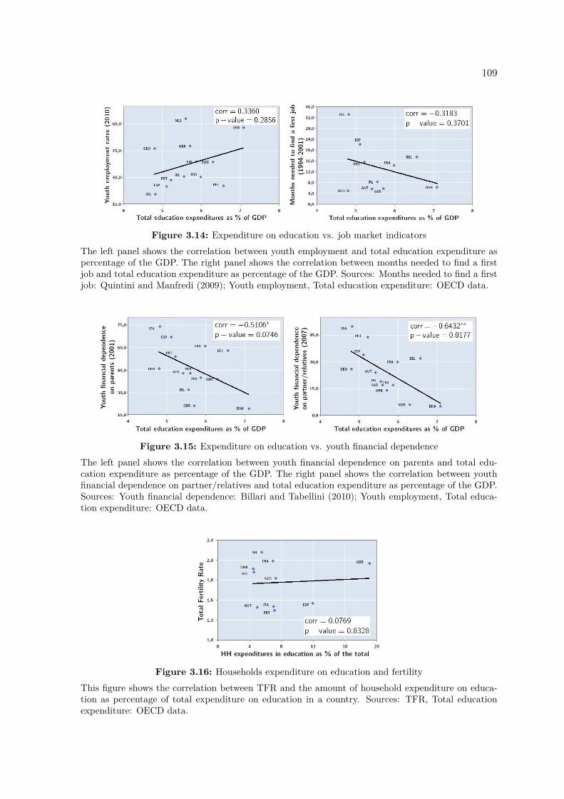
109
Figure 3.14: Expenditure on education vs. job market indicatorsThe left panel shows the correlation between youth employment and total education expenditure aspercentage of the GDP. The right panel shows the correlation between months needed to find a firstjob and total education expenditure as percentage of the GDP. Sources: Months needed to find a firstjob: Quintini and Manfredi (2009); Youth employment, Total education expenditure: OECD data.
Figure 3.15: Expenditure on education vs. youth financial dependenceThe left panel shows the correlation between youth financial dependence on parents and total edu-cation expenditure as percentage of the GDP. The right panel shows the correlation between youthfinancial dependence on partner/relatives and total education expenditure as percentage of the GDP.Sources: Youth financial dependence: Billari and Tabellini (2010); Youth employment, Total educa-tion expenditure: OECD data.
Figure 3.16: Households expenditure on education and fertilityThis figure shows the correlation between TFR and the amount of household expenditure on educa-tion as percentage of total expenditure on education in a country. Sources: TFR, Total educationexpenditure: OECD data.


Chapter 4
Family Ties, Institutions, and Income
Inequality

113
4.1 Introduction
Several cross-country governance indicators show that there is a large heterogeneity in the
quality of regulation and in the effectiveness of institutions, even across European Union
countries (Table 1). These indicators suggest that the implementation of reforms can be
obstructed, even if these reforms aim at reducing corruption, promoting merit and eventually
economic growth (see e.g. Acemoglu, Johnson, and Robinson 2005). Why this can happen
is a crucial economic question. In this paper we address the issue whether the strength of
family ties can affect the quality of the institutional framework of a country.
We tackle this question in a theoretical model in which parents care about the future
utility of their children and - crucial - they can exploit their connection with the political
environment to provide them with private benefits. We assume that parents are heterogeneous
in their political influence, with a higher parental influence implying a lower cost of exerting
the lobbying effort that leads to the acquisition of private benefits. Private benefits, however,
subtract resources from the production of a public good - which we use as a proxy for the
quality of the institutional framework of a country.
The main analysis relies on a comparative static exercise that examines how the equilibrium
outcomes, in particular the public good provision and the income distribution, vary across
economies that differ in the degree of parental altruism - which we use as a proxy for the
strength of family ties.
The theoretical mechanism that this paper highlights can be considered as follows. In the
model, parents can exert a costly lobbying effort that provides their children with a private
benefit. As agents are atomistic, no one feels that her lobbying effort can influence the amount
of public good produced. Thus, in the optimum, a parent chooses the level of effort such that
its marginal cost equals its marginal return - i.e. the marginal increase in private benefit
obtained by her child. The consequence is that at the aggregate level each agent generates a
negative externality that results in the underprovision of the public good. If the economy is
characterized by stronger family ties, we assume that a parent weighs more the future utility
of her child. Consequently, she is willing to exert a larger effort in order to provide her child
with a larger private benefit. At the aggregate level, the higher the degree of altruism, the
more the public resources diverted towards private benefits, and hence the less are available
for the production of the public good - which level is consequently lower. Therefore, the first
main prediction of the model is that stronger family ties are negatively associated with the

114 CHAPTER 4. FAMILY TIES, INSTITUTION, AND INCOME INEQUALITY
Table 4.1: Worldwide Governance Indicators (WGI)
Governance Indicators (2008)Voice and Political Government Regulatory
Rule of LawControl of
Accountability Stability Effectiveness Quality Corruption
EU-15 + NORAUT 1.36 1.30 1.71 1.64 1.92 1.82BEL 1.37 0.61 1.36 1.48 1.38 1.35DNK 1.48 1.00 2.19 1.86 1.92 2.32FIN 1.48 1.36 1.95 1.58 1.87 2.34FRA 1.24 0.58 1.54 1.25 1.40 1.43DEU 1.34 1.08 1.65 1.46 1.72 1.77GRC 0.88 0.32 0.56 0.81 0.75 0.10IRL 1.40 1.16 1.61 1.91 1.74 1.76ITA 0.96 0.41 0.39 0.95 0.43 0.13LUX 1.50 1.52 1.65 1.71 1.82 2.02NLD 1.53 0.95 1.86 1.75 1.76 2.19NOR 1.53 1.33 1.95 1.34 1.96 1.88PRT 1.19 1.05 1.05 1.12 1.02 1.08ESP 1.12 -0.03 0.99 1.27 1.16 1.18SWE 1.53 1.13 1.99 1.68 1.90 2.24UK 1.33 0.56 1.74 1.79 1.68 1.77
The Worldwide Governance Indicators are provided by the World Bank and based on survey data (seeKaufmann, Kraay, and Mastruzzi 2009). A higher number corresponds to a better score.
provision of the public good.
Family ties have another important effect too. When less resources are available for the
public good, the basic wage paid to workers employed in its production is lower as well.
Hence, a higher degree of parental altruism is also associated with a lower basic wage. At
the same time, it leads to a larger total amount of resources diverted towards private ben-
efits. However, the allocation of private benefits is unequal across worker and depends on
the parental political influence. Consequently, the income of workers whose parents are suffi-
ciently influential - hence able to provide their children with large private benefits - is larger
if the degree of parental altruism is higher, while the opposite relationship holds for the other
workers. Therefore, the second main prediction of the model is that stronger family ties are
positively associated with income inequality.
In Section 4 we argue that these results are consistent with stylized evidence from Euro-
pean countries. In particular, Figure 4.1 considers the strength of family ties - as measured
by the World Value Survey first used by Alesina and Giuliano (2010) - versus measures of the
effectiveness of institutions provided by the most recent update of the World Governance In-
dicators provided by the World Bank. European countries characterized by a higher strength
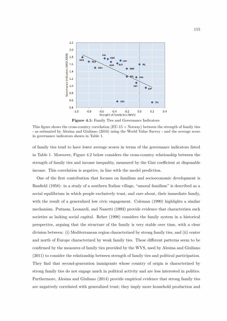
115
Figure 4.1: Family Ties and Governance IndicatorsThis figure shows the cross-country correlation (EU-15 + Norway) between the strength of family ties- as estimated by Alesina and Giuliano (2010) using the World Value Survey - and the average scorein governance indicators shown in Table 1.
of family ties tend to have lower average scores in terms of the governance indicators listed
in Table 1. Moreover, Figure 4.2 below considers the cross-country relationship between the
strength of family ties and income inequality, measured by the Gini coefficient at disposable
income. This correlation is negative, in line with the model prediction.
One of the first contribution that focuses on familism and socioeconomic development is
Banfield (1958): in a study of a southern Italian village, “amoral familism” is described as a
social equilibrium in which people exclusively trust, and care about, their immediate family,
with the result of a generalized low civic engagement. Coleman (1990) highlights a similar
mechanism. Putnam, Leonardi, and Nanetti (1993) provide evidence that characterizes such
societies as lacking social capital. Reher (1998) considers the family system in a historical
perspective, arguing that the structure of the family is very stable over time, with a clear
division between: (i) Mediterranean region characterized by strong family ties, and (ii) center
and north of Europe characterized by weak family ties. These different patterns seem to be
confirmed by the measures of family ties provided by the WVS, used by Alesina and Giuliano
(2011) to consider the relationship between strength of family ties and political participation.
They find that second-generation immigrants whose country of origin is characterized by
strong family ties do not engage much in political activity and are less interested in politics.
Furthermore, Alesina and Giuliano (2014) provide empirical evidence that strong family ties
are negatively correlated with generalized trust; they imply more household production and

116 CHAPTER 4. FAMILY TIES, INSTITUTION, AND INCOME INEQUALITY
less participation in the labor market of women, young adult, and elderly. They are correlated
with lower engagement in political activities and labor market regulation and welfare systems
based upon the family rather than the market or the government. To some extent, these
results are consistent with the theoretical channel highlighted here.
Our framework is related to the literature analyzing the provision of public goods (see e.g.
Oakland 1987) and to the literature studying generational policy (see e.g. Kotlikoff 2002).
Although our analysis relies on public sector provision of the public good, it highlights an
inefficiency that is related - to some extent - to a free riding problem emerging in the context
of private provision of public goods (see Oakland 1987, p. 514-15). As agents are atomistic, no
one feels that, by diverting resources to benefit her own child, she can influence the amount of
public good which will be made available. The consequence is the underprovision of the public
good at the aggregate level. Our model abstracts from the problem of distortionary taxation
in the provision of public goods (introduced by Pigou 1947; see e.g. Stiglitz and Dasgupta
1971 and Atkinson and Stern 1974). As our focus is on a different source of inefficiency, we
assume for simplicity that the amount of taxes collected is exogenous to the model.
The literature studying the impact of institutions on long-run growth is also related to our
work. Some works highlight the importance of considering institutions to be endogenous with
respect to economic outcomes,1 and our approach shares this standpoint. In particular, we
proxy the quality of institutions with the public good provision that is a model equilibrium
outcome.
There are many theories that aim at explaining cross-country differences in institutions and
do not rely on family ties.2 According to the classical view of Becker (1958) and Wittman
(1989), inefficient economic institutions cannot be stable because competition among pressure
groups and political parties will lead to efficient policies and collective choices. By contrast,
Piketty (1995) and Romer (2003) propose models suggesting that economic institutions vary
across countries because of ideological differences. A closer view to our approach suggests
that institutions are chosen by groups that control political power at that time, and not
necessarily in the interest of the whole society. North (1981) provides the first example of
a systematic development of this view. In Acemoglu and Robinson (2006) the elites in the
1See e.g. Acemoglu, Johnson, and Robinson (2005), p. 402 ff., who argue that OLS regressions as those inKnack and Keefer (1995) and Barro (1997) may provide biased estimates of the causal relationship betweeninstitutions and growth because of endogeneity.
2See Acemoglu (2003) and Acemoglu, Johnson, and Robinson (2005) for a comprehensive review of theliterature analyzing this issue.

117
society may have incentive to stop the economic progress in order to maximize the probability
to preserve their power. Our approach is related to this view to the extent that agents diverge
in their political power, i.e. in their capacity of diverting public resources to benefit their
children.
The remainder of this paper is organized as follows. In Section 2, we present the model
setup. In Section 3, we characterize the equilibrium of the economy and the effect of parental
altruism on the production of public good and welfare. Section 4 compares the model predic-
tions to stylized evidence from European countries. Section 5 concludes, discussing limitations
and possible extensions of our analysis.
4.2 Model Setup
4.2.1 Public Good Production, Agents, and Environment
The economy lasts for two periods. In the first period there is a continuum of measure
one of unitary households who make joint decisions,3 each one of them having a child. In
the first period children neither enjoy any utility nor take any decision. In the second period
they become adult, while their parents leave the economy.
In period 1, the government collects an amount of resources T - which is exogenous to
the model, for simplicity. In the second period, the government produces a non-excludable
public good G,4 according to a production function f that employs capital, K, and labor,
L, as inputs. f (K,L) satisfies the Inada conditions. The government aims to maximize the
production of the public good and acts as price taker. For simplicity, the setup abstracts
from the presence of private sector production,5 then G is the only good produced in the
economy in the second period. Consequently, its production employs all workers, who supply
labor inelastically. Wages and capital are obtained from the public resources T .6
Parents are ex-ante heterogeneous in their political influence φ, distributed according to a
cumulative distribution function F (φ), which is common knowledge. Parents are altruistic
towards their children and discount their future utility by b,7 which measures the degree of3In the following, we refer to a unitary household as a “parent.”4G is a public good in the standard sense that “one man’s consumption does not reduce some other man’sconsumption” (Samuelson 1954, 1955).
5Although our focus is on the provision of the public good, this assumption is rather strong and is made forsimplicity. See Section 5 for a more detailed discussion of this assumption and possible extensions.
6The trade-off that we analyze would be still present if only part of the money collected in period 1 is spentin period 2.
7Parents’ utility can be considered as a linear two-period version of the Becker and Barro (1988)’s dynastic

118 CHAPTER 4. FAMILY TIES, INSTITUTION, AND INCOME INEQUALITY
parental altruism.8
In the first period, a parent can exert a lobbying effort e ∈ R+ that generates a private
benefit x(e), with x′ > 0 and x′′ ≤ 0. The private benefit is paid in the next period on the
top of the wage w obtained by her child. Thus, the child’s net income in the next period will
be w + x (e). Exerting an effort e provides a parent with a cost c. The higher the parent’s
political power φ, the lower the cost of effort. The function c(e, φ) is increasing and convex
in e: ce(e, φ) > 0 and cee(e, φ) > 0, while it is decreasing in φ: cφ(e, φ) < 0.9 For simplicity,
we assume that agents have a linear utility function.
Consequently, the utility of a parent of type φ is given by:
Vφ (e) = b [w + x (e) +G]− ce(e, φ). (4.1)
The assumptions on x(e) and c(e, φ) imply the existence of a function e (φ) describing the
optimal effort choice of parents as function of their political influence φ. Define R as the
total amount of the individual private benefits x (e (φ)):
R ≡ˆφx (e (φ)) dF (φ) . (4.2)
Private benefits are diverted from the total resources available for the production of the
public good, T , with R ≤ T . Therefore, the production of the public good must satisfy the
following budget constraint:
K + wL ≤ T −ˆφx (e (φ)) dF (φ) . (4.3)
4.2.2 Timing of the Agents’ Decisions
period-1 Parents of any type simultaneously exert an effort e ≥ 0 maximizing their utility
function Vφ (e).
utility function.8We make the simplifying assumption that all parents in the economy share the same degree of altruismb. Comparative statics over b - our proxy for the strength of family ties - will be considered for thecross-country analysis of the impact of family ties on the quality of institutions.
9The main mechanism is robust to the alternative assumption that a higher parental influence allows toobtain a larger private benefit rather then reducing its cost - that is, x(e, φ) having xe(e, φ) > 0 andxφ(e, φ) > 0, and c(e) having c′ > 0.

119
period-2 Each child inelastically supplies labor, receiving a wage w - determined in equi-
librium - plus a benefit x(e) determined by the effort exerted by her parent in the previous
period.
4.2.3 Functional Forms
To derive closed form solutions we make the following further assumptions.
The parents’ political influence φ is uniformly distributed over the interval[φ, φ
], with
φ, φ > 0. Note that this assumption implies that it is possible to write the total private
benefits as:
R ≡ 1φ− φ
ˆ φ
φx (e (φ)) dφ.
The cost of effort exerted by a parent of type φ is given by:
c(e, φ) = e2
2φ.
The private benefit function x (e) is linear in e:
x (e) = ηe,
with η > 0. Below we set an upper-bound in the degree of altruism b that always guarantees
a unique internal solution for the parental effort choice.10
Furthermore, the technology used for the production of the public good is a Cobb-Douglas
function:
f (K,L) = AKαL1−α,
with 0 < α < 1.
4.2.4 Definition of the Equilibrium
The definition of a competitive equilibrium for the economy is described as follows.
In equilibrium:
1. In period 1, every parent of any type φ ∼ U(φ, φ
)sets effort e to maximize the objective
function (4.1), given the wage w and the public good G determined in period 2.
2. In period 2, the wage w and the public good provision G are determined such that the10See the proof of Proposition 1 in the appendix for more details.

120 CHAPTER 4. FAMILY TIES, INSTITUTION, AND INCOME INEQUALITY
following conditions hold:
(i) children inelasically supply labor, LS (w) = 1;
(ii) the government sets capital K and labor L to maximize the public good provision
G = f (K,L) under the budget constraint (4.3), acting as price taker;
(iii) labor market clears, that is LD(w) = LS(w).
4.3 Results
This section characterizes the equilibrium of the economy described, starting from the
second period. The government maximizes her objective function:
f (K,L) = AKαL1−α,
under the budget constraint (4.3). The supply of labor is inelastic. The equilibrium wage,
capital and production are characterized by the following Lemma.11
Lemma 1 In equilibrium, given the inelastic supply of labor LS(w) = 1, the basic wage is:
w = (1− α) (T −R) .
the capital employed in the production is:
K = α (T −R) ,
hence the public good production is:
G = A [α (T −R)]α .
Proof See the appendix.
In the first period, a parent of type φ chooses the level of effort e by solving the following
11Note that, by contrast with standard general equilibrium framework, the equilibrium wage does not dependon the total factor productivity parameter A. The reason is the following. As the good is public and isnot sold on the market, the resources used to remunerate labor are independent of the level of productionand only determined by the budget constraint. See the proof of Lemma 1 for more details.

121
maximization problem:
maxe∈R+
Vφ (e) = b [w + ηe+G]− e2
2φ.
The optimal parental effort determines the income of children as characterized by the follow-
ing proposition.
Proposition 1 Assume that b ∈[0, T
η2E(φ)
]. Then the utility maximization problem of a
parent of type φ has the following unique solution:
e (φ) = bηφ, (4.4)
and a child whose parent is of type φ obtains in the second period a total income equal to:
w + x(φ) = (1− α)(T − bη2E (φ)
)+ bη2φ. (4.5)
Proof See the appendix.
The equation (4.4) above shows that the optimal parental effort is an increasing function
of the parental political influence. Consequently, the higher the parental’s type φ, the larger
the private benefit that a child obtains - as shown by equation (4.5). A crucial feature of the
model is that a parent, as atomistic, cannot internalize the negative impact of her choice on
the production of the public good in the next period. In other words, no agent feels that,
by diverting resources to benefit her own child, she can influence the amount of public good
which will be made available in the following period. The consequence is that each agent
generates a negative externality that, at the aggregate level, will result in the underprovision
of the public good and in the reduction of the basic wage that the government pays to workers.
4.3.1 Parental Altruism, Public Good Provision and Income Distribution
The rest of this section contains the main analysis, in which we analyze how equilibrium
outcomes vary across economies that differ in the degree of parental altruism.
Proposition 1 already shows the conflicting effects of a higher degree of parental altruism.
At the individual level, φ constant, the higher the degree of altruism, the larger the parental
effort, and hence the larger the private benefit obtained by a child in the second period.
However, at the aggregate level, a higher degree of altruism implies that the basic wage paid
to workers w is lower.

122 CHAPTER 4. FAMILY TIES, INSTITUTION, AND INCOME INEQUALITY
Moreover, larger private benefits implies that a larger share of resources are diverted from
the capital used for the public good production. In particular, the capital employed in the
public good production in the second period as function of the degree of parental altruism is
given by:
K (b) = α(T − bη2E (φ)
),
and hence the amount of public good produced is given by:
G(b) = A[α(T − bη2E (φ)
)]α.
The equations above show that, in equilibrium, the production of the public good, as well as
the basic wage paid to workers, are lower if the degree of parental altruism is higher. The
intuition is the following. In the optimum, a parent chooses a level of effort such that its
return - in terms of future utility of her child - equals the cost of exerting it. If the degree
of altruism is higher, then a parent values more the future utility of her child. Consequently,
she is willing to exert a larger effort in order to provide her child with larger private benefits.
However, as atomistic, this parent does not internalize the negative impact of her choice
on the aggregate equilibrium outcomes, although they can have a direct negative impact
on the future utility of her own children too. At the aggregate level, the higher the degree
of altruism, the more the public resources diverted towards private benefits, and hence the
less those available for the production of the public good: both the employable capital and
wages paid will be lower. By contrast, the maximum levels of basic wage and public good
production are attained in those economies in which the degree of altruism is minimal and
no resources are diverted towards private benefits.
Therefore, the first main prediction of the model is that economies with a higher parental
altruism are characterized by a larger amount of public resources diverted towards private
benefits, hence a lower level of public good provision - because of the higher parents’ willing-
ness to exert effort in order to provide their children with private benefits.
The following proposition underlines this result and analyzes how the total welfare of
children in the second period varies across economies characterized by different levels in the
degree of parental altruism.12
12Measuring the welfare of parents in the first period would allow to consider an additional deadweight lossdue to the effort exerted. However, the use of this measure can lead to a misleading welfare comparisonacross economies that differ in b, given that the utility of parents also changes with b - while the utility ofchildren does not.
123
Proposition 2 Ceteris paribus, if the degree of altruism is higher, the equilibrium produc-
tion of public good is lower:
G(b) = A[α(T − bη2E (φ)
)]α.
Define TW (b) as the total welfare of children in the second period, as function of the
degree of parental altruism, TW (b) = W (b) + R (b) + G (b). There is a threshold A ≡
α−α(T − bη2E (φ)
)1−α in the total factor productivity parameter such that:
(i) if A ≥ A, then TW (b) is maximal at b = 0 and is decreasing in b, for any b ∈(b, Tη2E(φ)
];
(ii) if A < A, then TW (b) is increasing for b ∈[0, b), is maximal if b = b, then is decreasing
for b ∈(b, Tη2E(φ)
]with 0 < b < T
η2E(φ) .
Proof See the appendix.
Therefore, only if the technology employed in the production of the public good is suf-
ficiently inefficient (A < A), then a positive degree of parental altruism in the economy is
beneficial for the total welfare in the second period. Otherwise, the smaller the degree of al-
truism, the higher the total welfare in the economy, because of a smaller amount of resources
diverted from the public good production. However, the heterogeneity in parental political
influence implies that in the second period, in any economy where b > 0, private benefits
and hence total income are different across workers. This feature makes it is interesting to
compare economies beyond a total welfare analysis and consider how the income distribution
varies with differences in the degree of altruism.
Define Iφ(b) as the equilibrium disposable income of a worker whose parent is of type φ.
It is given by the sum of the basic wage and the private benefit, Iφ(b) = w (b) + xφ (b). The
following proposition characterizes how the income distribution vary across economies that
differ in the degree of parental altruism.
Proposition 3 If the degree of parental altruism is larger, then the income distribution is
more unequal, i.e. its variance V (Iφ(b)) is larger. In particular, there is a threshold in the
parental type, φ ≡ E (φ) (1− α), such that:
(i) among workers whose parents are of type φ < φ, the disposable income Iφ(β) is lower if
the degree of parental altruism is higher;

124 CHAPTER 4. FAMILY TIES, INSTITUTION, AND INCOME INEQUALITY
(ii) among workers whose parents are of type φ > φ, the disposable income Iφ(β) is higher if
the degree of parental altruism is higher.
Proof See the appendix.
Proposition 3 shows that the degree of parental altruism has asymmetrically affects income
across workers. Agents whose parents are sufficiently influential (φ > φ) obtain a larger
income if the degree of altruism is higher, thanks to larger private benefits. By contrast, the
net income of agents whose parents have an insufficient political influence (φ ≤ φ) is lower
if the degree of altruism is higher, because of a lower basic wage. Therefore, a second main
prediction of the model is that a higher degree of altruism in the economy implies a larger
income inequality.
4.4 Model Predictions vs. Data
In this next section, we analyze the two main model predictions - (i) a cross-country
negative relationship between the degree of parental altruism and the production of public
good, and (ii) a cross-country positive relationship between the degree of parental altruism
and income inequality - in comparison with stylized evidence from European countries. In
the next section, we discuss the limits of our analysis and possible extensions.
In the model, a higher degree of parental altruism is associated with a higher parents’
effort to provide their children with private benefit. This leads to a larger amount of resources
diverted from the production of the public good, whose level is consequently lower. Therefore,
the first main prediction of the model is a negative cross-country relationship between the
degree of parental altruism and the production of public good. The degree of parental altruism
can be considered as a proxy for the strength of family ties, and the level of public good
production as a proxy for the quality of the institutional framework. Figure 4.1 above shows
that this prediction is consistent with European data. Countries displaying stronger family
ties (as estimated in Alesina and Giuliano 2010 by using the World Value Survey) tend to
have a smaller average score in the Governance Indicators, provided in Table 1.
In our framework, the degree of parental altruism also affects the income distribution.
When the resources used in the production of the public good are lower, the basic wage paid
to workers is lower as well. Therefore, a higher degree of parental altruism is associated
with a lower basic wage. By contrast, it is also associated with a larger total amount of

125
Figure 4.2: Family Ties and Gini at Disposable IncomeThis figure shows the cross-country correlation (EU-15 + Norway) between the strength of family ties- as estimated by Alesina and Giuliano (2010) using the World Value Survey - and the Gini coefficientat disposable income (OECD data).
resources diverted towards private benefits. However, the allocation of private benefit is
unequal across worker. In particular, the income of workers whose parents are sufficiently
influential benefits from a higher degree of parental altruism, while the opposite holds for
all the other workers. Therefore, the second main prediction of the model is a positive
relationship between the degree of parental altruism and income inequality across economies.
Figure 4.2 below shows that also this prediction is supported by evidence from European
countries. Countries displaying stronger family ties tend to show a larger value in the Gini
coefficient at disposable income - an indicator commonly used to measure income inequality.
The first obvious limit of our analysis is strongly related with the type of exercise con-
ducted, namely a comparative statics analysis that considers how equilibrium outcomes vary
with differences in the degree of parental altruism, keeping constant all the other exogenous
variables - in particular, the amount of resources available for public spending, the distribu-
tion of parental political influence, and the return from exerting the lobbying effort. One can
reasonably argue that European countries strongly differ in these dimensions. However, a
comprehensive empirical analysis of this issue is beyond the scope of this paper. Our aim is
to highlight a theoretical channel showing the possibility of a link between parental altruism
and efficient public spending, so helping to explain the observed differences in the quality of
institutions and in income inequality across countries.

126 CHAPTER 4. FAMILY TIES, INSTITUTION, AND INCOME INEQUALITY
4.5 Discussion and Concluding Remarks
This paper provides a simple theoretical framework in which the strength of family ties
affects the quality of institutions and income inequality in a country.
In the model, parents care about their children and can exert a costly lobbying effort
in order to provide them with private benefits. Private benefits are obtained by diverting
resources from the production of a public good. We find a negative relationship between
the degree of parental altruism and the level of production of the public good. Furthermore,
a higher degree of parental altruism implies lower basic wage paid by the government and,
at the same time, more resources that influential parents can divert towards their children.
Consequently, we find a positive relationship between the degree of parental altruism and
inequality in the income distribution.
Although a comprehensive empirical analysis is beyond the scope of this paper and is left
for future research, we argue that the model predictions are in line with stylized evidence
from European countries.
For simplicity, the model setup abstracts from the presence of a private sector in the
economy. We consider interesting to extend the setup such to include the production of a
private good too; then, to allow agents choosing whether to undertake a private sector or a
public sector career - with e.g. the outcome of the first mainly depending on the agent’s skill,
and the outcome of the second being affected by the parental lobbying effort. Besides adding
realism, a similar extension can allow to provide a clearer interpretation of the public good,
as an intermediate public good - e.g. infrastructures - that increases the productivity of the
private sector.
In our framework we further assume that, despite the presence of a cost from exerting
lobbying effort, parents can divert public resources towards private benefits at will. It is
clearly a simplifying assumption, but it crucially affects the model behavior. Therefore, it
would be interesting to augment the model introducing an initial stage in which parents
vote on how public resources will be distributed between: (i) an intermediate public good
that increases private sector productivity, and (ii) a pork-barrel policy. An altruistic parent
would face the following trade-off: on the one side, a larger investment in infrastructures will
increase the private sector productivity and hence the wage of her child if a private sector
worker; on the other side, it will reduce resources available to provide her child with private
benefits if a public sector employee. A higher degree of altruism can provide larger incentives

127
for influential parents to vote for pork-barrel policy, given their comparative advantage in
obtaining private benefits. Therefore, a so-augmented model may still reproduce the main
intuition that is behind the mechanism highlighted by our simpler framework.

128 CHAPTER 4. FAMILY TIES, INSTITUTION, AND INCOME INEQUALITY
4.6 Appendix: Proofs
4.6.1 Proof of Lemma 1
The government produces the public good G solving the following maximization problem:
max f (K,L) = AKαL1−α
s.t. K + wL ≤ T −R.
This problem is equivalent to:
maxL
A (T −R− wL)α L1−α,
which has the following first order condition, necessary and sufficient for an optimum:
−αAw(
L
T −R− wL
)1−α+ (1− α)A
(T −R− wL
L
)α= 0.
Rearranging terms, it is possible to obtain the demand for labor as follows:
LD(w) = (1− α) (T −R)w
.
In equilibrium, labor market clears:
LD(w) = (1− α) (T −R)w
= 1 = LS(w).
Then the equilibrium wage is:
w = (1− α) (T −R) .
the capital employed in the production is:
K = α (T −R) ,
and hence the public good production is:
G = A [α (T −R)]α . �

129
4.6.2 Proof of Proposition 1
Given the cost and the private benefit functions assumed, the utility maximization problem
of a parent of type φ is the following:
max Vφ (e) = b [w + ηe+G]− e2
2φ
s.t. 1φ−φ
´ φφ x (e (φ)) dφ ≤ T
Ignore for the moment the constraint. For any x (e) such that x′ > 0 and x′′ ≤ 0, the
utility function is strictly concave and the first order condition is necessary and sufficient for
a maximum. Rearranging the first order condition, we obtain the unique interior solution:
e (φ) = bφη,
with e (φ) being a function mapping from the parental type φ to the arg max Vφ (e). In
equilibrium, the private benefit obtained by a child whose parent is of type φ is equal to:
x(φ) = bη2φ,
and the total amount of private benefits will be:
R = 1φ− φ
ˆ φ
φbφη2dφ = bη2E (φ) . (4.6)
From the resources constraint, R = bη2E (φ) ≤ T . The expression (4.6) shows that, in
equilibrium, the total amount of private benefits R is linearly increasing in the degree of
altruism b. Then, for any T > 0, there exists a b > 0 such that:
R(b)
= bη2E (φ) = T, (4.7)
with b = Tη2E(φ) being the value of the parental altruism such that the whole public spending
T is diverted towards private benefits.
If b ∈[0, T
η2E(φ)
], then the constraint in the maximization problem is not binding and the
interior solution characterized above is the unique solution of the maximization problem. �

130 CHAPTER 4. FAMILY TIES, INSTITUTION, AND INCOME INEQUALITY
4.6.3 Proof of Proposition 2
The total welfare in the second period is given by:
TW (b) = W (b) +R (b) +G (b)
= (1− α)(T − bη2E (φ)
)+ bη2E (φ) +A
[α(T − bη2E (φ)
)]αDifferentiating TW (b) with respect to b, we obtain:
∂TW (b)∂b
= αη2E (φ)[1− ααA
(T − bη2E (φ))1−α
],
which has infinitely negative slope as b approaches the upper-bound Tη2E(φ) .
The second derivative:
∂2TW (b)∂b2
= −(1− α)α1+αη4E (φ)2A
(T − bη2E (φ))2−α < 0,
shows that the function is concave over the interval b ∈[0, T
η2E(φ)
].
Thus:
A ≥ A ≡ α−α(T − bη2E (φ)
)1−α⇒ ∂TW (b)
∂b|b=0≤ 0,
then TW (b) is constantly decreasing in b over the interval b ∈[0, T
η2E(φ)
], with its maximum
being attained at b = 0.
By contrast:
A < A ≡ α−α(T − bη2E (φ)
)1−α⇒ ∂TW (b)
∂b|b=0> 0,
then, over the interval b ∈[0, T
η2E(φ)
], TW (b) is maximized at:
b = T − αα
1−αA1
1−α
η2E [φ] ,
where 0 < b < Tη2E(φ) . �

131
4.6.4 Proof of Proposition 3
In equilibrium, the disposable income of an agent whose parent is of type φ is given by:
Iφ(b) = w (b) + xφ (b)
= (1− α)(T − bη2E (φ)
)+ bη2φ
As φ ∼ U[φ, φ
], then Iφ(b) is also uniformly distributed:
Iφ(β) ∼ U[(1− α)
(T − bη2E (φ)
)+ bη2φ, (1− α)
(T − bη2E (φ)
)+ bη2φ
],
with variance V (Iφ(b)) = 112
[bη2
(φ− φ
)]2, which is increasing in b. Then, b increases
income inequality.
Differentiating Iφ(b) with respect to b, we obtain:
∂Iφ (b)∂b
= η2 [φ− (1− α)E (φ)] R 0
⇔ φ R (1− α)E (φ) ≡ φ.
Then, among agents whose parents have φ > φ, Iφ(b) increases in b, while among agents
whose parents have φ < φ, Iφ(b) increases in b. �


Chapter 5
Bibliography


135
1. Acemoglu, Daron (2003), “Why not a Political Coase Theorem?” Journal of Compar-
ative Economics, 31: 620-52.
2. Acemoglu, Daron, Simon Johnson, and James A. Robinson (2005), Handbook of Eco-
nomic Growth, vol. 1A, chap. 21, edited by Philippe Aghion and Steven N. Durlauf,
Elsevier, 385–472.
3. Acemoglu, Daron and James A. Robinson (2006), “Economic Backwardness in Political
Perspective,” American Political Science Review, 100(1): 115-131.
4. Acharya, Viral V., and Sascha Steffen (2013), “The greatest carry trade ever? Under-
standing eurozone bank risks”, NBER Working Paper No. 19039.
5. Adsera, Alicia (2004), “Changing Fertility Rates in Developed Countries: The Impact
of Labor Market Institutions,” Journal of Population Economics, 17(1): 17-43.
6. (2005), “Vanishing Children: From High Unemployment to Low Fertility in
Developed Countries,” American Economic Review: Papers and Proceedings, 95(2):
189-193.
7. (2006), “An Economic Analysis of the Gap between Desired and Actual Fertility:
The Case of Spain,” Review of Economics of the Household, 4(1): 75-95.
8. Ahn, Namkee and Pedro Mira (2002), “A Note on the Changing Relationship between
Fertility and Female Employment in Developed Countries,” Journal of Population Eco-
nomics, 14: 505-21.
9. Alesina, Alberto and Paola Giuliano (2010), “The Power of the Family,” Journal of
Economic Growth, 15: 93-125.
10. (2011), “Family Ties and Political Participation,” Journal of the European Eco-
nomic Association, 9(5): 817-839.
11. (2014), “Family Ties,” Handbook of Economic Growth, vol. 2A, ch. 4, edited
by Philippe Aghion and Steven N. Durlauf, Elsevier, 177-215.
12. Altonji, Joseph G. and Charles R. Pierret (2001), “Employer Learning and Statistical
Discrimination,” Quarterly Journal of Economics, 116: 313-500.
13. Atkinson, Anthony B. and Nicholas H. Stern (1974), “Pigou, Taxation and Public
Goods”, Review of Economic Studies, 41: 119-128.
14. Banfield, Edward C. (1958), The Moral Basis of a Backward Society, Free Press, New
York.
15. Barro, Robert J. (1998), Determinants of Economic Growth: A Cross-Country Empir-
ical Study, MIT Press, Cambridge.

136 CHAPTER 5. BIBLIOGRAPHY
16. Barro, Robert J. and Gary S. Becker (1988), “A Reformulation of the Theory of Fer-
tility,” Quarterly Journal of Economics, 103(1): 1-25.
17. (1989), “Fertility Choice in a Model of Economic Growth,” Econometrica, 57:
481-501.
18. Battistini, Niccolò, Marco Pagano, and Saverio Simonelli (2014), “Systemic risk, sovereign
yields and bank exposures in the euro crisis,” Economic Policy, Volume 29, Issue 78,
203-251.
19. Beck, Thorsten, ed. (2012), “Banking Union for Europe, Risks and Challenges,” Centre
for Economic Policy Research, October.
20. Becker, Gary S. (1958), “Competition and Democracy,” Journal of Law and Economics,
1: 105-109.
21. (1960), “An Economic Analysis of Fertility,” in Demographic and Economic
Change in Developed Countries, no. 11 in Universities - National Bureau Conference
Series. Princeton University Press.
22. (1965), “A Theory of the Allocation of Time,” Economic Journal, 75(299):
493-517.
23. Becker, Gary S. and H. Gregg Lewis (1973), “On the Interaction between the Quantity
and Quality of Children,” Journal of Political Economy, 81(2), S279-S288.
24. Benmelech, Efraim, and Nittai K. Bergman (2009), “Collateral Pricing,” Journal of
Financial Economics, 91(3): 339-360.
25. (2011), “Bankruptcy and the Collateral Channel,” Journal of Finance, 66(2):
337-378.
26. (2012), “Credit Traps,” American Economic Review, 102(6): 3004–3032.
27. Bernanke, Ben, and Mark Gertler (1989), “Agency Costs, Net Worth, and Business
Fluctuations,” American Economic Review, 79(1): 14–31.
28. Bernanke, Ben, Mark Gertler, and Simon Gilchrist (1999), “The Financial Accelerator
in a Quantitative Business Cycle Framework,” in Handbook of Macroeconomics, vol. 1,
chap. 21, edited by John B. Taylor and Michael Woodford, Elsevier, 1341–93.
29. Billari, Francesco C. (2004), “Becoming an adult in Europe: A macro(/ micro)- demo-
graphic perspective,” Demographic Research, SC3 (SC3): 15– 44.
30. Billari, Francesco C. and Guido Tabellini (2010), “Italians Are Late. Does It Matter?”
in Demography and the Economy, ed. by J. B. Shoven, The University of Chicago Press,
Chicago.

137
31. Botero, Juan C., Simeon Djankov, Rafael La Porta, Florencio Lopez-de-Silanes, and
Andrei Shleifer (2004), “The Regulation of Labor,” Quarterly Journal of Economics,
119(4): 1339-1382.
32. Broner, Fernando, Aitor Erce, Alberto Martin, and Jaume Ventura (2014), “Sovereign
Debt Markets in Turbolent Times: Creditor Discrimination and Crowding-Out Effects,”
Journal of Monetary Economics, 61(1): 114-142.
33. Butz, William P. and Michael P. Ward (1979), “The Emergence of Countercyclical U.S.
Fertility,” American Economic Review, 69(3): 318-28.
34. Chetty, Raj and Adam Szeidl (2007), “Consumption Commitments and Risk Prefer-
ences,” Quarterly Journal of Economics, 122(2): 831-877.
35. Cho, In-Koo and David M. Kreps (1987), “Signaling games and stable equilibria,”
Quarterly Journal of Economics, 102(2): 179-221.
36. Coleman, James S. (1990), Foundations of Social Theory, Harvard University Press,
Cambridge, MA.
37. Cour-Thimann, Philippine, and Bernard Winkler (2013), “The ECB’s non-standard
monetary policy measures: The role of institutional factors and financial structure”,
ECB Working Paper Series No. 1528 / April 2013.
38. Da Rocha, José M. and Luisa Fuster (2006), “Why Are Fertility Rates And Female
Employment Ratios Positively Correlated Across O.E.C.D. Countries?” International
Economic Review, 47(4): 1187-1222.
39. Doepke, Matthias (2004), “Accounting for Fertility Decline During the Transition to
Growth,” Journal of Economic Growth, 9(3): 347-383.
40. European Central Bank (2011), “The Monetary Policy of the ECB,” Executive Board
of the ECB.
41. (2012), “A Sectoral Account Perspective of Imbalances in the Euro Area,”
Monthly Bulletin, February, 37–43.
42. (2013), “The Perceived External Financing Gap Indicator for Small and Medium-
Sized Enterprises in the Euro Area”, Monthly Bulletin, August.
43. Farber, Henry S. and Robert Gibbons (1996), “Learning and Wage Dynamics,” Quar-
terly Journal of Economics, 111: 1007-1047.
44. Fahr, Stephan, Roberto Motto, Massimo Rostagno, Frank Smets, and Oreste Tristani
(2011), “Lessons for monetary policy strategies from the recent past,” in Approaches to

138 CHAPTER 5. BIBLIOGRAPHY
monetary policy revisited: Lessons from the crisis, edited by Marek Jarociñski, Frank
Smets and Christian Thimann, ECB, 26-66.
45. Giannone, Domenico, Michele Lenza, Huw Pill, and Lucrezia Reichlin (2012), “The
ECB and the Interbank Market,” Economic Journal, 122(564): F467-F486.
46. Goyal, Rishi, Petya K. Brooks, Mahmood Pradhan, Thierry Tressel, Giovanni Dell’Ariccia,
Ross Leckow, and Ceyla Pazarbazioglu (2013), “A Banking Union for the Euro Area,”
IMF Staff Discussion Note 13/1.
47. Hart, Oliver, and John Moore (1988), “Incomplete Contracts and Renegotiation,”
Econometrica, 56, 755-85.
48. (1989), “Default and Renegotiation: A Dynamic Model of Debt,” MIT Working
Paper No. 520, Cambridge, MA.
49. (1994), “A Theory of Debt Based on the Inalienability of Human Capital,”
Quarterly Journal of Economics, 109(4): 841–79.
50. (1998), “Default and Renegotiation: A Dynamic Model of Debt,” Quarterly
Journal of Economics, 113(1): 1–41.
51. Jones, Larry E., Alice Schoonbroodt, and Michèle Tertilt (2010), “Fertility Theories:
Can They Explain the Negative Fertility-Income Relationship?” in Demography and
the Economy, ed. by J. B. Shoven, The University of Chicago Press, Chicago.
52. Kaufmann, Daniel, Aart Kraay, and Massimo Mastruzzi (2009), “Governance Matters
VIII. Aggregate and Individual Governance Indicators 1996-2008,” Policy Research
Working Papers, The World Bank.
53. Kiyotaki, Nobuhiro, and John Moore (1997), “Credit Cycles,” Journal of Political Econ-
omy, 105(2): 211–48.
54. Knack, Stephen and Keefer, Philip (1995), “Institutions and Economic Performance:
Cross-Country Tests Using Alternative Institutional Indicators,” Economics and Poli-
tics, 7(3): 207-228.
55. Kotlikoff, Laurence J. (2002), “Generational Policy,” Handbook of Public Economics,
Vol. 4, 1873-1932.
56. Lane, Philip R. (2012), “The European Sovereign Debt Crisis,” Journal of Economic
Perspectives, 26(3): 49-68.
57. Livshits, Igor, and Koen Schoors (2009), “Sovereign Default and Banking,” BEROC
Working Paper Series.
139
58. Mailath, George J. (1987), “Incentive Compatibility in Signaling Games with a Con-
tinuum of Types,” Econometrica, 55(6): 1349-65.
59. Manuelli, Rodolfo E. and Ananth Seshadri (2009), “Explaining International Fertility
Differences,” Quarterly Journal of Economics, 124(2): 771-807.
60. Mas-Colell, Andreu, Michael D. Whinston, and Jerry R. Green (1995), Microeconomic
Theory, Oxford University Press.
61. Mincer, Jacob (1962), “Labor Force Participation of Married Women,” in H.G. Lewis,
ed., Aspects of Labor Economics. Princeton University Press.
62. (1963), “Market Prices, Opportunity Costs, and Income Effects,” in Measure-
ment in Economics: Studies in Mathematical Economics in Honor of Yehuda Grundeld,
ed. by C.C. et al., pp. 67-82. Stanford University Press, CA.
63. Mishkin, Frederic (2011), “Monetary policy strategy: lessons from the crisis”, in Ap-
proaches to monetary policy revisited: Lessons from the crisis, edited by Marek Jaro-
ciñski, Frank Smets and Christian Thimann, ECB, 67-118.
64. Noldeke, Georg and Eric Van Damme (1990), “Signalling in a Dynamic Labour Market,”
Review of Economic Studies, 57(1): 1-23.
65. North, Douglass C. (1981), Structure and Change in Economic History, W.W. Norton
& Co., New York.
66. Oakland, William H. (1987), “Theory of Public Goods,” Handbook of Public Economics,
Vol. 2, 485-535.
67. Pigou, Arthur C. (1947), A Study in Public Finance, 3rd ed., McMillan, London.
68. Piketty, Thomas (1995), “Social Mobility and Redistributive Politics,” Quarterly Jour-
nal of Economics, 100: 551-84.
69. Putnam, Robert D., Robert Leonardi, and Raffaella Y. Nanetti (1993), Making Democ-
racy Work: Civic Traditions in Modern Italy, Princeton University Press, Princeton.
70. Quintini, Glenda and Thomas Manfredi (2009), “Going Separate Ways? School-to-
Work Transitions in the United States and Europe,” OECD Social, Employment and
Migration Working Papers, No. 90, OECD Publishing.
71. Reher, David S. (1998), “Family Ties in Western Europe: Persistent Contrast,” Popu-
lation and Development Review, 24: 203-234.
72. Riley, John G. (2001), “Silver Signals: Twenty-Five Years of Screening and Signaling,”
Journal of Economic Literature, Vol. XXXIX, 432–478.

140 CHAPTER 5. BIBLIOGRAPHY
73. Romer, David (2003), “Misconceptions and Political Outcomes,” Economic Journal,
113: 1-20.
74. Rothschild, Michael and Joseph E. Stiglitz (1976), “Equilibrium in Competitive In-
surance Markets: An Essay on the Economics of Imperfect Information,” Quarterly
Journal of Economics, 90(4): 630-49.
75. Samuelson, Paul A. (1954), “The Pure Theory of Public Expenditure,” Review of Eco-
nomics and Statistics, 36: 378-389.
76. (1955), “Diagrammatic Exposition of a Theory of Public Expenditure,” Review
of Economics and Statistics, 37: 350-356.
77. Santos, Cezar and David Weiss (2011), “Why Not Settle Down Already? A Quantitative
Analysis of the Delay in Marriage,” Working Paper, University of Pennsylvania.
78. Shleifer, Andrei, and Robert W. Vishny (1992), “Liquidation Values and Debt Capacity:
A Market Equilibrium Approach,” Journal of Finance, 47(4): 1343–66.
79. Sobel, Joel (2009), “Signaling games,” Encyclopedia of Complexity and Systems Science,
R. Meyers (ed.), 8125-8139.
80. Sommer, Kamila (2011), “Fertility Choice in a Life Cycle Model with Idiosyncratic
Uninsurable Earnings Risk,” Working Paper, Georgetown University.
81. Spence, A. Michael (1973), “Job market signaling,” Quarterly Journal of Economics,
87: 355-74.
82. Stiglitz, Joseph E. and Partha S. Dasgupta (1971), “Differential Taxation, Public
Goods, and Economic Efficiency,” Review of Economic Studies, 38: 151-174.
83. Uhlig, Harald (2013), “Sovereign Default Risk and Banks in a Monetary Union,” NBER
Working Paper No. 19343.
84. Venn, Danielle (2011), “Earnings Volatility and its Consequences for Households,”
OECD Social, Employment and Migration Working Papers, No. 125, OECD Pub-
lishing.
85. Wehinger, Gert (2013), “SMEs and the Credit Crunch: Current Financing Difficulties,
Policy Measures and a Review of Literature,” OECD Journal: Financial Market Trends,
Volume 2013/2.
86. Wilson, Charles A. (1977), “A Model of Insurance Markets with Incomplete Informa-
tion,” Journal of Economic Theory, 16(2): 167-207.
87. Wittman, Donald (1989), “Why Democracies Produce Efficient Results,” Journal of
Political Economy, 97: 1395-424.

Eidesstattliche Erklärung
Hiermit erkläre ich, die vorliegende Dissertation selbstständig angefertigt und mich keiner
anderen als den in ihr angegebenen Quellen und Hilfsmitteln bedient zu haben. Insbesondere
sind sämtliche Zitate aus anderen Quellen als solche gekennzeichnet und mit Quellenangaben
versehen.
Mannheim, Juli 2015 Giuseppe Corbisiero
141


Curriculum Vitae
2010-2015 Ph.D. in Economics
Center for Doctoral Studies in Economics,
University of Mannheim
2009-2010 Master in Economics and Finance (MEF)
University of Naples Federico II
2006-2009 Laurea Specialistica (M.Sc.) in Economics
University of Naples Federico II
2002-2006 Laurea Triennale (B.A.) in Economics
University of Naples Federico II
143