Infinite-Dimensional Lie Theory for Gauge Groups · Acknowledgement I would like to express my...
184
Infinite-Dimensional Lie Theory for Gauge Groups Vom Fachbereich Mathematik der Technischen Universit¨ at Darmstadt zur Erlangung des Grades eines Doktors der Naturwissenschaften (Dr. rer. nat.) genehmigte Dissertation von Dipl.-Math. Christoph Wockel aus Kassel Referent: Prof. Dr. Karl-Hermann Neeb Korreferent: Prof. Dr. Peter Michor Tag der Einreichung: 12.07.2006 Tag der m¨ undlichen Pr¨ ufung: 20.10.2006 Darmstadt 2006 D17
Transcript of Infinite-Dimensional Lie Theory for Gauge Groups · Acknowledgement I would like to express my...
Infinite-Dimensional Lie Theoryfor Gauge Groups
Vom Fachbereich Mathematik
der Technischen Universitat Darmstadt
zur Erlangung des Grades eines Doktors der
Naturwissenschaften (Dr. rer. nat.) genehmigte
Dissertation
von
Dipl.-Math. Christoph Wockel
aus Kassel
Referent: Prof. Dr. Karl-Hermann Neeb
Korreferent: Prof. Dr. Peter Michor
Tag der Einreichung: 12.07.2006
Tag der mundlichen Prufung: 20.10.2006
Darmstadt 2006D17

To my parents
for teaching me poems and fishes
Danksagung
An dieser Stelle mochte ich mich bei den Personen bedanken, die mich wahrendmeiner Zeit als Doktorand unterstutzt haben.Zunachst mochte ich mich bei meinem Doktorvater, Prof. Dr. Karl-HermannNeeb fur eine vorbildliche Betreuung wahrend der gesamten Zeit bedanken. Siewar gepragt von außerordentlicher wissenschaftlicher Kompetenz, einer prak-tisch standigen Ansprechbarkeit, einem sehr guten personlichen Verhaltnis undvielfaltigen Moglichkeiten zur wissenschaftlichen Weiterentwicklung.
Des weiteren mochte ich mich bei den Mitgliedern der Arbeitsgruppe Algebra,Geometrie und Funktionalanalysis des Fachbereichs Mathematik der TechnischenUniversitat Darmstadt bedanken, die einen wesentlichen Anteil an der Entste-hung dieser Dissertation hatten. Insbesondere mochte ich Christoph Muller furdie gute Zusammenarbeit bei allen auftauchenden Fragen und fur das haufige Ko-rrekturlesen, sowie Helge Glockner fur die vielfaltige wissenschaftliche Beratungdanken. Fur die Unterstutzung bei der Erledigung des zum Teil recht großenorganisatorischen Aufwands wahrend einer solchen Promotionszeit sei an dieserStelle außerdem Gerlinde Gehring ausdrucklich gedankt. Ferner mochte ich dergesamten Arbeitsgruppe fur das angenehme Arbeitsklima danken.
Die zum Teil sehr großen privaten Entbehrungen, die unweigerlich miteiner Promotion verbunden sind, hat meine Frau Melanie immer mit großerUnterstutzung fur meine beruflichen Vorhaben erwidert. Ihr mochte ich andieser Stelle fur das aufgebrachte Verstandnis und die vielfaltige moralische Un-terstutzung danken.
Bei der Technischen Universitat Darmstadt mochte ich mich ferner fur dieFinanzierung meines Promotionsprojekts durch ein Doktorandenstipendium be-danken.
iv
Acknowledgement
I would like to express my gratitude to the people who supported me duringmy time as a Ph.D. student. First of all I want to thank my advisor, Prof. Dr.Karl-Hermann Neeb, for his exemplary supervision during the entire time – forhis constant availability, outstanding scientific expertise, a very good personalrelationship, and active support of my scientific growth.
Furthermore, I want to express my thanks to those members of the researchgroup Algebra, Geometry and Functional Analysis at the mathematics departmentof the Technical University of Darmstadt who had an essential part in the formationof this thesis. In particular, I want to thank Christoph Muller for collaboration inall respects and for extensive proof reading, as well as Helge Gockner for frequentconsultation. For help in all administrative efforts during the work on this thesisI want to express my gratitude to Gerlinde Gehring. Further, I thank the wholegroup for a friendly working atmosphere.
The great gap that was left in my private life during the work on this thesiswas always answered by my wife Melanie with ongoing support for my professionalaims. I want to express my deep gratitude for her understanding.
In addition, I would like to thank the Technical University of Darmstadt for adoctoral scholarship for my work.
v
AbstractZiel dieser Arbeit ist die Initialisierung einer Lie-theoretischen Behandlung von
Symmetriegruppen von Hauptfaserbundeln, hauptsachlich von Eichgruppen. Furein fixesK-Hauptfaserbundel P bezeichnen wir diese mit Gau(P) und identifizierensie meistens mit der Gruppen der aquivarianten glatten Abbildungen C∞(P,K)K .Diese Gruppen werden als unendlichdimensionale lokalkonvexe Lie-Gruppen be-handelt. Da unendlichdimensionale Lie-Theorie ein Gebiet ist, das momentaneinem regen Forschugsprozess unterworfen ist und die Terminologie noch nichtgefestigt ist, mussen wir die Fragestellung prazisieren. In dieser Arbeit wird denfolgenden Fragen nachgegangen:
• Fur welche P ist Gau(P) eine unendlichdimensionale Lie-Gruppe?
• Wie konnen die Homotopiegruppen πn(Gau(P)) bestimmt werden?
• Wie sieht die Erweiterungstheorie von Gau(P) aus?
Dies ist naturlich nur ein kleiner Teil der Fragen, die mit Lie-Gruppen ver-bunden sind. Sie konnen alle mit der gleichen Idee behandelt werden, die wir imFolgenden beschreiben. Ein Bundel kann (bis auf Aquivalenz) auf mehrere ver-schiedenen Arten beschrieben werden. Zwei verschiedene Arten sind durch dieBeschreibung durch eine klassifizierende Abbildung fP und durch einen Kozyk-lus KP gegeben. Eine klassifizierende Abbildung fP ist eine global definierteAbbildung mit Werten in einem klassifizierenden Raum, wahrend ein Kozyklusaus vielen lokal definierten Abbildungen besteht, die Werte in der Lie-GruppeK annehmen und bestimmte Kompatibilitatsbedingungen erfullen. Diese beidenObjekte, klassifizierende Abbildungen und Kozyklen, leben in zwei verschiedenenWelten, namlich Topologie und Lie-Theorie.
Die Idee ist nun, diese beiden Konzepte zu kombinieren und die bestehendenResultate aus Topologie und Lie-Theorie zu benutzen um Antworten auf die obengenannten Fragen zu erhalten. Da diese Fragen recht allgemein gehalten sind kannman nicht erwarten, Antworten in dieser Allgemeinheit zu erhalten. In dieserArbeit werden wir jedoch viele interessante Falle aus der mathematischen Physikbehandeln. Die dabei erzielten Resultate beinhalten:
• Konstruktion einer Lie-Gruppenstruktur auf Gau(P) falls die Struktur-gruppe lokal exponentiell ist.
• Eine kanonische schwache Homotopieaquivalenz Gau(P) → Gauc(P).
• Entwicklung eines Gattungsverfahrens fur Hauptfaserbundel.
• Konstruktion einer Erweiterung Gau(P) → Aut(P) → Diff(M)P .
• Bestimmung einiger Homotopiegruppen und aller rationalen Homotopiegrup-pen von Gau(P) fur endlichdimensionale Hauptfaserbundel uber Spharen.
• Konstruktion zentraler Erweiterungen Z → GP → Gau(P)0.
• Konstruktion einer automorphen Wirkung von Aut(P) auf GP .
• Anwendung auf affine getwistete Kac–Moody Gruppen.
vi
AbstractThe aim of this thesis is to consider symmetry groups of principal bundles
and to initiate a Lie theoretic treatment of these groups. These groups of maininterest are called gauge groups. When taking a particular principal K-bundleP into account, we denote the gauge group of this bundle by Gau(P), which wemostly identify with the space of smooth K-equivariant mappings C∞(P,K)K .These groups will be treated as infinite-dimensional Lie groups, modelled on anappropriate vector space. Since Lie theory in infinite dimensions is a research areawhich is presently under active development, this terminology is not settled, andwe have to make precise what we mean with “infinite-dimensional Lie theory”.The following questions are considered in this thesis:
• For which bundles P is Gau(P) an infinite-dimensional Lie group, modelledon an appropriate locally convex space?
• How can the homotopy groups πn(Gau(P)) be computed?
• What extensions does Gau(P) permit?
Of course, this is only a marginal part of the questions that come along withLie groups. These problems have in common that they can be approached with thesame idea, which we describe now. Along with a bundle P come many differentways of describing it (up to equivalence). Two fundamental different ways aregiven by describing P either in terms of a classifying map fP , or by a cocycle KP .A classifying map fP is a globally defined map fP with values in some classifyingspace, while a cocycle consists of many locally defined maps, with values in a Liegroup, obeying some compatibility conditions. These objects, classifying maps andcocycles, live in two different worlds, namely topology and Lie theory.
The idea now is to combine these two concepts and to use the existing toolsfrom topology and Lie theory in order to give answers to the questions above. Sincethe questions are formulated quite generally, we cannot hope to get answers in fullgenerality, but for many interesting cases occurring in mathematical physics, wewill provide answers. These include:
• Construction of a Lie group structure on Gau(P) if the structure group islocally exponential.
• Showing that the canonical inclusion Gauc(P) → Gau(P) is a weak homo-topy equivalence.
• Providing a smoothing procedure for continuous principal bundles.
• Construction of an Extension of Lie groups Gau(P) → Aut(P) → Diff(M)P .
• Calculation of some homotopy groups and of all rational homotopy groupsof Gau(P) for finite-dimensional principal bundles over spheres.
• Construction of central extensions Z → GP → Gau(P)0.
• Construction of an automorphic action of Aut(P) on GP .
• Applications to affine twisted Kac–Moody groups.
vii

Contents
1 Introduction 1
2 Foundations 7
2.1 Manifolds with corners . . . . . . . . . . . . . . . . . . . . . . . . . 7
2.2 Spaces of mappings . . . . . . . . . . . . . . . . . . . . . . . . . . . 12
2.3 Extensions of smooth maps . . . . . . . . . . . . . . . . . . . . . . 22
3 The gauge group as an infinite-dimensional Lie group 27
3.1 The Lie group topology on the gauge group . . . . . . . . . . . . . 27
3.2 Approximation of continuous gauge transformations . . . . . . . . . 37
3.3 Equivalences of principal bundles . . . . . . . . . . . . . . . . . . . 47
3.4 The automorphism group as an infinite-dimensional Lie group . . . 59
4 Calculating homotopy groups of gauge groups 75
4.1 The evaluation fibration . . . . . . . . . . . . . . . . . . . . . . . . 76
4.2 The connecting homomorphisms . . . . . . . . . . . . . . . . . . . . 84
4.3 Formulae for the homotopy groups . . . . . . . . . . . . . . . . . . 91
5 Central extensions of gauge groups 95
5.1 A central extension of the gauge algebra . . . . . . . . . . . . . . . 95
5.2 Integrating the central extension of the gauge algebra . . . . . . . . 98
5.3 Actions of the automorphism group . . . . . . . . . . . . . . . . . . 109
5.4 Kac–Moody groups . . . . . . . . . . . . . . . . . . . . . . . . . . . 115
A Appendix: Notions of infinite-dimensional Lie theory 125
A.1 Differential calculus in locally convex spaces . . . . . . . . . . . . . 125
A.2 Central extensions . . . . . . . . . . . . . . . . . . . . . . . . . . . 129
A.3 Actions of locally convex Lie groups . . . . . . . . . . . . . . . . . . 132
B Appendix: Notions of bundle theory 137
B.1 Vector- and Principal Bundles . . . . . . . . . . . . . . . . . . . . . 137
B.2 Classification results for principal bundles . . . . . . . . . . . . . . 144
B.3 Connections on principal bundles . . . . . . . . . . . . . . . . . . . 149
ix
x Contents
Bibliography 157
Notation 163
Index 167
Chapter 1
Introduction
Bundle theory and Lie theory are two of the most important topics in MathematicalPhysics. Bundles occur naturally in the description of many physical systems, oftenin terms of (co-) tangent bundles of manifolds or in terms of principal bundles.These descriptions always carry redundant information, emerging from introducingcoordinates or from geometrical realisations. This redundant information gives riseto symmetries of the mathematical description, which can be expressed in termsof groups. In many interesting cases, these groups are geometric objects itself andare called Lie groups.
One of the most popular examples is general relativity, which is formulated interms of manifolds and the curvature of vector bundles. The pioneering idea ofEinstein was that any point and any coordinate system of the manifold shouldhave equal physical laws. This assumption leads to a theory which is invariantunder diffeomorphisms by assumption. Thus general relativity may be viewedas a theory formulated in terms of manifolds M and their tangent bundles TM ,which has the Lie group Diff(M) as symmetry group.
The aim of this thesis is to consider symmetry groups of principal bundlesand to initiate a Lie theoretic treatment of these groups. The groups of maininterest are gauge groups, which can be viewed as the “internal” symmetry groupsof quantum field theories (cf. [MM92] [Na00]). When taking a particular principalbundle P into account, we denote the gauge group of this bundle by Gau(P).These groups will be treated as infinite-dimensional Lie groups, modelled on anappropriate vector space. Since Lie theory in infinite dimensions is a research areawhich is presently under active development, this terminology is not settled, andwe have to make precise what we mean with “infinite-dimensional Lie theory”.The following questions are considered in this thesis:
1
2 Introduction
• For what bundles P is Gau(P) an infinite-dimensional Lie group, modelledon an appropriate locally convex space?
• How can the homotopy groups πn(Gau(P)) be computed?
• What extensions does Gau(P) permit?
Of course, this is only a marginal part of the questions that come along withLie groups. These problems have in common that they can be approached with thesame idea, which we describe now. Along with a bundle P come many differentways of describing it (up to equivalence). Two fundamental different ways aregiven by describing P either in terms of a classifying map fP , or by a cocycle KP .A classifying map fP is a globally defined map fP with values in some classifyingspace, while a cocycle consists of many locally defined maps, with values in a Liegroup, obeying some compatibility conditions. These objects, classifying maps andcocycles, live in two different worlds, namely topology and Lie theory.
The idea now is to combine these two concepts and to use the existing toolsfrom topology and Lie theory in order to give answers to the questions above. Sincethe questions are formulated quite generally, we cannot hope to get answers in fullgenerality, but for many interesting cases occurring in mathematical physics, wewill provide answers.
We now give a rough outline of the results that can be found in this thesis,without going into too much detail. Throughout the thesis, we always assume thatthe base spaces of the bundles under consideration are connected.
Chapter 2: In the first section, we introduce manifolds with corners, which arethe objects that we use extensively throughout the thesis. We have the needto work with these objects, since we are forced to consider compact subsetsof certain open subsets of a manifold as manifolds themselves (e.g., [0, 1]n asa manifold with corners in Rn). Since we want to work with mapping spaces,we take a quite uncommon definition of a manifold with corners, which weshow to be equivalent to the usual one later in the chapter.
In the second section, we introduce mapping spaces and topologies on them.In particular, we define the C∞-topology on spaces of smooth mappingsbetween manifolds, which is the topology we use throughout this thesis.Along with this, we show and recall some basic facts on spaces of smoothmappings with values in locally convex spaces or Lie groups and on spacesof smooth sections in vector bundles. These facts are the Lie theoretic toolsfor mapping spaces, mentioned above, which we use.
In the last section, we relate our concept of a manifold with corners to theone more frequently used in the literature. The results of this section arealso well-known, but we will derive alternative proofs.
Introduction 3
Chapter 3: In this chapter, we introduce Lie group structures on the gauge groupGau(P) and on the automorphism group Aut(P) of a principal bundle P overa compact manifold M . In the first section, we consider the gauge groupGau(P) and introduce a Lie group topology on it under a technical require-ment. This requirement, called “property SUB”, encodes exactly what weneed to ensure the construction of a canonical Lie group topology on Gau(P).
Theorem (Lie group structure on Gau(P)). Let P be a smooth princi-pal K-bundle over the compact manifold M (possibly with corners). If P hasthe property SUB, then Gau(P) ∼= C∞(P,K)K carries a Lie group structure,modelled on C∞(P, k)K. If, moreover, K is locally exponential, then Gau(P)is so.
In the remainder of the section, we discuss the question what bundles havethe property SUB. Most bundles (including all bundles modelled on Banachspaces) have this property.
In the second section, we derive a first major step towards the computationof the homotopy groups πn(Gau(P)) of the gauge group. Following ideasfrom mapping groups, we reduce the determination of πn(Gau(P)) to thecase of continuous gauge transformations Gauc(P).
Theorem (Weak homotopy equivalence for Gau(P)). Let P be asmooth principal K-bundle over the compact manifold M (possiblywith corners). If P has the property SUB, then the natural inclu-sion ι : Gau(P) → Gauc(P) of smooth into continuous gauge transfor-mations is a weak homotopy equivalence, i.e., the induced mappingsπn(Gau(P)) → πn (Gauc(P)) are isomorphisms of groups for n ∈ N0.
This theorem is the first connection between the two worlds described above,i.e., Lie theory (considering Gau(P) as the object of interest) and topology(considering Gauc(P) as the object of interest). It reduces the determinationof πn(Gau(P)) completely to the determination of πn(Gauc(P)), which wewill consider in Chapter 4.
In the third section, we develop the technique of reducing problems for gaugetransformations to problems on Lie group valued mappings, satisfying somecompatibility conditions further, to bundle equivalences. With the aid ofsome technical constructions, we derive the following two theorems, whichare somewhat apart from the main objective of this chapter.
Theorem (Smoothing continuous principal bundles). Let K be a Liegroup modelled on a locally convex space, M be a finite-dimensional para-compact manifold (possibly with corners) and P be a continuous principal
K-bundle over M . Then there exists a smooth principal K-bundle P overM and a continuous bundle equivalence Ω : P → P.
4 Introduction
Theorem (Smoothing continuous bundle equivalences). Let K be aLie group modelled on a locally convex space, M be a finite-dimensionalparacompact manifold (possibly with corners) and P and P ′ be two smoothprincipal K-bundles over M . If there exists a continuous bundle equivalenceΩ : P → P ′, then there exists a smooth bundle equivalence Ω : P → P ′.
Again, these theorems provide an interplay between locally defined Lie groupvalued functions with compatibility conditions on the one hand and classi-fying maps in classifying spaces on the other, because the classical proofof these theorems in the case of finite-dimensional bundles uses classifyingmaps.
The last section of Chapter 3 is a first approach to the extension theory ofGau(P). One way of defining Gau(P) is to consider it as a normal sub-group of Aut(P), i.e., Aut(P) is the extension of some group isomorphic toAut(P)/Gau(P) by Gau(P). By using techniques from the Lie theory ofmapping spaces, we put this into a Lie theoretic context.
Theorem (Aut(P) as an extension of Diff(M)P by Gau(P)). LetP be a smooth principal K-bundle over the closed compact manifold M . IfP has the property SUB, then Aut(P) carries a Lie group structure suchthat we have an extension of smooth Lie groups
Gau(P) → Aut(P)Q
−−− Diff(M)P ,
where Q : Aut(P) → Diff(M) is the canonical homomorphism and Diff(M)Pis the open subgroup of Diff(M) preserving the equivalence class of P underpull-backs.
Chapter 4: In this chapter, we turn to the computation of πn(Gauc(P)), whichwe have seen to be isomorphic to πn(Gau(P)) in Chapter 3. We can thuswork in a purely topological setting and take the existing tools of homotopytheory into account. In the first section, we explain how the problem of thedetermination of Gauc(P) can be expressed in terms of long exact homotopysequences and connecting homomorphisms.
In the second section, we show how the connecting homomorphisms, men-tioned above, can be computed in terms of homotopy invariants of the struc-ture group and the bundle. The crucial tool will be the evaluation fibrationev : Gauc(P) → K, determined uniquely by p0 · ev(f) = f(p0) for some base-point p0. Furthermore, it will turn out that the case of bundles over spheresis the generic one.
Theorem (Connecting homomorphism is the Samelson product).Let K be locally contractible and P be a continuous principal K-bundle over
Introduction 5
Sm, represented by
b ∈ πm−1(K) ∼= [Sm, BK]∗ ∼= Bun(Sm, K).
Then the connecting homomorphisms δn : πn(K) → πn+m−1(K) in the longexact homotopy sequence
· · ·→πn+1(K)δn+1−−→πn+m(K)→πn(Gauc(P))→πn(K)−→ δnπn+m−1(K)→· · ·
induced by the evaluation fibration, are given by δn(a) = −〈b, a〉S, where〈·, ·〉S denotes the Samelson product.
In the last section of Chapter 4, we explain how this exact sequence canbe used to compute πn(Gauc(P)). Since for many questions in infinite-dimensional Lie theory it suffices to know the rational homotopy groupsπQn (Gauc(P)), we focus on πQn (Gauc(P)).
Theorem (Rational homotopy groups of gauge groups). Let K be afinite-dimensional Lie group and P be a continuous principal K-bundle overX, and let Σ be a compact orientable surface of genus g. If X = Sm, then
πQn (Gauc(P)) ∼= πQn+m(K)⊕ πQn (K)
for n ≥ 1. If X = Σ and K is connected, then
πQn (Gauc(P)) ∼= πQn+2(K)⊕ πQn+1(K)2g ⊕ πQn (K)
for n ≥ 1.
Since the rational homotopy groups of finite-dimensional Lie groups areknown, this yields a complete description of the rational homotopy groups ofgauge groups for finite-dimensional bundles with connected structure groupover spheres and compact surfaces.
Chapter 5: In this chapter, we consider the construction of central extensionsof Gau(P) and applications to Kac–Moody groups. In the first section,we consider the construction of a central extension of the gauge algebrag := gau(P), which is motivated by the corresponding construction for triv-ial bundles. This central extension gω is given by a “covariant” cocycleω : g× g → zM(Y ), which is constructed with the aid of some K-invariantbilinear form κ : k× k → Y . The target space zM(Y ) of ω is some locallyconvex space zM(Y ), which depends on Y and on the base manifold M ofthe bundle P under consideration.
In the second and third section, we check the integrability conditions fromthe established theory of central extensions of infinite-dimensional Lie groupsfor the central extension gω. We again encounter the interplay between theLie theoretic properties of Gau(P) and the topological properties of P , whichmake the proof of the following theorem work.
6 Introduction
Theorem (Integrating the central extension of gau(P)). Let P be afinite-dimensional smooth principal K-bundle over the closed compact man-ifold M and κ : k× k → V (k) be universal. Furthermore, set z := zM(V (k)),g := gau(P) and G := Gau(P)0. If ω : g× g → z is the covariant cocycle,then the central extension z → gω g of Lie algebras integrates to an exten-sion of Lie groups Z → G G.
In the third section, we also consider the construction of a canonical actionof the automorphism group Aut(P) of the bundle P on the central extensiongω. This action will become important in the last section, because it is closelyrelated to Kac–Moody algebras and their automorphisms. At the end of thesection, we show that we also get a canonical action of Aut(P) on the central
extension G.
Theorem (Integrating the Aut(P)-action on gau(P)). Let P be afinite-dimensional smooth principal K-bundle over the closed compact man-ifold M and set g := gau(P) and G := Gau(P)0. If ω : g× g → z is the co-
variant cocycle and if Z → G G is the central extension from the preced-ing theorem, then the smooth action of Aut(P) on gω integrates to a smooth
action of Aut(P) on G.
As an application, we describe in the last section of Chapter 5 the relationof the results of the previous chapters to Kac–Moody groups. After makingthe setting of Kac–Moody groups precise, we consider in particular theirhomotopy groups and show how the automorphic action of Aut(P) on gωleads to a geometric description of the automorphism group of twisted loopalgebras. In the end of this section we give an outlook how the results ofthis thesis can be used to construct generalisations of Kac–Moody algebrasand groups.
The thesis is organised as follows. In the beginning of each chapter and section,we give a rough outline of our aims. During each section, we give ongoing commentsthat should motivate the procedure of the section and should illustrate the flow ofideas. Terminology and notation can mostly be found in remarks and definitions,as long as they are important for the sequel.
Relations of the work presented in this thesis to work of other authors (at leastas long as they are known to the author of the thesis), ideas for further researchand open problems can be found at the end of each section and sometimes in themotivating text at the beginning of sections and chapters. However, if we cite aresult directly, we make this explicit at the point of occurrence without repeatingit again at the end of the section.
In the appendix, we present some facts on infinite-dimensional Lie theory andbundle theory, which we often refer to. This presentation is not meant to beexhaustive, it should only make it easier to follow the text by stating some thingsexplicitly instead of referring to the literature.
Chapter 2
Foundations
This chapter presents the underlying material for the following chapters. We shallintroduce manifolds with corners in the first section, which we will need to considerin the topologisation of the gauge group, even for principal bundles over manifoldswithout boundary. The second section provides the facts on spaces of smoothmaps, which we shall use in the sequel. These two concepts, manifolds with cornersand spaces of smooth maps along with their properties, will be the cornerstonesof the theory we will build in the following chapters. Since our definition of amanifold with corners is somewhat uncommon, we relate it to the commonly useddefinition of a manifold with corners in the third and last section.
2.1 Manifolds with corners
In this section we present the elementary notions of differential calculus on locallyconvex spaces for not necessarily open domains and introduce manifolds with cor-ners. Since we are aiming for mapping spaces, we need a notion of differentiabilityinvolving only the values of a given function on its domain without referring toextensions of the map to some open neighbourhood.
The idea, taken from [Mi80], is to restrict attention to maps which are definedon an open and dense subset of its domain, because this determines a continu-ous map completely. It will turn out that with this definition, most ideas frommanifolds without boundary carry over to manifolds with corners, as long as onlytangent mappings and their continuity are involved.
Definition 2.1.1. Let X and Y be a locally convex spaces and U ⊆ X be open.Then f : U → Y is differentiable or C1 if it is continuous, for each v ∈ X thedifferential quotient
df(x).v := limh→0
f(x+ hv)− f(x)
h
exists and if the map df : U ×X → Y is continuous. If n > 1 we inductively definef to be Cn if it is C1 and df is Cn−1 and to be C∞ or smooth if it is Cn. We say
7
8 2. Foundations
that f is C∞ or smooth if f is Cn for all n ∈ N0. We denote the correspondingspaces of maps by Cn(U, Y ) and C∞(U, Y ).
Definition 2.1.2. Let X and Y be locally convex spaces, and let U ⊆ X be aset with dense interior. Then f : U → Y is differentiable or C1 if it is continuous,fint := f |int(U) is C1 and the map
d (fint) : int(U)×X → Y, (x, v) 7→ d (fint) (x).v
extends to a continuous map on U ×X, which is called the differential df of f . Ifn > 1 we inductively define f to be Cn if it is C1 and df is Cn−1. We say that fis C∞ or smooth if f is Cn for all n ∈ N0. We denote the corresponding spaces ofmaps by Cn(U, Y ) and C∞(U, Y ).
Similarly, we introduce holomorphic mappings on non-open domains. We shallnot need this concept very often.
Definition 2.1.3. If X and Y are locally convex complex vector spaces andU ⊆ X has dense interior, then a smooth map f : U → Y is called holomorphic iffint is holomorphic, i.e., if each map dfint(x) : X → Y is complex linear (cf. [Mi84,p. 1027]). We denote the space of all holomorphic functions on U by O(U, Y ) .
Remark 2.1.4. Note that in the above setting df(x) is complex linear for allx ∈ U due to the continuity of the extension of dfint.
We now introduce higher differential of smooth function, which have not beendefined in Definition 2.1.2.
Remark 2.1.5. Since int(U ×Xn−1) = int(U)×Xn−1 we have for n = 1 that(df)int = d (fint) and we inductively obtain (dnf)int = dn (fint). Hence the higherdifferentials dnf are defined to be the continuous extensions of the differentialsdn(fint) and thus we have that a map f : U → X is smooth if and only if
dn (fint) : int(U)×Xn−1 → Y
has a continuous extension dnf to U ×Xn−1 for all n ∈ N.
Of course we have a chain rule, the most important tool in any notion ofdifferential calculus. However, in the way we introduced differentiable maps weneed to assume that mappings are well-behaved with respect to the interiors ofthe domains in order to have a chain rule.
Remark 2.1.6. If f : U1 → U2, g : U2 → Y with f(int(U1)) ⊆ int(U2) are C1,then the chain rule for locally convex spaces [Gl02a, Proposition 1.15] and(g f)int = gint fint imply that g f : U1 → Y is C1 and its differential is givenby d(g f)(x).v = dg(f(x)).df(x).v. In particular, g f is smooth if g and f areso.
2.1. Manifolds with corners 9
With the above definitions and the chain rule in mind, we can now introducemanifolds with corners, and furthermore, complex manifolds with corners.
Definition 2.1.7. (cf. [Le03] for the finite-dimensional case and [Mi80]) Let Ybe a locally convex space, λ1, . . . , λn be continuous linearly independent linearfunctionals on Y and Y + :=
⋂nk=1 λ
−1k (R+
0 ) . If M is a Hausdorff space, then acollection (Ui, ϕi)i∈I of homeomorphisms ϕi : Ui → ϕ(Ui) onto open subsets ϕi(Ui)of Y + (called charts) defines a differential structure on M of codimension n if∪i∈IUi = M and for each pair of charts ϕi and ϕj with Ui ∩ Uj 6= ∅ the coordinatechange
ϕi (Ui ∩ Uj) 3 x 7→ ϕj(ϕ−1i (x)
)∈ ϕj(Ui ∩ Uj)
is smooth in the sense of Definition 2.1.2. Furthermore, M together with a differ-ential structure (Ui, ϕi)i∈I is called a manifold with corners of codimension n.
If, in addition, Y is finite-dimensional and M is paracompact, then we call Ma finite-dimensional manifold with corners .
Remark 2.1.8. Note that the previous definition of a manifold with corners co-incides for Y = Rn with the one given in [Le03] and in the case of codimension 1and a Banach space Y with the definition of a manifold with boundary in [La99],but our notion of smoothness differs. In both cases a map f , defined on a non-open subset U ⊆ Y , is said to be smooth if for each point x ∈ U there exists anopen neighbourhood Vx ⊆ Y of x and a smooth map fx defined on Vx with f = fxon U ∩ Vx. However, it will turn out that for finite-dimensional manifolds withcorners the two notions coincide.
Definition 2.1.9 (Complex Manifold with Corners). A manifold with cor-ners is called a complex manifold with corners if it is modelled on a complexvector space Y and the coordinate changes in Definition 2.1.7 are holomorphic.
In order to check that concepts for manifolds, which are introduced in terms ofcharts (e.g., the smoothness of functions) do not depend on the choice of charts,we always need the chain rule for the composition of coordinate changes. Now thechain rule (Remark 2.1.6) has an additional assumption besides the smoothnessof the maps under consideration. We shall show that this assumption is alwayssatisfied by the coordinate changes of a manifold with corners.
Lemma 2.1.10. If M is manifold with corners modelled on the locallyconvex space Y and ϕi and ϕj are two charts with Ui ∩ Uj 6= ∅, thenϕj ϕ−1
i (int(ϕi(Ui ∩ Uj))) ⊆ int(ϕj(Ui ∩ Uj)).
Proof. Denote by α : ϕi(Ui ∩ Uj) → ϕj(Ui ∩ Uj), x 7→ ϕj(ϕ−1i (x)) and β = α−1
the corresponding coordinate changes. We claim that dα(x) : Y → Y is an iso-morphism if x ∈ int(ϕi(Ui ∩ Uj)). Since β maps a neighbourhood Wx of α(x) intoint(ϕi(Ui ∩ Uj)), we have dα(β(y)).
(dβ(y).v
)= v for v ∈ Y and y ∈ int(Wx) (cf.

10 2. Foundations
Remark 2.1.6). Since (y, v) 7→ dα(β(y)).(dβ(y).v
)is continuous and int(Wx) is
dense in Wx, dβ(α(x)) is a continuous inverse of dα(x).Now suppose x ∈ int(ϕi(Ui ∩ Uj)) and α(x) /∈ int(ϕj(Ui ∩ Uj)). Then
λi(α(x)) = 0 for some i ∈ 1, . . . , n and thus there exists a v ∈ Y such thatα(x) + tv ∈ ϕj(Ui ∩ Uj) for t ∈ [0, 1] and α(x) + tv /∈ ϕj(Ui ∩ Uj) for t ∈ [−1, 0).But then v /∈ im(dα(x)), contradicting the surjectivity of dα(x).
With the aid of the invariance of interior points under coordinate changes ofthe preceding lemma, we now define the boundary of a manifold with corners.This should not be mixed up with the boundary for a topological space, sincethe latter can only be defined for topological subspaces (and the boundary of thewhole space is always empty).
Remark 2.1.11. The preceding lemma shows that the points ofint(Y+) are invariant under coordinate changes and thus the interiorint(M) =
⋃i∈I ϕ
−1i (int(Y+)) is an intrinsic object, attached to M . We de-
note by ∂M := M\ int(M) the boundary of M . If ∂M = ∅, i.e., if M is a manifoldwithout boundary, then we also say that M is a manifold without boundary orclosed manifold or locally convex manifold .
As indicated before, we now can say what a smooth map on a manifold withcorners should be.
Definition 2.1.12. A map f : M → N between manifolds with corners is said tobe Cn (respectively, smooth) if f (int(M)) ⊆ int(N) and the corresponding coor-dinate representation
ϕi(Ui ∩ f−1(Uj)) 3 x 7→ ϕj(f(ϕ−1i (x)
))∈ ϕj(Uj)
is Cn (respectively, smooth) for each pair ϕi and ϕj of charts on M and N . Weagain denote the corresponding sets of mappings by Cn(M,N) and C∞(M,N).A smooth map f : M → N between complex manifolds with corners is said to beholomorphic if for each pair of charts on M and N the corresponding coordinaterepresentation is holomorphic. We denote the set of holomorphic mappings fromM to N by O(M,N).
Remark 2.1.13. For a map f to be smooth it suffices to check that
ϕ(U ∩ f−1(V )) 3 x 7→ ψ(f(ϕ−1(x))) ∈ ψ(V )
maps int(ϕ(U ∩ f−1(V ))) into int(ψ(V )) and is smooth in the sense of Definition2.1.2 for each m ∈M and an arbitrary pair of charts ϕ : U → Y + and ψ : V → Y ′+
around m and f(m) due to Remark 2.1.6 and Lemma 2.1.10.
Because differentiable maps have continuous differentials by their very defi-nition, we shall also obtain tangent maps from smooth maps on manifolds withcorners.
2.1. Manifolds with corners 11
Definition 2.1.14. If M is a manifold with corners with differential structure(Ui, ϕi)i∈I , which is modelled on the locally convex space Y , then the tangent spacein m ∈M is defined to be TmM := (Y × Im) / ∼, where Im := i ∈ I : m ∈ Uiand (x, i) ∼
(d(ϕj ϕ−1
i
)(ϕi(m)).x, j
). The set TM := ∪m∈Mm × TmM is
called the tangent bundle of M . Note that the tangent spaces TmM are isomorphicfor all m ∈M , including the points in ∂M .
Proposition 2.1.15. The tangent bundle TM is a manifold with corners and themap π : TM →M , (m, [x, i]) 7→ m is smooth.
Proof. Fix a differential structure (Ui, ϕi)i∈I on M . Then each Ui is a manifoldwith corners with respect to the differential structure (Ui, ϕi) on Ui. We endoweach TUi with the topology induced from the mappings
pr1 : TUi →M, (m, v) 7→ m
pr2 : TUi → Y, (m, v) 7→ v,
and endow TM with the topology making each TUi → TM , (m, v) 7→ (x, [v, i])a topological embedding. Then ϕi pr1× pr2 : TUi → ϕ(Ui)× Y defines a differ-ential structure on TM and from the definition it follows immediately that π issmooth.
Corollary 2.1.16. If M and N are manifolds with corners, then amap f : M → N is C1 if f(int(M)) ⊆ int(N), fint := f |int(M) is C1 andTfint : T (int(M)) → T (int(N)) ⊆ TN extends continuously to TM . If, in addi-tion, f is Cn for n ≥ 2, then the tangent map
Tf : TM → TN, (m, [x, i]) 7→(f(m), [d
(ϕj f ϕ−1
i
)(ϕi(m)) .x, j]
)is well-defined and Cn−1.
Definition 2.1.17. If M is a manifold with corners, then for n ∈ N0 thehigher tangent bundles T nM are the inductively defined manifolds with cor-ners T 0M := M and T nM := T (T n−1M). If N is a manifold with corners andf : M → N is Cn, then the higher tangent maps Tmf : TmM → TmN are themaps defined inductively by T 0f := f and Tmf := T (Tm−1f) if 1 < m.
Corollary 2.1.18. If M , N and L are manifolds with corners and f : M → Nand g : N → L with f(int(M)) ⊆ int(N) and g(int(N)) ⊆ int(L) are Cn, thenf g : M → L is Cn and we have Tm(g f) = Tmf Tmg for all m ≤ n.
Definition 2.1.19. If M is a manifold with corners and TM is its tan-gent bundle, then a vector field on M is a smooth mapping X : M → TMsuch that X(m) ∈ TmM . We denote the space of all vector fields on M byV(M). It is a vector space with respect to (X + Y )(m) = X(m) + Y (m) and(λ ·X)(m) = λ ·X(m).
12 2. Foundations
We finally observe that we also have smooth partitions of unity for finite-dimensional manifolds with corners. This will be a very useful tool in many con-structions.
Proposition 2.1.20. If M is a finite-dimensional paracompact manifold with cor-ners and (Ui)i∈I is a locally finite open cover of M , then there exists a smoothpartition of unity (fi)i∈I subordinated to this open cover.
Proof. The construction in [Hi76, Theorem 2.1] actually yields smooth functionsfi : Ui → R also in the sense of Definition 2.1.12.
2.2 Spaces of mappings
This section provides the background for the topological treatments of mappingspaces in the following chapters. The general philosophy in these chapters is to usethe existing results for mapping spaces whenever possible and reduce the occurringquestions of continuity (and differentiability, which we view as a special case ofcontinuity) to mapping spaces.
The topology underlying all definitions will always be the compact-open topol-ogy. This topology on spaces of continuous mappings leads also to topologies onspaces of smooth mappings and of differential forms, which we shall introduce now.
Definition 2.2.1. If X is a Hausdorff space and Y is a topological spaces, thenthe compact-open topology on the space of continuous functions is defined as thetopology generated by the sets of the form
bC,W c := f ∈ C(X, Y ) : f(C) ⊆ W,
where C runs over all compact subsets of X and W runs over all open subsetsof Y . We write C(X, Y )c for the space C(X, Y ) endowed with the compact-opentopology.
If G is a topological group, then C(X,G) is a group with respect to pointwisegroup operation. Furthermore, the topology of compact convergence coincideswith the compact-open topology [Bo89a, Theorem X.3.4.2] and thus C(X,G)c isagain a topological group. A basis of unit neighbourhoods of this topology is givenby bC,W c, where C runs over all compact subsets of X and W runs over all openunit neighbourhoods of G. If X itself is compact, then this basis is already givenby bX,W c, where W runs over all unit neighbourhoods of G.
If Y is a locally convex space, then C(X, Y ) is a vector space with respect topointwise operations. The preceding discussion implies that addition is continuousand scalar multiplication is also continuous. Since its topology is induced by theseminorms
pC : C(X, Y ) → K, f 7→ supx∈Cp(f(x)),
2.2. Spaces of mappings 13
where C runs over all compact subsets of X and p runs over all seminorms, definingthe topology on Y , we see that C(X, Y )c is again locally convex.
If M and N are manifolds with corners, then every smooth map f : M → Ndefines a sequence of continuous map T nf : T nM → T nN on the iterated tangentbundles. We thus obtain an inclusion
C∞(M,N) →∞∏n=0
C(T nM,T nM)c, f 7→ (T nf)n∈N
and we define the C∞-topology on C∞(M,N) to be the initial topology inducedfrom this inclusion. For a locally convex space Y we thus get a locally convexvector topology on C∞(M,Y ).
If E = (Y, ξ : E → X) is a continuous vector bundle and Sc(E) is the set ofcontinuous sections, then we have an inclusion Sc(E) → C(X,E) and we thusobtain a topology on Sc(E). If E is also smooth, then we have an inclusionS(E) → C∞(M,E), inducing a topology S(E), which we also call C∞-topology.
Remark 2.2.2. If M is a manifold with corners and Y is a locally convex space,then we can describe the C∞-topology on C∞(M,Y ) alternatively as the initialtopology with respect to the inclusion
C∞(M,Y ) →∞∏n=0
C(T nM,Y ), f 7→ (dnf)n∈N,
where dnf = pr2n T nf . In fact, we have Tf = (f, df) and we can inductivelywrite T nf in terms of dlf for l ≤ n. This implies for a map into C∞(M,Y ) thatits composition with each dn is continuous if and only if its composition with allT n is continuous. Because the initial topology is characterised by this property,the topologies coincide.
Definition 2.2.3. If E = (Y, ξ : E →M) is a smooth vector bundle and p ∈ N0,then a E-valued p-form on M is a function ω which associates to each m ∈Ma p-linear alternating map ωm : (TmM)p → Em such that in local coordinates themap
(m,X1,m, . . . , Xp,m) 7→ ωm(X1,m, . . . , Xp,m)
is smooth. We denote by
Ωp(M, E) := ω :⋃m∈M
(TmM)p → E : ω is a E valued p-form on M
the space of E-valued p-forms on M which has a canonical vector space structureinduced from pointwise operations.
14 2. Foundations
Remark 2.2.4. If E = (Y, ξ : E →M) is a smooth vector bundle over the finite-dimensional manifold M , then each E-valued p-form ω maps vector fieldsX1, . . . , Xp to a smooth section ω.(X1, . . . , Xp) := ω (X1 × · · · ×Xp) in S(E),which is C∞(M,R)-linear by definition. Conversely, any alternating C∞(M)-linearmap ω : Vp(M) → S(E) determines uniquely an element of Ωp(M, E) by setting
ωm(X1,m, . . . , Xn,m) := ω(X1, . . . , Xp)(m),
where Xi is an extension ofXi,m to a smooth vector field. That ωm(X1,m, . . . , Xp,m)does not depend on the choice of this extension follows from the C∞(M,R)-linearity of ω, if one expands different choices in terms of basis vector fields. Notethat the assumption on M to be finite-dimensional is crucial for this argument.
Remark 2.2.5. If E is a smooth vector bundle, then a 0-form is in particular asmooth section, whence a smooth map on M , and a 1-from defines in particular asmooth mapping on TM . We thus have canonical injections
Ω0(M, E) → C∞(M,E)
Ω1(M, E) → C∞(TM,E)
and we use this to endow Ω0(M, E) and Ω1(M, E) with a locally convex vectortopology. Furthermore, since the conditions on ω in the previous definition areclosed, these embeddings are closed.
We now consider the continuity properties of some very basic maps, i.e., re-striction maps and gluing maps. These maps we shall encounter often in thesequel.
Lemma 2.2.6. If E is a smooth vector bundle over M and U ⊆M isopen and EU = E|U is the restricted vector bundle, then the restriction mapresU : S(E) → S(EU), σ 7→ σ|U is continuous. If, moreover, U is a manifold withcorners, then the restriction map resU : S(E) → S(EU), σ 7→ σ|U is continuous.
Proof. Because each compact C ⊆ T nU or C ′ ⊆ T nU is also compact in T nM ,this follows directly from the definition of the C∞-topology.
Proposition 2.2.7. If E is a smooth vector bundle over the finite-dimensionalmanifold with corners M and S(E) is the vector space of smooth sections withpointwise operations, then the C∞-topology is a locally convex vector topology onS(E). Furthermore, if (Ui)i∈I is an open cover of M such that each U i is a manifoldwith corners and Ei := E|U i
denotes the restricted bundle, then the C∞-topology onS(E) is initial with respect to
res : S(E) →∏i∈I
S(Ei), σ 7→ (σ|U i)i∈I . (2.1)
2.2. Spaces of mappings 15
Proof. By choosing an open cover (Ui)i∈I of M such that each U i is a trivial-ising manifold with corners, the second assertion implies the first, because thenS(Ei) ∼= C∞(U i, Y ). Since T nU i → T nM is a closed embedding it is proper andthus for each compact C ⊆ T nM , C ∩ T nU i is also compact. Hence, if
bC1,W1c ∩ · · · ∩ bCl,Wlc
is a basic open subset in C(T nM,T nE)c, then
bC1 ∩ T nUi,W1c ∩ · · · ∩ bCl ∩ TnUi,Wlc
is an open basic neighbourhood in C(T nUi, TnE)c for each i ∈ I. Now it follows
directly from the definition of the C∞-topology on S(E) that it is initial.
Corollary 2.2.8. The restriction maps resU and resU from Lemma 2.2.6 aresmooth.
Proposition 2.2.9. If E is a smooth vector bundle over the finite-dimensionalmanifold with corners M , U = (Ui)i∈I is an open cover of M such that each U i isa manifold with corners and Ei := E|U i
denotes the restricted bundle, then
SU(E) = (σi)i∈I ∈⊕i∈I
S(Ei) : σi(x) = σj(x) for all x ∈ U i ∩ U j
is a closed subspace of⊕
i∈I S(Ei) and the gluing map
glue : SU(E) → S(E), glue((σi)i∈I)(x) = σi(x) if x ∈ U i (2.2)
is inverse to the restriction map (2.1).
Proof. Since evaluation maps are continuous in the C∞-topology and SU(E) canbe written as an intersection of kernels of evaluation maps, it is closed. Further-more, it is immediate that glue is a linear inverse to the restriction map. That therestriction map is open follows again from the fact that T nU i ⊆ T nM is closed anthus glue is continuous.
Corollary 2.2.10. If E is a smooth vector bundle over the finite-dimensionalmanifold with corners M , U = (Ui)i∈I is an open cover of M and Ei := E|Ui
denotesthe restricted bundle, then
SU(E) = (σi)i∈I ∈⊕i∈I
S(Ei) : σi(x) = σj(x) for all x ∈ Ui ∩ Uj
is a closed subspace of⊕
i∈I S(Ei) and the gluing map
glue : SU(E) → S(E), glue((σi)i∈I)(x) = σi(x) if x ∈ Ui (2.3)
is inverse to the restriction map.
16 2. Foundations
Proof. Again, SU(E) can be written as the intersection of kernels and glue isclearly linear and bijective. Furthermore, choose an open cover (Vj)j∈J suchthat each V j is a manifold with corners and V j ⊆ Ui(j) for some i(j) ∈ I and letEj := E|V j
be the restricted bundle. Then S(Ei) → S(Ej), σ 7→ σ|V jis continuous
andglue((σi)i∈I) = glue((σi(j)
∣∣V j
)j∈J)
shows that glue is continuous.
After having introduced a locally convex vector topology on C∞(M,Y ) for Y alocally convex space in Definition 2.2.1, we now wish to have that C∞(M,K) is aLie group if K is so. This will not hold in general, we have to restrict to compactM for this purpose. This will be the main reason for working with bundles overcompact base spaces in the following chapters.
In order to show that C∞(M,K) is a Lie group we follow the way from [Gl02b]and [Ne01].
Lemma 2.2.11. If M is a finite-dimensional manifold with corners andX and Y are locally convex spaces, then there is an isomorphismC∞(M,X × Y ) ∼= C∞(M,X)× C∞(M,Y ).
Proof. The proof of [Gl02b, Lemma 3.4] carries over without changes.
Lemma 2.2.12. If M and N are finite-dimensional manifolds with corners, Y islocally convex and f : N →M is smooth, then the map C∞(M,Y ) → C∞(N, Y ),γ 7→ γ f is continuous.
Proof. The proof of [Gl02b, Lemma 3.7] carries over without changes.
Lemma 2.2.13. If M is a finite-dimensional manifold with corners and Y isa locally convex space, then the map C∞(M,Y ) → C∞(T nM,T nY ), γ 7→ T nγ iscontinuous.
Proof. The proof of [Gl02b, Lemma 3.8] carries over for n = 1, where [Gl02b,Lemma 3.7] has to be substituted by Lemma 2.2.12 and [Gl02b, Lemma 3.4] hasto be substituted by Lemma 2.2.11. The assertion follows from an easy induction.
Lemma 2.2.14. If X is a Hausdorff space, Y and Z are locally convex spaces,U ⊆ Y is open and f : X × U → Z is continuous, then the map
f] : C(X,U)c → C(X,Z)c, γ 7→ f (idX , γ)
is continuous.
Proof. Since the topology of compact convergence and the compact-open topol-ogy coincide on C(X,X) and C(X, Y ) [Bo89a, Theorem X.3.4.2], this is [Gl02b,Lemma 3.9].
2.2. Spaces of mappings 17
Lemma 2.2.15. If M is a finite-dimensional manifold with corners, X and Yare locally convex spaces, U ⊆ X is open and f : M × U → Y is smooth, then themapping
f] : C∞(M,U) → C∞(M,Y ), γ 7→ f (idM , γ)
is continuous.
Proof. For γ ∈ C∞(M,U) we have
T (f]γ) = T (f (idM , γ)) = Tf T (idM , γ) = Tf (idTM , Tγ) = (Tf)](Tγ)
and thus inductively
T n(f]γ) = T(T n−1(f]γ)
)= T
((T n−1f)]T
n−1γ)
= T(T n−1f (idTn−1M , T
n−1γ))
= T nf (idTnM , Tnγ) =
(T nf
)]T nγ.
Now, we can write the map γ 7→ T n(f]γ) as the composition of the twomaps γ 7→ (idTnM , T
nγ) and (idTnM , Tnγ) 7→ (T nf)]T
nγ which are continuous byLemma 2.2.13 and Lemma 2.2.14. Hence, f] is continuous, because a map from anytopological space to C∞(M,Y ) is continuous if all compositions with dn = pr2n T nare continuous.
Proposition 2.2.16. a) If M is a compact manifold with corners, X and Y arelocally convex spaces, U ⊆ X is open and f : M × U → Y is smooth, then the map-ping f] : C∞(M,U) → C∞(M,Y ), γ 7→ f (idM , γ) is smooth.b) If, in addition, X and Y are complex vector spaces and fm : U → Y ,m 7→ f(m,x) is holomorphic for all m ∈M , then f] is holomorphic.
Proof. a) (cf. [Ne01, Proposition III.7]) We claim that
dn(f]) = (dn2f)] (2.4)
holds for all n ∈ N0, where dn2f(x, y).v := dnf(x, y).(0, v). This claim immediatelyproves the assertion due to Lemma 2.2.15.
To verify (2.4) we perform an induction on n. The case n = 0 is trivial, henceassume that (2.4) holds for n ∈ N0 and take
γ ∈ C∞(M,U)× C∞(M,X)n−1 ∼= C∞(M,U ×Xn−1)
andη ∈ C∞(M,X)n ∼= C∞(M,Xn).
Then im(γ) ⊆ U ×Xn−1 and im(η) ⊆ Xn are compact and there exists an ε > 0such that
im(γ) + (−ε, ε)im(η) ⊆ U ×Xn−1.
18 2. Foundations
Hence, γ + hη ∈ C∞(M,U ×Xn−1) for all h ∈ (−ε, ε) and we calculate
(d(dnf])(γ, η)
)(x) = lim
h→0
1
h
((dnf](γ + hη)− dnf](γ)
)(x))
i)= lim
h→0
1
h
(dn2f(x, γ(x) + hη(x)
)− dn2f
(x, γ(x)
))ii)= lim
h→0
∫ 1
0
d2
((dn2f(x, γ(x) + th η(x)
)), η(x)
)dt
iii)=
∫ 1
0
limh→0
d2
((dn2f(x, γ(x) + th η(x)
)), η(x)
)dt
= dn+12 f
(x, γ(x), η(x)
)=(dn+1
2 f)](γ, η)(x),
where i) holds by the induction hypothesis, ii) holds by the Fundamental Theoremof Calculus [Gl02a, Theorem 1.5] and iii) holds due to the differentiability ofparameter-dependent Integrals (cf. [GN07a]).
b) The formula d(f]) = (d2f)] shows that d(f]) is complex linear.
Corollary 2.2.17. If M is a compact manifold with corners, X and Y are locallyconvex spaces, U ⊆ X are open and f : U → Y is smooth (respectively, holomor-phic), then the push-forward f∗ : C∞(M,U) → C∞(M,Y ), γ 7→ f γ is a smooth(respectively, holomorphic) map.
Proof. Define f : M × U → Y , (x, v) 7→ f(x) and apply Proposition 2.2.16.
Remark 2.2.18. If M is a complex manifold with corners and Y is a locallyconvex complex vector space, then O(M,Y ) is a closed subspace of C∞(M,Y ).In fact, the requirement that df(x) is complex linear is a closed condition as anequational requirement on df(x) in the topology defined in Definition 2.2.1.
We now see that C∞(M,K) is in fact a Lie group, provided that M is compact.Along with this assertion, we also consider the case whenK is a complex Lie group.
Theorem 2.2.19 (Lie group structure on C∞(M, K)). Let M be a compactmanifold with corners, K be a Lie group and let ϕ : W → ϕ(W ) ⊆ k be a convexcentred chart of K. Furthermore denote ϕ∗ : C∞(M,W ) → C∞(M, k), γ 7→ ϕ γ.
a) If M and K are smooth, then ϕ∗ induces a locally convex manifold structureon C∞(M,K), turning it into a Lie group with respect to pointwise opera-tions.
b) If M is smooth and K is complex, then ϕ∗ induces a complex manifold struc-ture on C∞(M,K), turning it into a complex Lie group with respect to point-wise operations.
2.2. Spaces of mappings 19
c) If M and K are complex, then the restriction of ϕ∗ to O(M,W ) induces acomplex manifold structure on O(M,K), turning it into a complex Lie groupwith respect to pointwise operations, modelled on O(M, k).
Proof. Using Corollary 2.2.17 and Proposition 2.2.16, the proof of the smoothcase in [Gl02b, 3.2] yields a). Since Proposition 2.2.16 also implies that the groupoperations are holomorphic, b) is now immediate. Using the same argument asin a), we deduce c), since ϕ∗ maps O(M,W ) bijectively to O(M,ϕ(W )), which isopen in O(M, k).
We now derive the smoothness of the restriction and gluing maps for Lie groupvalued functions (cf. Lemma 2.2.6 and Proposition 2.2.9). This will be importanttools in many following constructions.
Lemma 2.2.20. If M is a compact manifold with corners, K is a Lie group andU ⊆M is a manifold with corners, then the restriction
res : C∞(M,K) → C∞(U,K), γ 7→ γ|U
is a smooth homomorphism of Lie groups.
Proof. If ϕ : W → ϕ(W ) ⊆ k is a convex centred chart, then the coordinate rep-resentation on C∞(M,W ) is given by C∞(M,ϕ(W )) → C∞(U, ϕ(W )), η 7→ η|U ,which is smooth.
Proposition 2.2.21. Let K be a Lie group, M be a compact manifold with cor-ners with an open cover V = (V1, . . . , Vn) such that V = (V1, . . . , Vn) is a cover bymanifolds with corners. Then
GV := (γ1, . . . , γn) ∈n∏i=1
C∞(V i, K) : γi(x) = γj(x) for all x ∈ V i ∩ V j
is a closed subgroup of∏n
i=1C∞(V i, K), which is a Lie group modelled on the
closed subspace
gV := (η1, . . . , ηn) ∈n∏i=1
C∞(V i, k) : ηi(x) = ηj(x) for all x ∈ V i ∩ V j
of⊕n
i=1C∞(V i, k) and the gluing map
glue : GV → C∞(M,K), glue(γ1, . . . , γn) = γi(x) if x ∈ V i
is an isomorphism of Lie groups.
20 2. Foundations
Proof. Since the evaluation map is continuous, GV is closed as it can be writtenas an intersection of closed subgroups. Let ϕ : W → ϕ(W ) ⊆ k be a convex centredchart of K. Then
O = (γ1, . . . , γn) ∈ C∞(V i, K) : γi(V i) ⊆ W
is an open unit neighbourhood in∏n
i=1C∞(V i, K) and
O′ = (γ1, . . . , γn) ∈ C∞(V i, k) : γi(V i) ⊆ ϕ(W )
is an open zero neighbourhood in gV and the chart(γ1, . . . , γn) 7→ (ϕ γ1, . . . , ϕ γn) defines a Lie group structure on GV as inTheorem 2.2.19.
Clearly, glue is an isomorphism of abstract groups and because the restrictionmap, provided by Lemma 2.2.20, is smooth, it suffices to show that glue is smoothon a unit neighbourhood. Since the charts are given by push-forwards, the co-ordinate representation of glue on O ∩GV is given by the gluing map on the Liealgebra, which is smooth (cf. Proposition 2.2.9).
We finally collect some facts on actions on spaces of smooth mappings arising aspull-backs and push-forwards of smooth mappings. These facts we will frequentlyrefer to in the sequel.
Proposition 2.2.22. Let X, Y, Z be locally convex spaces, U ⊆ Z be an open sub-set, M be a locally convex manifold without boundary and f : U ×M ×X → Y besmooth. Then the push forward
f∗ : U × C∞(M,X) → C∞(M,Y ), f∗(z, ξ)(m) = f(z,m, ξ(m))
is smooth.
Proof. This is a special case of [Gl04, Proposition 4.16].
Corollary 2.2.23. If G is a Lie group that acts smoothly on some locally convexspace Y and M is a compact manifold without boundary, then the induced pointwiseaction
C∞(M,G)× C∞(M,Y ) → C∞(M,Y ), (γ.ξ)(m) = γ(m).ξ(m)
is smooth.
Proof. Taking f1 : M × Y → Y , (m, y) 7→ γ(m).y for a fixed γ ∈ C∞(M,G),Proposition 2.2.22 shows that C∞(M,G) acts by continuous linear automorphisms.If we identify some unit neighbourhood U ⊆ C∞(M,G) with an open subset ofits modelling space, then Proposition 2.2.22, applied to f2 : U ×M × Y → Y ,(γ,m, x) 7→ γ(m).x, yields the assertion, because it suffices for an action to besmooth on some unit neighbourhood by Lemma A.3.3.
2.3. Spaces of mappings 21
Lemma 2.2.24. If M and N are smooth locally convex manifolds without bound-ary, Y is a locally convex space and f ∈ C∞(N,M) is smooth, then the pull-back
f ∗ : C∞(M,Y ) → C∞(N, Y ), γ 7→ γ f
is linear and continuous.
Proof. It is immediate that f ∗ is linear and by [Gl04, Lemma 4.11], it is contin-uous.
Lemma 2.2.25. If G is a Lie group, M is a finite-dimensional manifold withoutboundary with a smooth action G×M →M and and Y is a locally convex space,then the pull-back action
G× C∞(M,Y ) → C∞(M,Y ), (g.η)(m) = η(g−1.m)
is smooth. In particular, if M is compact, then the action
Diff(M)× C∞(M,Y ) → C∞(M,Y ), g.η = η g−1
is smooth.
Proof. Considering the trivial vector bundle EY = (Y, pr1 : M × Y →M) withthe trivial G-action on M , this is a special case of [Gl06, Proposition 6.4].
Lemma 2.2.26. If M is a smooth compact manifold without boundary and Y isa locally convex space, then the action
Diff(M)× Ω1(M,Y ) → Ω1(M,Y ), g.ω = (g−1)∗ω = ω Tg−1
is smooth.
Proof. This follows from [Gl06, Corollary 6.6].
Proposition 2.2.27. If M is a compact manifold without boundary and K is aLie group, then the action
Diff(M)× C∞(M,K) → C∞(M,K), g.γ = γ g−1 (2.5)
is smooth.
Proof. This is [Gl06, Proposition 10.3]
22 2. Foundations
2.3 Extensions of smooth maps
This section draws on a suggestion by Helge Glockner and was inspired by [Br92,Chapter IV]. We relate the notions of differentiability on sets with dense interior,introduced in Definition 2.1.2, to the usual notion of differentiability on a non-opensubset U ⊆ Rn (cf. Remark 2.1.8).
We will see that, at least under some mild requirements, this notion coincideswith the definition given in Definition 2.1.2.
We shall use the following observation, also known as exponential law or Carte-sian closedness principle to reduce the extension of smooth maps from [0, 1]n toRn to the extension of smooth maps from [0, 1] to R.
Proposition 2.3.1. If X, Y are Frechet spaces, U1 ⊆ X and U2 ⊆ Rn have denseinterior, then we have a linear isomorphism
∧ : C∞(U1 × U2, Y ) → C∞(U1, C∞(U2, Y )), f∧(x)(y) = f(x, y).
Proof. First we check that f∧ actually is an element of C∞(U1, C∞(U2, Y )).
Since for open domains in Frechet spaces, the notion of differentiability fromDefinition 2.1.2 and the one used in the convenient calculus coincide (cf. Re-mark A.1.2), [KM97, Lemma 3.12] implies that f∧(x)|int(U2) ∈ C∞(int(U2), Y )if x ∈ int(U1). Since dnf extends continuously to the boundary, so doesdn(f∧(x)). So f∧|int(U1) defines a map to C∞(U2, Y ) which is continuoussince C(U × V,W ) ∼= C(U,C(V,W )) if V is locally compact ([Bo89a, CorollaryX.3.4.2]). Next we show that we can extend it to a continuous map on U1. Ifx ∈ ∂U1 ∩ U1, then there exists a sequence (xi)i∈N in int(U1) with xi → x and thus(dn(f∧(xi)))i∈N is a Cauchy sequence in C(T nU2, Y ) since dnf is continuous. SinceC∞(U2, Y ) is complete, (f∧(xi))i∈N converges to some f∧(x) ∈ C∞(U2, Y ), andthis extends f∧|int(U1) continuously. Since the inclusion C∞(U2, Y ) → C(U2, Y ) iscontinuous and continuous extensions are unique we know that this extension isactually given by f∧. With Remark 2.1.5, the smoothness of f∧ follows in thesame way as the continuity. It is immediate that ∧ is linear and injective, andsurjectivity follows directly from C(X × Y, Z) ∼= C(X,C(Y, Z)).
To use the previous fact we need to know that the spaces under considerationare Frechet spaces.
Remark 2.3.2. Let M be a σ-compact finite-dimensional manifold with cornersand Y be a Frechet space. Then C(M,Y ) and C∞(int(M), Y ) are Frechet spacestoo (cf. [GN07a]). Thus, the locally convex vector topology on C∞(M,Y ) fromDefinition 2.2.1 is complete, turning it into a Frechet space. Note that this is notimmediate if one uses the notion of smoothness on M from [Le03] or [La99] as inRemark 2.1.8.
2.3. Extensions of smooth maps 23
We now show how smooth mappings on [0, 1] can be extended to R. As saidbefore, this will be the generic case which we will reduce the general extensionproblem to.
Lemma 2.3.3. If Y is a locally convex space and (fn)n∈N0is a sequence in
C1(R, Y ) such that (f(x))n converges for some x ∈ R and that (f ′n)n∈N0converges
uniformly on compact subsets to some f ∈ C(R, Y ), then (fn) converges to somef ∈ C1(R, Y ) with f ′ = f .
Proof. This can be proved as in the case Y = R (cf. [Br92, Proposition IV.1.7]).
Lemma 2.3.4. Let Y be a Frechet space. If (vn)n∈N0 is an arbitrary sequence inY , then there exists an f ∈ C∞(R, Y ) such that f (n)(0) = vn for all n ∈ N0.
Proof. (cf. [Br92, Proposition IV.4.5] for the case Y = R). Let ζ ∈ C∞(R,R) besuch that supp(ζ) ⊆ [−1, 1] and ζ(x) = 1 if −1
2≤ x ≤ 1
2and put ξ(x) := x ζ(x).
Then supp(ξ) ⊆ [−1, 1] and ξ|[− 12, 12] = id[− 1
2, 12]. Since ξk is compactly supported,
there exists for each n ∈ N an element Mn,k ∈ R such that |(ξk)(n)
(x)| ≤Mn,k
for all x ∈ R. Now let (pm)m∈N be a sequence of seminorms defining the topologyon Y with p1 ≤ p2 ≤ . . .. We now choose ck > 1 such that pk(vk)c
n−kk Mn,k < 2−k
if n < k. Note that this is possible since there are only finitely many inequal-
ities for each k. Set fm :=∑m
k=0 vk(c−1k ξ(ck · )
)k, and note that f0(0) = v0 and
fm(0) = 0 if m ≥ 1, which shows in particular that (fm(0)) converges. We showthat f := limm→∞ fm has the desired properties. If ε > 0 and ` ∈ N, we letmε,` > `be such that 2−mε,` < ε. Thus
p`(f(n)m − f (n)
mε,`) = p`
( m∑k=1+mε,`
vkc−kk (ξ(ck · )k)(n)
)≤
m∑k=1+mε,`
pk(vk)cn−kk Mn,k ≤ 2−mε,` < ε
for all m > mε,` and n < `. It follows for n < ` that the sequence (f(n)m )m∈N
converges uniformly to some fn ∈ C∞(R, Y ) and the preceding lemma im-plies (fn−1)′ = fn, whence f (n) = fn. Since ` was chosen arbitrarily, f issmooth. We may interchange differentiation and the limit by the precedinglemma and since ckξ(ck · ) equals the identity on a zero neighbourhood, we have
f (n)(0) =(limm→∞ f
(n)m
)(0) = limm→∞
(f
(n)m (0)
)= vn.
Corollary 2.3.5. If Y is a Frechet space, then for each f ∈ C∞ ([0, 1], Y ) thereexists an f ∈ C∞(R, Y ) with f
∣∣[0,1]
= f .
24 2. Foundations
Proof. (cf. [KM97, Proposition 24.10]) For n ∈ N0 set vn := f (n)(0) andwn := f (n)(1). Then the preceding lemma yields f−, f+ ∈ C∞(R, Y ) with
f(n)− (0) = vn = f (n)(0) and f
(n)+ (0) = wn = f (n)(1). Then
f(x) :=
f−(x) if x < 0f(x) if 0 ≤ x ≤ 1f+(x− 1) if x > 1
defines a function on R which has continuous differentials of arbitrary order andhence is smooth.
As indicated before, a combination of Proposition 2.3.1 and Corollary 2.3.5enables us now to extend smooth mappings defined on [0, 1]n to smooth mappingson Rn.
Theorem 2.3.6 (Extension of smooth maps). If Y is a Frechet space andf ∈ C∞([0, 1]n, Y ), then there exists an f ∈ C∞(Rn, Y ) with f
∣∣[0,1]n
= f .
Proof. Set f0 := f . Using Proposition 2.3.1, we can view f0 as an element
f0 ∈ C∞ ([0, 1], C∞ ([0, 1]n−1, Y)),
which we can extend to an element of C∞ (R, C∞ ([0, 1]n−1, Y )) by Corollary 2.3.5and Remark 2.3.2. This can again be seen as an element f1 ∈ C∞ (R× [0, 1]n−1, Y ).In the same manner, we obtain a map
f2 ∈ C∞ (R2 × [0, 1]n−2, Y)
extending f1 as well as f0. Iterating this procedure for each argument results in amap f := fn which extends each fi and so it extends f0 = f .
The case of manifolds with corners, more general than [0, 1]n, now follows fromthis case by a partition of unity argument.
Proposition 2.3.7. If Y is a Frechet space, M is a finite-dimensional manifoldwithout boundary, L ⊆M has dense interior and is a manifold with corners withrespect to the charts obtained from the restriction of the charts of M to L, thenthere exists an open subset U ⊆M with L ⊆ U such that for each f ∈ C∞(L, Y )there exists a f ∈ C∞(U, Y ) with f
∣∣L
= f .
Proof. For each m ∈ ∂L there exists a set Lm which is open in M and a chartϕm : Lm → Rn such that ϕm(L ∩ Lm) ⊆ Rn
+ and ϕm(m) ∈ ∂Rn+. Then there exists
a cube
Cm := [x1 − ε, x1 + ε]× . . .× [xn − ε, xn + ε] ⊆ ϕm(L ∩ Lm),
2.3. Extensions of smooth maps 25
where
xi =
ϕm(m)i if ϕm(m)i 6= 0ε if ϕm(m)i = 0
(actually Cm is contained in Rn+ and shares the i-th “boundary-face” with Rn
+
if ϕm(m)i = 0). Then Cm is diffeomorphic to [0, 1]n. The diffeomorphism is de-fined by multiplication and addition and extends to a diffeomorphism of Rn. Wenow set U = int(L) ∪
⋃m∈∂L∩L Vm, Vm := int(ϕ−1
m (Cm)). Then this open coverhas a locally finite refinement (int(L), (V ′
i )i∈I) with V ′i ⊆ Vm(i) for some function
I 3 i 7→ m(i) ∈ ∂L. Now, choose a partition of unity g, h, (hi)i∈I subordinated tothe open cover (U\L, int(L), (V ′
i )i∈I).If f ∈ C∞(L,M), then Theorem 2.3.6 yields a smooth extension fm of
f ϕ−1m |Cm
and thus fm := fm ϕm|Vmis smooth and extends f . We now set
f(x) := h(x) f(x) +∑i∈I
hi(x) fm(i)(x),
where we extend f and fm by zero if not defined. Since h (respectively, hi) vanisheson a neighbourhood of each point in ∂L (respectively, ∂Vm(i)), this function issmooth and since fm
∣∣Vm∩L
= f |Vm∩L for all m ∈ ∂L, it also extends f .
Corollary 2.3.8. If U ⊆ (Rn)+ is open, Y a Frechet space and f : U → Y is
smooth in the sense of Definition 2.1.2, then there exists an open subset U ⊆ Rn,with U ⊆ U , such that for each f ∈ C∞(U, Y ) there exists an f ∈ C∞(U , Y ) with
f∣∣∣U
= f .
Remark 2.3.9. Similar statements to the ones from this section, known as theWhitney Extension Theorem, can be found in [Wh34], [KM97, Theorem 22.17]and [KM97, Theorem 24.10]. The remarkable point in the proofs given here is thatthe used methods are quite elementary, up to the Cartesian closedness principlefrom [KM97], which we used in the proof of Proposition 2.3.1.

Chapter 3
The gauge group as aninfinite-dimensional Lie group
This chapter introduces the gauge groups Gau(P) of a smooth principal K-bundleand describes various aspects of it as an infinite-dimensional Lie group.
The first section describes the topologisation of Gau(P), which is the start-ing point for any further considerations. In the second section, we describe howthe topology introduced in the first section can be made accessible by reduc-ing the determination of the homotopy groups πn(Gau(P)) to the determinationof πn(Gauc(P)), where Gauc(P) is the continuous gauge group. Developing thetechniques of Section 3.2 further, we obtain in the third section a nice result onsmoothing continuous principal bundles and bundle equivalences. Although thissection does not deal with Gau(P), we placed it here, because the ideas used inthis section are similar to the ideas used in the second section. In the fourth andlast section we describe how the topologisation of Gau(P) leads to a topologisationof the automorphism group Aut(P) of P .
3.1 The Lie group topology on the gauge group
In this section we introduce the object of central interest, namely the gauge groupGau(P) of a smooth principal K-bundle P and describe how it can be topologisedas an infinite-dimensional Lie group. We shall mostly identify the gauge groupwith the space of K-equivariant continuous mappings C∞(P,K)K , where K actson itself by conjugation from the right.
This identification allows us to topologise the gauge group very similar to map-ping groups C∞(M,K) for compact M . Since the compactness of M is the crucialpoint in the topologisation of mapping groups, we can not take this approachdirectly, because our structure groups K shall not be compact, even infinite-dimensional. The procedure in this section is motivated by the observation thatfor trivial bundles, C∞(P,K)K ∼= C∞(M,K). In fact, if σ : M → P is a global
27
28 3. The gauge group as an infinite-dimensional Lie group
section, thenC∞(P,K)K → C∞(M,K), γ 7→ γ σ
is an isomorphism. If M is compact, then we can take this isomorphism to turnC∞(P,K)K into an infinite-dimensional Lie group, modelled on C∞(M, k).
In the case of a non-trivial bundle things are more subtle and we shall use thissection to describe how the above idea generalises to non-trivial bundles.
Throughout this section we work with bundles over compact manifolds M ,possibly with corners.
We first give the basic definitions of the objects under consideration.
Definition 3.1.1. If K is a topological group and P = (K, π : P →M) is a con-tinuous principal K-bundle, then we denote by
Autc(P) := f ∈ Homeo(P ) : ρk f = f ρk for all k ∈ K
the group of continuous bundle automorphisms and by
Gauc(P) := f ∈ Autc(P) : π f = π
the group of continuous vertical bundle automorphisms or continuous gauge group.If, in addition, K is a Lie group, M is a manifold with corners and P is a smoothprincipal bundle, then we denote by
Aut(P) := f ∈ Diff(P ) : ρk f = f ρk for all k ∈ K
the the group of smooth bundle automorphisms (or shortly bundle automor-phisms). Then each F ∈ Aut(P) induces an element FM ∈ Diff(M), given byFM(p ·K) := F (p) ·K if we identify M with P/K. This yields a homomorphismQ : Aut(P) → Diff(M), F 7→ FM and we denote by Gau(P) the kernel of Q andby Diff(M)P the image of Q. Thus
Gau(P) = f ∈ Aut(P) : π f = π,
which we call the group of (smooth) vertical bundle automorphisms or shortly thegauge group of P .
As said in the introduction to this section, the gauge group is isomorphicto a group of equivariant mappings. This identification will be the key to thetopologisation of the gauge group.
Remark 3.1.2. If P is a smooth principal K-bundle and if we denote by
C∞(P,K)K := γ ∈ C∞(P,K) : γ(p · k) = k−1 · γ(p) · k for all p ∈ P, k ∈ K
3.1. The Lie group topology on the gauge group 29
the group of K-equivariant smooth maps from P to K, then the map
C∞(P,K)K 3 f 7→(p 7→ p · f(p)
)∈ Gau(P)
is an isomorphism of groups and we will mostly identify Gau(P) with C∞(P,K)K
via this map.
The algebraic counterpart of the gauge group is the gauge algebra. This willserve as the modelling space for the gauge group later on.
Definition 3.1.3. If P is a smooth principal K-bundle, then the space
gau(P) := C∞(P, k)K
:= η ∈ C∞(P, k)K : η(p · k) = Ad(k−1).η(p) for all p ∈ P, k ∈ K
is called the gauge algebra of P . We endow it with the subspace topology fromC∞(P, k) and with the pointwise Lie bracket.
It will be convenient to have different pictures of the gauge algebra in mind. Wewill use these pictures interchangeably and relate them in the following proposition.
Proposition 3.1.4. Let P = (K, π : P →M) be a smooth principal K-bundleover the finite-dimensional manifold with corners M . If V := (V i, σi)i∈I is asmooth closed trivialising system of P with transition functions kij : V i ∩ V j → K,then we denote
gV(P) :=
(ηi)i∈I ∈
∏i∈I
C∞(V i, k) : ηi(m) = Ad(kij(m)).ηj(m) ∀m ∈ V i ∩ V j
.
If V denotes the smooth open trivialising system underlying V, then we set
gV(P) :=
(ηi)i∈I ∈
∏i∈I
C∞(Vi, k) : ηi(m) = Ad(kij(m)).ηj(m) ∀m ∈ Vi ∩ Vj
,
and we have isomorphisms of topological vector spaces
gau(P) = C∞(P, k)K ∼= S(Ad(P)) ∼= gV(P) ∼= gV(P).
Furthermore, each of these spaces is a locally convex Lie algebra in a natural wayand the isomorphisms are isomorphisms of topological Lie algebras.
Proof. The last two isomorphisms are provided by Proposition 2.2.9 and Corollary2.2.10, so we show C∞(P, k)K ∼= gV(P).
For each η ∈ C∞(P, k)K the element (ηi)i∈I with ηi = η σi defines an elementof gV(P) and the map
ψ : C∞(P, k)K → gV(P), η 7→ (ηi)i∈I
30 3. The gauge group as an infinite-dimensional Lie group
is continuous. In fact, σi(m) = σj(m) · kji(m) for m ∈ V i ∩ V j implies
ηi(m)=η(σi(m))=η(σj(m) · kji(m))=Ad(kji(m))−1.η(σj(m))=Ad(kij(m)).ηj(m)
and thus (ηi)i∈I ∈ gV(P). Recall that if X is a topological space, then amap f : X → C∞(V i, k) is continuous if and only if x 7→ dnf(x) is continuousfor each n ∈ N0 (Remark 2.2.2). This implies that ψ is continuous, becausednηi = dnη T nσi and pull-backs along continuous maps are continuous.
On the other hand, if ki : π−1(V i) → K is given by p = σi(π(p)) · ki(p) and if(ηi)i∈I ∈ gV(P), then the map
η : P → k, p 7→ Ad (k(p))−1 .ηi (π(p)) if π(p) ∈ V i
is well-defined, smooth and K-equivariant. Furthermore, (ηi)i∈I 7→ η is an inverseof ψ and it thus remains to check that it is continuous, i.e., that
gV(P) 3 (ηi)i∈I 7→ dnη ∈ C(T nP, k)
is continuous for all n ∈ N0. If C ⊆ T nP is compact, then (T nπ)(C) ⊆ T nMis compact and hence it is covered by finitely many T nVi1 , . . . , T
nVim and thus(T n(π−1(Vi)
))i=i1,...,im
is a finite closed cover of C ⊆ T nP . Hence it suffices to
show that the map
gV(P) 3 (ηi)i∈I 7→ T n(η|π−1(V i)) ∈ C(T nπ−1(V i), k)
is continuous for n ∈ N0 and i ∈ I and we may thus w.l.o.g. assume that P istrivial. In the trivial case we have η = Ad(k−1).(η π) if p 7→ (π(p), k(p)) definesa global trivialisation. We shall make the case n = 1 explicit. The other cases canbe treated similarly and since the formulae get quite long we skip them here.
Given any open zero neighbourhood in C(TP, k), which we may assume to bebC, V c with C ⊆ TP compact and 0 ∈ V ⊆ k open, we have to construct an openzero neighbourhood O in C∞(M, k) such that ϕ(O) ⊆ bC, V c. For η′ ∈ C∞(M, k)and Xp ∈ C we get with Lemma A.3.10
d(ϕ(η′))(Xp) = Ad(k−1(p)).dη′(Tπ(Xp))− [δl(k)(Xp),Ad(k−1(p)).η′(π(p))].
Since δl(C) ⊆ k is compact, there exists an open zero neighbourhood V ′ ⊆ k suchthat
Ad(k−1(p)).V ′ + [δl(k)(Xp),Ad(k−1(p)).V ′] ⊆ V
for each Xp ∈ C. Since Tπ : TP → TM is continuous, Tπ(C) is compact and wemay set O = bTπ(C), V ′c.
That gV(P) and gV(P) are locally convex Lie algebras follows because they areclosed subalgebras of
∏i∈I C
∞(Vi, k) and∏
i∈I C∞(V i, k). Since the isomorphisms
C∞(P, k)K ∼= S(Ad(P)) ∼= gV(P) ∼= gV(P).
are all isomorphisms of abstract Lie algebras an isomorphisms of locally convexvector spaces, it follows that they are isomorphisms of topological Lie algebras.
3.1. The Lie group topology on the gauge group 31
As indicated in the introduction to this section, we would like to use smoothsections to pull back elements in C∞(P,K)K to mappings in C∞(M,K). Sinceglobal sections do not exist in the non-trivial case (by definition), we have touse local sections. This will lead to an isomorphic picture of the gauge group interms of K-valued mappings, defined on (subsets of) the base M , and transitionfunctions. The following definition and remark will make this precise.
Definition 3.1.5. If P is a smooth K-principal bundle with compact base Mand V = (V i, σi)i=1,...,n is a smooth closed trivialising system with correspondingtransition functions kij : V i ∩ V j → K, then we denote
GV(P) :=
(γi)i=1,...,n ∈
n∏i=1
C∞(Vi, K) : γi(m) = kij(m)γjkji(m) ∀m ∈ V i ∩ V j
and turn it into a group with respect to pointwise group operations.
Remark 3.1.6. In the situation of Definition 3.1.5, the map
ψ : GV(P) → C∞(P,K)K , ψ((γi)i=1,...,n)(p) = k−1σi
(p)·γi(π(p))·kσi(p) if π(p) ∈ V i
(3.1)is an isomorphism of abstract groups, where the map on the right hand side iswell-defined because kσi
(p) = kij(π(p)) · kσj(p) and thus
k−1σi
(p) · γi(π(p)) · kσi(p) = kσj
(p)−1 · kji(π(p)) · γi(π(p)) · kij(π(p))︸ ︷︷ ︸γj(π(p))
·kσj(p)
= kσj(p)−1 · γj(π(p)) · kσj
(p).
In particular, this implies that ψ((γi)i=1,...,n) is smooth. Since for m ∈ V i theevaluation map evm : C∞(V i, K) → K is continuous, GV(P) is a closed subgroupof the Lie group
∏ni=1C
∞(V i, K).
Since an infinite-dimensional Lie group may posses closed subgroups whichare no Lie groups (cf. [Bo89b, Exercise III.8.2]), the preceding remark does notautomatically yield a Lie group structure on GV(P). However, in many situations,it will turn out that GV(P) has a natural Lie group structure.
The following definition encodes the necessary requirement ensuring a Liegroup structure on GV(P) that is induced by the natural Lie group structureon∏n
i=1C∞(V i, K). Since quite different properties of P will ensure this require-
ment it seems to be worth extracting it as a condition on P . The name for thisrequirement will be justified in Corollary 3.1.9.
Definition 3.1.7. Let P is a smooth principal K-bundle with compact base Mand V = (V i, σi)i=1,...,n be a smooth closed trivialising system. Then we say that
32 3. The gauge group as an infinite-dimensional Lie group
P has the property SUB with respect to V if there exists a convex centred chartϕ : W → W ′ of K such that
ϕ∗ : GV(P)∩n∏i=1
C∞(V i,W ) → gV(P)∩n∏i=1
C∞(V i,W′), (γi)i=1,...,n 7→(ϕ γi)i=1,...,n
is bijective. We say that P has the property SUB if P has this property withrespect to some trivialising system.
It should be emphasised that in all relevant cases, known to the author, thebundles have the property SUB, and it is still unclear, whether there are bundles,which do not have this property (cf. Lemma 3.1.13 and Remark 3.1.14). Thisproperty now ensures the existence of a natural Lie group structure on GV(P).
Proposition 3.1.8. a) Let P be a smooth principal K-bundle with compact baseM , which has the property SUB with respect to the smooth closed trivialising systemV. Then ϕ∗ induces a smooth manifold structure on GV(P) ∩
∏ni=1C(V i,W ).
Furthermore, the conditions i)− iii) of Proposition A.1.6 are satisfied such thatGV(P) can be turned into a Lie group modelled on gV(P).
b) In the setting of a), the map ψ : GV(P) → C∞(P,K)K is an isomorphismof topological groups if C∞(P,K)K is endowed with the subspace topology fromC∞(P,K).
c) In the setting of a), we have L(GV(P)) ∼= gV(P).
Proof. a) Set U := GV(P) ∩∏n
i=1C(V i, K). Since ϕ∗ is bijective by assumptionand ϕ∗(U) is open in gV(P), it induces a smooth manifold structure on U .
Let W0 ⊆ W be an open unit neighbourhood with W0 ·W0 ⊆ W andW−1
0 = W0. Then U0 := GV(P) ∩∏n
i=1C∞(Vi,W0) is an open unit neighbour-
hood in U with U0 · U0 ⊆ U and U0 = U−10 . Since each C∞(Vi, K) is a topological
group, there exist for each (γi)i=1,...,n open unit neighbourhoods Ui ⊆ C∞(Vi, K)with γi · Ui · γ−1
i ⊆ C∞(Vi,W ). Since C∞(Vi,W0) is open in C∞(Vi, K), so isU ′i := Ui ∩ C∞(Vi,W0). Hence
(γi)i=1,...,n · (GV(P) ∩ (U ′1 × · · · × U ′
n)) · (γ−1i )i=1,...,n ⊆ U
and conditions i)− iii) of Proposition A.1.6 are satisfied, where the requiredsmoothness properties are consequences of Proposition 2.2.16 and Corollary 2.2.17(cf. [Gl02b, 3.2]).
b) We show that the map ψ : GV(P) → C∞(P,K)K from (3.1) is a homeomor-phism. Let P|V i
=: Pi be the restricted bundle. Since T nV i is closed in T nM , we
have that C∞(P,K)K is homeomorphic to
GV(P) := (γi)i=1,...,n ∈n∏i=1
C∞(Pi, K)K : γi(p) = γj(p) for all p ∈ π−1(V i ∩ V j)
3.1. The Lie group topology on the gauge group 33
as in Proposition 2.2.9. With respect to this identification, ψ is given by
(γi)i=1,...,n 7→ (k−1σi· (γi π) · kσi
)i=1,...,n
and it thus suffices to show the assertion for trivial bundles. So let σ : M → Pbe a global section. The map C∞(M,K) 3 f 7→ f π ∈ C∞(P,K) is continuoussince
C∞(M,K) 3 f 7→ T k(f π) = T kf T kπ = (T kπ)∗(Tkf) ∈ C(T kP, T kK)
is continuous as a composition of a pullback an the map f 7→ T kf , which defines thetopology on C∞(M,K). Since conjugation in C∞(P,K) is continuous, it followsthat ϕ is continuous. Since the map f 7→ f σ is also continuous (with the sameargument), the assertion follows.
c) This follows immediately from L(C∞(Vi, K)) ∼= C∞(Vi, k) (cf. [Gl02b, Sec-tion 3.2]).
The next corollary is a mere observation. Since it justifies the name “propertySUB”, it is made explicit here.
Corollary 3.1.9. If P is a smooth principal K-bundle with compact base M , hav-ing the property SUB with respect to the smooth closed trivialising system V, thenGV(P) is a closed subgroup of
∏ni=1C
∞(V i, K), which is a Lie group modelled ongV(P).
We want to use the isomorphism Gau(P) ∼= GV(P) to introduce a Lie groupstructure on Gau(P). Until now, our construction depends on a particular choiceof a trivialising system, but this would be inappropriate for a natural Lie groupstructure on Gau(P). We show next that in fact, different choices of trivialisingsystems lead to isomorphic Lie group structures on Gau(P).
Proposition 3.1.10. Let P be a smooth principal K-bundle over the compact baseM . If V = (V i, σi)i=1,...,n and U = (U j, τj)j=1,...,m are two smooth closed trivialisingsystems and P has the property SUB with respect to V and U , then GV(P) isisomorphic to GU(P) as a Lie group.
Proof. First, we note that if the covers underlying V and U are the same, butthe sections differ by smooth functions ki ∈ C∞(V i, K), i.e., σi = τi · ki, then thisinduces an automorphism of Lie groups
GV(P) → GV(P), (γi)i=1,...,n 7→ (k−1i · γi · ki)i=1,...,n,
because conjugation with k−1i is an automorphism of C∞(V i, K).
Since each two open covers have a common refinement it suffices to show theassertion if one cover is a refinement of the other. So let V1, . . . , Vn be a refine-ment of U1, . . . , Um and let 1, . . . , n 3 i 7→ j(i) ∈ 1, . . . ,m be a function with
34 3. The gauge group as an infinite-dimensional Lie group
Vi ⊆ Uj(i). Since different choices of sections lead to automorphisms we may as-sume that σi = σj(i)
∣∣V i
, implying in particular kii′(m) = kj(i)j(i′)(m). Then therestriction map from Lemma 2.2.20 yields a smooth homomorphism
ψ : GU(P) → GV(P), (γj)j∈J 7→ (γj(i)∣∣V i
)i∈I .
For ψ−1 we construct each component ψ−1j : GV(P) → C∞(U j, K) separately.
The condition that (ψ−1j )j∈J is inverse to ψ is then
ψ−1j ((γi)i∈I)
∣∣V i
= γi for all i with j = j(i). (3.2)
Set Ij := i ∈ I : V i ⊆ U j and note that j(i) = j implies i ∈ Ij. Since achange of the sections σi induces an automorphism on GV(P) we may assume thatσi = σj(i)
∣∣V i
for each i ∈ Ij. Let x ∈ U j\ ∪i∈Ij Vi. Then x ∈ Vix for some ix ∈ I and
thus there exists an open neighbourhood Ux of x such that Ux is a manifold withcorners, contained in U j ∩ V ix . Now finitely many Ux1 , . . . , Uxl
cover U j\ ∪i∈Ij Viand we set
ψ−1j ((γi)i∈I) = glue
((γi)i∈Ij ,
((kjixk
· γixk· kixk
j)∣∣Uxk
)k=1,...,l
).
Then this defines a smooth map by Proposition 2.2.21 and (3.2) is satisfied becausej(i) = i implies i ∈ Ij
We now come to the main result of this section.
Theorem 3.1.11 (Lie group structure on Gau(P)). Let P be a smooth prin-cipal K-bundle over the compact manifold M (possibly with corners). If P has theproperty SUB, then Gau(P) ∼= C∞(P,K)K carries a Lie group structure, modelledon C∞(P, k)K. If, moreover, K is locally exponential, then Gau(P) is so.
Proof. We endow Gau(P) with the Lie group structure induced from the isomor-phisms Gau(P) ∼= C∞(P,K)K ∼= GV(P) for some smooth closed trivialising systemV . To show that Gau(P) is locally exponential if K is so we first show that if Mis a compact manifold with corners and K has an exponential function, then
(expK)∗ : C∞(M, k) → C∞(M,K), η 7→ expK η
is an exponential function for C∞(M,K). For x ∈ k let γx ∈ C∞(R, K) be thesolution of the initial value problem γ(0) = e, γ′(t) = γ(t).x (cf. Definition A.1.10).Take η ∈ C∞(M, k). Then
Γη : R→ C∞(M,K), (t,m) 7→ γη(m)(t) = expK(t · η(m))
3.1. The Lie group topology on the gauge group 35
is a homomorphism of abstract groups. Furthermore, Γη is smooth, because it issmooth on a zero neighbourhood of R, for the push-forward of the local inverse ofexpK provide charts on a unit neighbourhood in C∞(M,K). Then
δl(Γη)(t) = Γη(t)−1 · Γ′(t) = Γη(t)
−1 · Γη(t) · η = η,
thought of as an equation in the Lie groupT(C∞(M,K)
) ∼= C∞(M, k) o C∞(M,K), shows that η 7→ Γη(1) = expK γis an exponential function for C∞(M,K). The proof of the preceding lemmayields immediately that
gV(P) ∩n∏i=1
C∞(Vi,W′) → GV(P), (ηi)i=1,...,n 7→ (expK η)i=1,...,n
is a diffeomorphism and thus Gau(P) is locally exponential.
It remains to elaborate on the arcane property SUB. First we shall see thatthis property behaves well with respect to refinements of trivialising systems.
Lemma 3.1.12. Let P be a smooth principal K-bundle aver the compact baseM , and let V = (V i, σi)i=1,...,n be a smooth closed trivialising system of P. IfU = (U j, τj)j=1,...,m is a refinement of V, then P has the property SUB with respectto V if and only if P has the property SUB with respect to U .
Proof. Let 1, . . . ,m 3 j 7→ i(j) ∈ 1, . . . , n be a map such that Uj ⊆ Vi(j) andτj = σi(j)
∣∣Uj
. Then we have bijective mappings
ψG : GV(P) → GU(P), (γi)i=1,...,n 7→ (γi(j)∣∣j)j=1,...,m
ψg : gV(P) → gU(P), (ηi)i=1,...,n 7→ (ηi(j)∣∣j)j=1,...,m
(cf. Proposition 3.1.10). Now let ϕ : W → W ′ be an arbitrary convex centred chartof K and set
Q := GV(P) ∩n∏i=1
C(V i,W ) Q := GU(P) ∩n∏i=1
C(U i,W )
Q′ := gV(P) ∩n∏i=1
C(V i,W′) Q′ := gU(P) ∩
n∏i=1
C(U i,W′)
Then we have ψG(Q) = Q and ψg(Q′) = Q′ and the assertion follows from the
commutative diagram
Qϕ∗−−−→ Q′
ψG
y ψg
yQ
ϕ∗−−−→ Q′.
36 3. The gauge group as an infinite-dimensional Lie group
Although it is presently unclear, which bundles have the property SUB andwhich not, we shall now see that P has the property SUB in many interestingcases.
Lemma 3.1.13. Let P be a smooth principal K-bundle over the compact manifoldwith corners M . Then P has the property SUB
i) with respect to each global smooth trivialising system (M,σ) if P is trivial,
ii) with respect to each smooth closed trivialising system if K is abelian,
iii) with respect to each smooth closed trivialising system if K is a Banach–Liegroup,
iv) with respect to each smooth closed trivialising system if K is locally exponen-tial.
Proof. i) If P is trivial, then there exists a global section σ : M → P and thusV = (M,σ) is a trivialising system of P . Then GV(P) = C∞(M,K) and ϕ∗is bijective for any convex centred chart ϕ : W → W ′.
ii) If K is abelian, then the conjugation action of K on itself and the adjointaction of K on k are trivial. Then a direct verification shows that ϕ∗ isbijective for any trivialising system V and any convex centred chart ϕ.
iii) If K is a Banach–Lie group, then it is in particular locally exponential (cf.Remark A.1.11) and it thus suffices to show iv).
iv) Let K be locally exponential and V = (V i, σi)i=1,...,n be a trivialising sys-tem. Furthermore, let W ′ ⊆ k be an open zero neighbourhood such thatexpK restricts to a diffeomorphism on W ′ and set W = exp(W ′) andϕ := exp−1 : W → W ′. Then we have
(γi)i=1,...,n ∈GV(P)∩n∏i=1
C(V i,W ) ⇔ ϕ∗((γi)i=1,...,n) ∈gV(P)∩n∏i=1
C(V i,W′),
because expK(Ad(k).x) = k · expK(x) · k−1 holds for all k ∈ K and x ∈ W ′
(cf. Lemma A.1.12). Furthermore, (ηi)i=1,...,n 7→ (exp ηi)i=1,...,n provides aninverse to ϕ∗.
Since smooth closed trivialising systems always exist by Lemma B.1.13, P hasthe property SUB in each of these cases.
Remark 3.1.14. The preceding lemma shows that there are different kinds ofproperties of P that can ensure the property SUB, i.e., topological in case i),algebraical in case ii) and geometrical in case iv). It thus seems to be hard to finda bundle which does not have this property. However, a more systematic answerto the question which bundles have this property is not available at the moment.
3.2. Approximation of continuous gauge transformations 37
Problem 3.1.15. Is there a smooth principal K-bundle P over a compact basespace M which does not have the property SUB?
Lie group structures on the gauge group have already been considered by otherauthors in similar settings.
Remark 3.1.16. If the structure group K is the group of diffeomorphismsDiff(N) of some closed compact manifold N , then it does not follow from Lemma3.1.13 that P has the property SUB, because Diff(N) fails to be locally exponen-tial or abelian. However, in this case, Gau(P) is as a split submanifold of theLie group Diff(P ), which provides a smooth structure on Gau(P) [Mi91, Theorem14.4].
Identifying Gau(P) with the space of section in the associated bundle AD(P),where AD : K ×K → K is the conjugation action, [OMYK83, Proposition 6.6]also provides a Lie group structure on Gau(P).
The advantage of Theorem 3.1.11 is, that it provides charts for Gau(P), whichallows us to reduce questions on gauge groups to similar question on mappinggroups. This correspondence is crucial for all the following considerations.
3.2 Approximation of continuous gauge trans-
formations
As indicated in Appendix A and Section 5.2, obtaining a good knowledge of the(low-dimensional) homotopy groups of an infinite-dimensional Lie group is an im-portant task. The goal of this section is to make the homotopy groups of the gaugegroup more accessible by reducing their computation to the continuous case, i.e.,we shall prove that πn(Gau(P)) is isomorphic to πn(Gauc(P)). Since continuousmaps are much more flexible than smooth maps are, this will make the computa-tion of the homotopy groups easier, as explained in Chapter 4.
This chapter was mainly inspired by [Ne02a, Section A.3] and [Hi76, Chapter 2].
We first provide the facts on the group of continuous gauge transformationsthat we shall need later on.
Remark 3.2.1. Let P = (K, π : P → X) be a continuous principal K-bundle.Then the same mapping as in the smooth case (cf. Remark 3.1.2) yields an iso-morphism
Gauc(P) ∼= C(P,K)K := γ ∈ C(P,K) : γ(p · k) = k−1 · γ(p) · k ∀p ∈ P, k ∈ K,
and C(P,K)K is a topological group as a closed subgroup of C(P,K)c. We equipGauc(P) with the topology defined by this isomorphism.
38 3. The gauge group as an infinite-dimensional Lie group
Let V = (V i, σi)i∈I be a closed continuous trivialising system of P . Then∏i∈I C(V i, K)c is a topological group with
Gc,V(P) :=
(γi)i∈I ∈
∏i∈I
C(Vi, K) : γi(m) = kij(m) · γj(m) · kji(m)∀m ∈ V i ∩ V j
as a closed subgroup. Then
Gc,V(P) 3 (γi)i∈I 7→(p 7→ kσi
(p)−1 ·γi (π(p))·kσi(p) if p ∈ π−1(V i)
)∈ C(P,K)K ,
defines an isomorphism of groups and a straightforward verification shows thatthis map also defines an isomorphism of topological groups. In exactly the sameway one shows that
Gc,V(P) :=
(γi)i∈I ∈
∏i∈I
C(Vi, K) : γi(m) = kij(m) · γj(m) · kji(m)∀m ∈ Vi ∩ Vj
is also isomorphic to C(P,K)K as a topological group.If, in addition, X is compact and (Vi)i∈I also covers X, then there exists a
finite subcover (Vi)i=1,...,n of X. Since each C(Vi, K) is a Lie group [GN07a], thesame argumentat as in the proof of Proposition 3.1.8 shows that C(P,K)K , withthe subspace-topology from C(P,K)c, can be turned into a Lie group.
We collect some concepts and facts from general topology that we shall usethroughout this chapter.
Remark 3.2.2. If X is a topological space, then a collection of subsets (Ui)i∈Iof X is called locally finite if each x ∈ X has a neighbourhood that has non-empty intersection with only finitely many Ui, and X is called paracompact ifeach open cover has a locally finite refinement. If X is the union of countablymany compact subsets, then it is called σ-compact, and if each open cover has acountable subcover, it is called Lindelof.
Now let M be a finite-dimensional manifold with corners, which is in partic-ular locally compact and locally connected. For these spaces, [Du66, TheoremsXI.7.2+3] imply thatM is paracompact if and only if each component is σ-compactor, equivalently, Lindelof. Furthermore, [Du66, Theorem VIII.2.2] implies that Mis normal in each of these cases.
Remark 3.2.3. If(U i
)i∈I is a locally finite cover of M by compact sets, then for
fixed i ∈ I, the intersection U i ∩ U j is non-empty for only finitely many j ∈ I.Indeed, for every x ∈ U i, there is an open neighbourhood Ux of x such thatIx := j ∈ I : Ux ∩ U j 6= ∅ is finite. Since U i is compact, it is covered by finitelymany of these sets, say by Ux1 , . . . , Uxn . Then J := Ix1 ∪ . . . ∪ Ixn is the finite setof indices j ∈ J such that U i ∩ U j is non-empty, proving the claim.
3.2. Approximation of continuous gauge transformations 39
We now start the business of approximating continuous maps by smooth ones.In the case of functions with values in locally convex spaces, this is quite easy.
Proposition 3.2.4. If M is a finite-dimensional σ-compact manifold with cor-ners, then for each locally convex space Y the space C∞(M,Y ) is dense inC(M,Y )c. If f ∈ C(M,Y ) has compact support and U is an open neighbourhoodof supp(f), then each neighbourhood of f in C(M,Y )c contains a smooth functionwhose support is contained in U .
Proof. The proof of [Ne02a, Theorem A.3.1] carries over without changes.
Corollary 3.2.5. If M is a finite-dimensional σ-compact manifold with cornersand V is an open subset of the locally convex space Y , then C∞(M,V ) is dense inC(M,V )c.
Proof. Since each open subset of C(M,V )c is also open in C(M,Y )c, this followsimmediately from the previous proposition.
We are now aiming for a similar statement for gauge transformations. In orderto do so, we need to localise the smoothing process from Proposition 3.2.4. Thismeans to organise an inductive smoothing process in a way that
• at each step, we smooth the function on a region, where it takes valuesin an open subset of K, which is diffeomorphic to an open convex zeroneighbourhood of k
• when doing so, we should not vary the function in a region, where it is alreadysmooth.
The following lemma provides the tool for this “localised” smoothing process.
Lemma 3.2.6. Let M be a finite-dimensional σ-compact manifold with corners,Y be a locally convex space, W ⊆ Y be open and convex and let f : M → W becontinuous. If L ⊆M is closed and U ⊆M is open such that f is smooth ona neighbourhood of L\U , then each neighbourhood of f in C(M,Y )c contains acontinuous map g : M → W , which is smooth on a neighbourhood of L and whichequals f on M\U .
Proof. (cf. [Hi76, Theorem 2.5]) Let A ⊆M be an open set containing L\U suchthat f
∣∣A
is smooth. Then L\A ⊆ U is closed in M so that there exists V ⊆ Uopen with
L\A ⊆ V ⊆ V ⊆ U
Then U,M\V is an open cover of M , and there exists a smooth partition ofunity f1, f2 subordinated to this cover. Then
Gf : C(M,W )c → C(M,Y )c, Gf (γ)(x) = f1(x)γ(x) + f2(x)f(x)
40 3. The gauge group as an infinite-dimensional Lie group
is continuous since γ 7→ f1γ and f1γ 7→ f1γ + f2f are continuous.If γ is smooth on A ∪ V then so is Gf (γ), because f1 and f2 are smooth, f is
smooth on A and f2
∣∣V≡ 0. Note that L ⊆ A ∪ (L\A) ⊆ A ∪ V , so that A ∪ V is
an open neighbourhood of L. Furthermore we have Gf (γ) = γ on V and Gf (γ) = fon M\U . Since Gf (f) = f , there is for each open neighbourhood O of f an openneighbourhood O′ of f such that Gf (O
′) ⊆ O. By the preceding Corollary thereis a smooth function h ∈ O′ such that g := Gf (h) has the desired properties.
We first aim for a generalisation of the previous lemma to functions with valuesin a locally convex Lie group K. Note that we used a convexity argument in theproof of the previous lemma, showing that the local convexity of K will be crucialfor the generalisation to work.
Lemma 3.2.7. Let M be a finite-dimensional σ-compact manifold with corners,K be a Lie group, W ⊆ K be diffeomorphic to an open convex subset of k andf : M → W be continuous. If L ⊆M is closed and U ⊆M is open such that f issmooth on a neighbourhood of L\U , then each neighbourhood of f in C(M,W )ccontains a map which is smooth on a neighbourhood of L and which equals f onM\U .
Proof. Let ϕ : W → ϕ(W ) ⊆ k be the postulated diffeomorphism. IfbK1, V1c ∩ . . . ∩ bKn, Vnc is an open neighbourhood of f ∈ C(M,K)c, where wemay assume that Vi ⊆ W , then bK1, ϕ(V1)c ∩ . . . ∩ bKn, ϕ(Vn)c is an open neigh-bourhood of ϕ f in C(M,ϕ(W ))c. We apply Lemma 3.2.6 to this open neigh-bourhood to obtain a map h. Then ϕ−1 h has the desired properties.
Proposition 3.2.8. Let M be a connected paracompact finite-dimensional man-ifold with corners, K be a Lie group and f ∈ C(M,K). If L ⊆M is closed andU ⊆M is open such that f is smooth on a neighbourhood of L\U , then each openneighbourhood O of f in C(M,K)c contains a map g, which is smooth on a neigh-bourhood of L and equals f on M\U .
Proof. We recall the properties of the topology on M from Remark 3.2.2. If f issmooth on the open neighbourhood A of L\U , then there exists an open setA′ ⊆Msuch that L\U ⊆ A′ ⊆ A′ ⊆ A. We choose an open cover (Wj)j∈J of f(M), whereeach Wj is an open subset of K diffeomorphic to an open zero neighbourhood ofk and set Vj := f−1(Wj). Since each x ∈M has an open neighbourhood Vx,j withVx,j compact and Vx,j ⊆ Vj for some j ∈ J , we may redefine the cover (Vj)j∈J suchthat Vj is compact and f(Vj) ⊆ Wj for all j ∈ J .
Since M is paracompact, we may assume that the cover (Vj)j∈J is locally finite,and since M is normal, there exists a cover (V ′
i )i∈I such that for each i ∈ I thereexists a j ∈ J such that V ′
i ⊆ Vj. Since M is also Lindelof, we may assume thatthe latter is countable, i.e., I = N+ := 1, 2, . . . . Hence M is also covered bycountably many of the Vj and we may thus assume V ′
i ⊆ Vi and f(Vi) ⊆ Wi for
3.2. Approximation of continuous gauge transformations 41
each i ∈ N+ Furthermore we set V0 := ∅ and V ′0 := ∅. Observe that both covers
are locally finite by their construction. Define
Li := L ∩ V ′i \(V ′
0 ∪ . . . ∪ V ′i−1)
which is closed and contained in Vi. Since L\A′ ⊆ U we then have Li\A′ ⊆ Vi ∩ Uand there exist open subsets Ui ⊆ Vi ∩ U such that Li\A′ ⊆ Ui ⊆ Ui ⊆ Vi ∩ U . Weclaim that there exist functions gi ∈ O, i ∈ N0, satisfying
gi = gi−1 on M\Ui for i > 0,
gi(Vj) ⊆ Wj for all i, j ∈ N0 and
gi is smooth on a neighbourhood of L0 ∪ . . . ∪ Li ∪ A′.
For i = 0 we have nothing to show, hence we assume that the gi are defined fori < a. We consider the set
Q := γ ∈ C(Va,Wa) : γ = ga−1 on Va\Ua,
which is a closed subspace of C(Va,Wa)c. Then the map
F : Q→ C(M,Wa), F (γ)(x) =
γ(x) if x ∈ Uaga−1(x) if x ∈M\Ua
is continuous since Ua is closed. Note that, by induction, ga−1(Va) ⊆ Wa, whencega−1|Va
∈ Q. Since F is continuous and F (ga−1|Va) = ga−1, there exists an open
set O′ ⊆ C(Va,Wa) containing ga−1|Vasuch that F (O′ ∩Q) ⊆ O.
Since (Vj)j∈N0 is locally finite and Vj is compact, the set j ∈ N0 : Ua ∩ Vj 6= ∅is finite and hence
O′′ = O′ ∩⋂j∈N0
bUa ∩ Vj,Wjc
is an open neighbourhood of ga−1|Vain C(Va,Wa)c by induction. We now
apply Lemma 3.2.7 with to the manifold with corners Va, the closed setL′a := (L ∩ V ′
a) ∪ (A′ ∩ Va) ⊆ Va, the open set Ua ⊆ Va, ga−1|Va∈ Q ⊆ C(Va,Wa)
and the open neighbourhood O′′ of ga−1|Va. Due to the construction we have
La\Ua ⊆ A′ ∩ Va and L ∩ V ′a ⊆ L0 ∪ . . . ∪ La. Hence we have
L′a\Ua ⊆ (L0 ∪ . . . ∪ La−1 ∪ (La\Ua)) ∪ (A′ ∩ Va\Ua) ⊆ L1 ∪ . . . ∪ La−1 ∪ (A′ ∩ Va)
so that ga−1|Vais smooth on a neighbourhood of L′a\Ua. We thus obtain a map
h ∈ O′′ which is smooth on a neighbourhood of L′a and which coincides with ga−1|Va
on Va\Ua ⊇ Va\Ua, hence is contained in O′′ ∩Q, and we set ga := F (h). Sinceh(Ua ∩ Vj) ⊆ Wj and ga−1(Vj) ⊆ Wj, we have F (h)(Vj) ⊆ Wj. Furthermore F (h)inherits the smoothness properties from ga−1 on M\Ua, from h on Va and since
42 3. The gauge group as an infinite-dimensional Lie group
La ⊆ L ∩ V ′a, it has the desired smoothness properties on M . This finishes the
construction of the gi.We now construct g. First we set m(x) := maxi : x ∈ Vi and
n(x) := maxi : x ∈ Vi. Then obviously n(x) ≤ m(x) and each x ∈M has aneighbourhood on which gn(x), . . . , gm(x) coincide since Ui ⊆ Vi and gi = gi−1 onM\Ui. Hence g(x) := gn(x)(x) defines a continuous function on M . If x ∈ L, thenx ∈ L0 ∪ . . . ∪ Ln(x) and thus g is smooth on a neighbourhood of x. If x ∈M\U ,then x /∈ U1 ∪ . . . ∪ Un(x) and thus g(x) = f(x).
To make the following technical proofs more readable, we first introduce somenotation.
Remark 3.2.9. In the remaining section, multiple lower indices on subsets of Malways indicate intersections, namely U1···r := U1 ∩ . . . ∩ Ur.
The following technical Lemma will make the smoothing process work.
Lemma 3.2.10. Let M be a manifold with corners that is covered locally finitelyby countably many compact sets
(U i
)i∈N. Moreover, let kij : U ij → K be contin-
uous functions into a Lie group K so that kij = k−1ji holds for all i, j ∈ N. Then
for any convex centred chart ϕ : W → ϕ(W ) of K, each sequence of open unitneighbourhoods (W ′
j)j∈N with W ′j ⊆ W and each α ∈ N, there are ϕ-convex open
unit neighbourhoods W αij ⊆ W in K for indices i < j and W α
j ⊆ W ′j for j ∈ N that
satisfy
kji(x) · (W αij)
−1 ·W αi · kij(x) ⊆ Wα
j for all x ∈ U ijα and i < j, (3.3)
kji(x) · (W αij)
−1 ·W αin · kij(x) ⊆ Wα
jn for all x ∈ U ijnα and i < j < n (3.4)
Proof. Initially, we set W αi := W ′
i for all i, respectively W αij := W for all i < j,
disregarding the conditions (3.3) and (3.4). These sets are shrinked later so thatthey satisfy (3.3) and (3.4).
Our first goal is to satisfy (3.3). We note that the condition in (3.3) becomestrivial if U jα is empty, because this implies U ijα = ∅. So we need to consider atmost finitely many conditions on (3.3) corresponding to the finitely many j ∈ Nsuch that U jα 6= ∅, and we deal with those inductively in decreasing order of j,starting with the maximal such index.
For fixed j and all i < j with U ijα 6= ∅, we describe below how to make the ϕ-convex unit neighbourhoods W α
ij and W αi on the left hand side smaller so that the
corresponding conditions (3.3) are satisfied. Making W αij and W α
i smaller does notcompromise any conditions on W α
ij′ and W αj′ for j′ > j that we guaranteed before,
because these sets can only appear on the left hand side of such conditions.To satisfy condition (3.3) for given i < j and W α
j , we note that the function
ϕij : U ijα ×K ×K → K, (x, k, k′) 7→ kji(x) · k−1 · k′ · kij(x)
3.2. Approximation of continuous gauge transformations 43
is continuous and maps all the points (x, e, e) for x ∈ U ijα to e. Hence wemay choose open neighbourhoods Ux of x and ϕ-convex open unit neighbour-hoods Wx ⊆ W α
ij and W ′x ⊆ W α
i such that ϕij(Ux ×Wx ×W ′x) ⊆ W α
j . Since U ijα
is compact, it is covered by finitely many Ux, say by (Ux)x∈F for a finite setF ⊆ U ijα. Then we replace W α
ij and W αi by their subsets
⋂x∈F Wx and
⋂x∈F W
′x,
respectively, which are ϕ-convex open unit neighbourhoods in K such thatϕij(U ijα ×W α
ij ×W αi ) ⊆ W α
j , in other words, (3.3) is satisfiedOur second goal is to make the sets W α
ij also satisfy (3.4), which is non-trivial
for the finitely many triples (i, j, n) ∈ N3 with i < j < n that satisfy U ijnα 6= ∅.We can argue as above, except for a slightly more complicated order of processingthe sets W α
jn on the right hand side. Namely, we define the following total order
(i, j) < (i′, j′) :⇔ j < j′ or (j = j′ and i < i′) (3.5)
on pairs of real numbers, in particular on pairs of indices (i, j) in N×N with i < j.Note that this guarantees (i, j) < (j, n) and (i, n) < (j, n) whenever i, j, n are as incondition (3.4). We process the pairs (j, n) with U ijnα 6= ∅ for some i in descendingorder, starting with the maximal such pair. At each step, we fix W α
jn and makeW αij and W α
in smaller for all relevant i < j so that (3.4) is satisfied. This doesnot violate any conditions (3.3) or (3.4) that we guaranteed earlier in the process,because W α
ij and W αin can only appear on the left hand side of such conditions. For
the choice of the smaller unit neighbourhoods, we use the continuous function
ϕijn : U ijnα ×K ×K → K, (x, k, k′) 7→ kji(x) · k−1 · k′ · kij(x)
and the compactness of U ijnα and argue as before. We thus accomplish our secondgoal.
We are now ready to prove the generalisation of Proposition 3.2.4. This propo-sition is the first hint that the spaces C(P,K)K and C∞(P,K)K are topologicallyclosely related.
Proposition 3.2.11. If P is a smooth principal K-bundle over the connected,paracompact finite-dimensional manifold with corners M , then Gauc(P) is densein Gau(P).
Proof. Let (Uj)j∈J be a trivialising open cover of M . Proposition 3.3.3 yields
locally finite open covers(U
[λ]i
)i∈N of M for every λ ∈ 0,∞ ∪
(1 + 1
3N)
such
that the closures U[λ]
i are compact manifolds with corners and
U[∞]
i ⊆ U[j+1]i ⊆ U
[j+1]
i ⊆ U[j+2/3]i ⊆ U
[j+2/3]
i
⊆ U[j+1/3]i ⊆ U
[j+1/3]
i ⊆ U[j]i ⊆ U
[0]i ⊆ U
[0]
i ⊆ Ui
44 3. The gauge group as an infinite-dimensional Lie group
holds for all i, j ∈ N, where Ui denotes a suitable set of the cover (Uj)j∈J for everyi ∈ N. Furthermore , let
kij : U[0]
ij → K
be a the transition functions of a fixed cocycle arising from the trivialising cover.By Remark 3.2.1, we may identify Gauc(P) with
G[∞](P) := (γi)i∈N ∈∏i∈N
C(U[∞]
i , K) : γi(x) = kij(x) · γj(x) · kji(x) ∀x ∈ U[∞]
ij
or with
G[0](P) := (γi)i∈N ∈∏i∈N
C(U[0]
i , K) : γi(x) = kij(x) · γj(x) · kji(x) ∀x ∈ U[0]
ij ,
and each γ = (γi)i∈N ∈ G[∞](P) is given by the restriction of some uniquely deter-mined element of G[0](P).
Let ϕ : W → ϕ(W ) ⊆ k be a convex centred chart of K. Then a basic openneighbourhood of (γi)∈N in G[∞](P) is given by
(γ′i)i∈N ∈ G[∞](P) : (γ′i · γ−1i )(U
[∞]
i ) ⊆ Wi for all i ≤ m (3.6)
for open unit neighbourhoods Wi ⊆ W . Then
kji(x) · kij(x) = e ∈ Wj for all x ∈ U [0]
ij and i < j ≤ m
and a compactness argument as in Lemma 3.2.10 yields open unit neighbourhoodsW ′i ⊆ K with
kji(x) ·W ′i · kij(x) ⊆ Wj for all x ∈ U [0]
ij and i < j ≤ m (3.7)
For i ≥ m, we set W ′i = W . We shall inductively construct smooth maps
γi : U[0]
i → K such that
(a) γj = kji · γi · kij pointwise on U[j]
ij for all i < j ∈ N,
(b)(γi · γ−1
i
)(U
[i]
iα
)⊆ W α
i for all i, α ∈ N and
(c) (γi · γ−1i )(U
[∞]
i ) ⊆ Wi for all i ≤ m
are satisfied at each step, where the W αi are ϕ-convex unit neighbourhoods pro-
vided by Lemma 3.2.10 that we apply to the countable compact cover(U
[0]
i
)i∈N,
to the transition functions kij, and to (W ′i )i∈N. Then ( γi|U [∞]
i)i∈N is an element
of G[∞](P), contained in the basic open neighbourhood (3.6) and thus establishesthe assertion.
3.2. Approximation of continuous gauge transformations 45
To construct the smooth function γ1 : U[0]
1 → K, we apply Proposition 3.2.8 to
the continuous map f := γ1 on M := A := U := U[0]
1 and to the open neighbour-hood
O1 :=(bU [1]
1 ,W1c ∩⋂α∈N
⌊U
[1]
1α,Wα1
⌋)· γ1
of γ1, which is indeed open, since only finitely many U[1]
1α are non-empty. By con-
struction, γ1 satisfies (b) and (c). To construct the smooth function γj : U[0]
j → Kinductively for j > 1, we need three steps:
• In order to satisfy (b) in the end, we define a map
γ′j :⋃i<j
U[j−1]
ij → K, γ′j(x) := kji(x) · γi(x) · kij(x) for x ∈ U [j−1]
ij .
If x is an element of both U[j−1]
ij and U[j−1]
i′j for i′ < i < j, condition (a) forj − 1 and the cocycle condition assert that the so-defined values for γ′j(x)agree.
• This definition of γ′j, along with properties (a), (b) and (3.3) assert that
ϕj(x) := γ′j(x) · γj(x)−1 = kji(x) · γi(x) · kij(x) · γj(x)−1
= kji(x) · γi(x) · γi(x)−1︸ ︷︷ ︸∈Wα
i
·kij(x) ∈ W αj
holds for all x ∈ U [j−1]
ijα , i < j and α in N. Furthermore, (3.7) ensures that ifj ≤ m, we have
ϕj(x) = kji(x) · γi(x) · γi(x)−1︸ ︷︷ ︸∈Wα
i ⊆W ′i
·kij(x) ∈ Wj
for x ∈ U [j−1]
ij and all i < j. So we may apply Lemma 3.3.1 to
A :=⋃i<j U
[j−1]
ij and B :=⋃i<j U
[j−2/3]
ij to fade out ϕj to a continuous map
Φj on M := U[0]
j . Then Φj coincides with ϕi on B, maps U[j]
jα into W αj and
if j ≤ m also U[j−1]
j into Wj.
• Accordingly, Φj · γj is an element of the open neighbourhood
Oj :=(⌊
U[j−1]
j ,Wj
⌋∩⋂α∈N
⌊U
[j]
jα,Wαj
⌋)· γj
of γj and is smooth on⋃i<j U
[j−2/3]ij . If we apply Proposition 3.2.8 to
M := A := U[0]
j , U := M \⋃i<j U
[j−1/3]
ij , Oj, and to f := Φj · γj, then we ob-
tain a smooth map γj : U[0]
j → K.
46 3. The gauge group as an infinite-dimensional Lie group
The map γj satisfies (a), because so does γ′j, with which it coincides on⋃i<j U
[j]
ij .Moreover, (b) and (c) are satisfied due to the choice of Oj. This concludes theconstruction.
In combination with the fact that C∞(P,K)K is dense in C(P,K)K , the fol-lowing fact will provide the isomorphism πn(C
∞(P,K)K) ∼= πn(C(P,K)K), whichwe are aiming for.
Lemma 3.2.12. Let P be a smooth principal K-bundle over the compact baseM , having the property SUB with respect to the smooth closed trivialising sys-tem V = (V i, σi)i=1,...,n and let ϕ : W → W ′ be the corresponding convex centredchart of K (cf. Definition 3.1.7). If (γi)i=1,...,n ∈ GV(P) represents an elementof C∞(P,K)K (cf. Remark 3.1.6), which is close to identity, in the sense thatγi(Vi) ⊆ W , then (γi)i=1,...,n is homotopic to the constant map (x 7→ e)i=1,...,n.
Proof. Since the map
ϕ∗ : U := GV(P) ∩n∏i=1
C∞(Vi,W ) → g(P), (γ′i)i=1,...,n 7→ (ϕ γ′i)i=1,...,n,
is a chart of GV(P) (cf. Proposition 3.1.8) and ϕ∗(U) ⊆ gV(P) is convex, the map
[0, 1] 3 t 7→ ϕ−1∗(t · ϕ∗((γi)i=1,...,n)
)∈ GV(P)
defines the desired homotopy.
We finally obtain the main theorem of this section.
Theorem 3.2.13 (Weak homotopy equivalence for Gau(P)). Let P be asmooth principal K-bundle over the compact manifold M (possibly with corners).If P has the property SUB, then the natural inclusion ι : Gau(P) → Gauc(P) ofsmooth into continuous gauge transformations is a weak homotopy equivalence, i.e.,the induced mappings πn(Gau(P)) → πn (Gauc(P)) are isomorphisms of groups forn ∈ N0.
Proof. We identify Gau(P) with C∞(P,K)K and Gauc(P) with C(P,K)K . Tosee that πn(ι) is surjective, consider the continuous principal K-bundle pr∗(P)obtained form P by pulling it back along the projection pr : Sn ×M →M .Then pr∗(P) is isomorphic to (K, id×π, Sn × P, Sn ×M), where K acts triv-ially on the first factor of Sn × P . We have with respect to this actionC(pr∗(P ), K)K ∼= C(Sn × P,K)K and C∞(pr∗(P ))K ∼= C∞(Sn × P,K)K . Theisomorphism C(Sn, G0) ∼= C∗(S
n, G0) oG0 = C∗(Sn, G) oG0, where C∗(S
n, G)denotes the space of base-point-preserving maps from Sn to G, yields
3.3. Equivalences of principal bundles 47
πn(G) = π0(C∗(Sn, G)) = π0(C(Sn, G0)) for any topological group G. We thus get
a map
πn(C∞(P,K)K) = π0(C∗(S
n, C∞(P,K)K)) =
π0(C(Sn, C∞(P,K)K0))η→ π0(C(Sn, C(P,K)K0)),
where η is induced by the inclusion C∞(P,K)K → C(P,K)K .If f ∈ C(Sn × P,K) represents an element [F ] ∈ π0(C(Sn, C(P,K)K0)) (re-
call C(P,K)K ∼= Gc,V(P) ⊆∏n
i=1C(Vi, K) and C(Sn, C(Vi, K)) ∼= C(Sn × Vi, K)),
then there exists f ∈ C∞(Sn × P,K)K which is contained in the same connected
component of C(Sn × P,K)K as f (cf. Proposition 3.2.11). Since f is in par-
ticular smooth in the second argument, it follows that f represents an elementF ∈ C(Sn, C∞(P,K)K). Since the connected components and the arc componentsof C(Sn × P,K)K coincide (since it is a Lie group, cf. Remark 3.2.1), there existsa path
τ : [0, 1] → C(Sn × P,K)K0
such that t 7→ τ(t) · f is a path connecting f and f . Since Sn is con-nected it follows that C(Sn × P,K)K0
∼= C(Sn, C(P,K)K)0 ⊆ C(Sn, C(P,K)K0).
Thus τ represents a path in C(Sn, C(P,K)K0 )) connecting F and F whence
[F ] = [F ] ∈ π0(C(Sn, C(P,K)K0)). That πn(ι) is injective follows with Lemma3.2.12 as in [Ne02a, Theorem A.3.7].
This theorem makes the homotopy groups of gauge groups accessible in termsof constructions for continuous mappings. This will be done in Chapter 4.
3.3 Equivalences of principal bundles
This sections presents the results of a joint work with Christoph Muller [MW06].It develops further the techniques from Section 3.2 and demonstrates the closeinterplay of bundle theory and topology from a more elementary point of viewthan homotopy theory, which can be used to obtain the results of this sectionin the finite-dimensional case (cf. Proposition 3.3.9 for a collection of well-knownfacts or [Gr58], [To67] and [Gu02] for the case of analytic principal bundles).
The importance of this section is that it shows precisely that there is no dif-ference between continuous and smooth principal bundles, as long as one is onlyinterested in equivalence classes (as one usually is). It thus provides the philosoph-ical background to the interplay between Lie theory and topology encountered inthis thesis.
In order to speak of smooth principal bundles one has to consider bundlesover manifolds (possibly with corners), whose structure group is a Lie group.The idea of this section is to consider bundles described by transition functions,
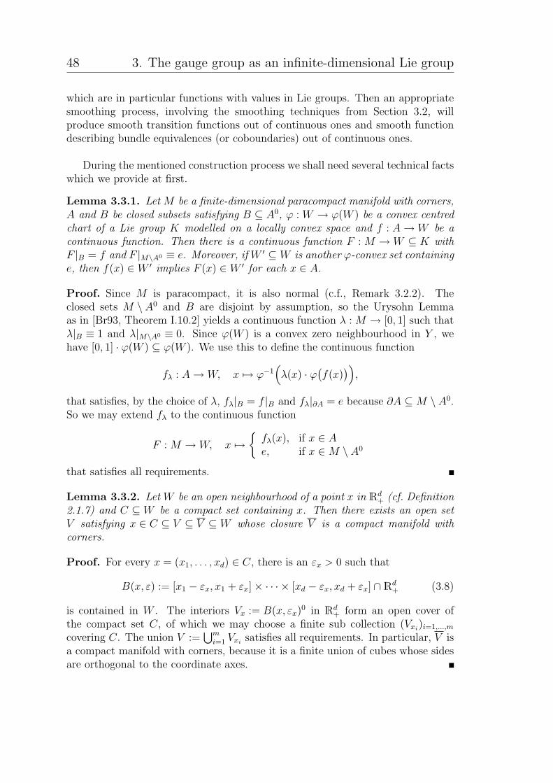
48 3. The gauge group as an infinite-dimensional Lie group
which are in particular functions with values in Lie groups. Then an appropriatesmoothing process, involving the smoothing techniques from Section 3.2, willproduce smooth transition functions out of continuous ones and smooth functiondescribing bundle equivalences (or coboundaries) out of continuous ones.
During the mentioned construction process we shall need several technical factswhich we provide at first.
Lemma 3.3.1. Let M be a finite-dimensional paracompact manifold with corners,A and B be closed subsets satisfying B ⊆ A0, ϕ : W → ϕ(W ) be a convex centredchart of a Lie group K modelled on a locally convex space and f : A→ W be acontinuous function. Then there is a continuous function F : M → W ⊆ K withF |B = f and F |M\A0 ≡ e. Moreover, if W ′ ⊆ W is another ϕ-convex set containinge, then f(x) ∈ W ′ implies F (x) ∈ W ′ for each x ∈ A.
Proof. Since M is paracompact, it is also normal (c.f., Remark 3.2.2). Theclosed sets M \ A0 and B are disjoint by assumption, so the Urysohn Lemmaas in [Br93, Theorem I.10.2] yields a continuous function λ : M → [0, 1] such thatλ|B ≡ 1 and λ|M\A0 ≡ 0. Since ϕ(W ) is a convex zero neighbourhood in Y , wehave [0, 1] · ϕ(W ) ⊆ ϕ(W ). We use this to define the continuous function
fλ : A→ W, x 7→ ϕ−1(λ(x) · ϕ
(f(x)
)),
that satisfies, by the choice of λ, fλ|B = f |B and fλ|∂A = e because ∂A ⊆M \ A0.So we may extend fλ to the continuous function
F : M → W, x 7→fλ(x), if x ∈ Ae, if x ∈M \ A0
that satisfies all requirements.
Lemma 3.3.2. Let W be an open neighbourhood of a point x in Rd+ (cf. Definition
2.1.7) and C ⊆ W be a compact set containing x. Then there exists an open setV satisfying x ∈ C ⊆ V ⊆ V ⊆ W whose closure V is a compact manifold withcorners.
Proof. For every x = (x1, . . . , xd) ∈ C, there is an εx > 0 such that
B(x, ε) := [x1 − εx, x1 + εx]× · · · × [xd − εx, xd + εx] ∩Rd+ (3.8)
is contained in W . The interiors Vx := B(x, εx)0 in Rd
+ form an open cover ofthe compact set C, of which we may choose a finite sub collection (Vxi
)i=1,...,m
covering C. The union V :=⋃mi=1 Vxi
satisfies all requirements. In particular, V isa compact manifold with corners, because it is a finite union of cubes whose sidesare orthogonal to the coordinate axes.
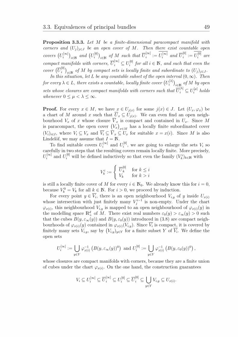
3.3. Equivalences of principal bundles 49
Proposition 3.3.3. Let M be a finite-dimensional paracompact manifold withcorners and (Uj)j∈J be an open cover of M . Then there exist countable open
covers(U
[∞]i
)i∈N and
(U
[0]i
)i∈N of M such that U
[∞]
i := U[∞]i and U
[0]
i := U[0]i are
compact manifolds with corners, U[∞]
i ⊆ U[0]i for all i ∈ N, and such that even the
cover(U
[0]
i
)i∈N of M by compact sets is locally finite and subordinate to (Uj)j∈J .
In this situation, let L be any countable subset of the open interval (0,∞). Then
for every λ ∈ L, there exists a countable, locally finite cover(U
[λ]i
)i∈N of M by open
sets whose closures are compact manifolds with corners such that U[λ]
i ⊆ U[µ]i holds
whenever 0 ≤ µ < λ ≤ ∞.
Proof. For every x ∈M , we have x ∈ Uj(x) for some j(x) ∈ J . Let (Ux, ϕx) bea chart of M around x such that Ux ⊆ Uj(x). We can even find an open neigh-bourhood Vx of x whose closure V x is compact and contained in Ux. Since Mis paracompact, the open cover
(Vx)x∈M has a locally finite subordinated cover
(Vi)i∈I , where Vi ⊆ Vx and Vi ⊆ V x ⊆ Ux for suitable x = x(i). Since M is alsoLindelof, we may assume that I = N.
To find suitable covers U[∞]i and U
[0]i , we are going to enlarge the sets Vi so
carefully in two steps that the resulting covers remain locally finite. More precisely,U
[∞]i and U
[0]i will be defined inductively so that even the family (V i
k )k∈N with
V ik :=
U
[0]
k for k ≤ iVk for k > i
is still a locally finite cover of M for every i ∈ N0. We already know this for i = 0,because V 0
k = Vk for all k ∈ N. For i > 0, we proceed by induction.
For every point y ∈ Vi, there is an open neighbourhood Vi,y of y inside Ux(i)whose intersection with just finitely many V i−1
j is non-empty. Under the chartϕx(i), this neighbourhood Vi,y is mapped to an open neighbourhood of ϕx(i)(y) inthe modelling space Rd
+ of M . There exist real numbers ε0(y) > ε∞(y) > 0 suchthat the cubes B(y, ε∞(y)) and B(y, ε0(y)) introduced in (3.8) are compact neigh-bourhoods of ϕx(i)(y) contained in ϕx(i)(Vi,y). Since Vi is compact, it is covered byfinitely many sets Vi,y, say by
(Vi,y)y∈Y for a finite subset Y of Vi. We define the
open sets
U[∞]i :=
⋃y∈Y
ϕ−1x(i)
(B(y, ε∞(y))0
)and U
[0]i :=
⋃y∈Y
ϕ−1x(i)
(B(y, ε0(y))
0),
whose closures are compact manifolds with corners, because they are a finite unionof cubes under the chart ϕx(i). On the one hand, the construction guarantees
Vi ⊆ U[∞]i ⊆ U
[∞]
i ⊆ U[0]i ⊆ U
[0]
i ⊆⋃y∈Y
Vi,y ⊆ Ux(i).
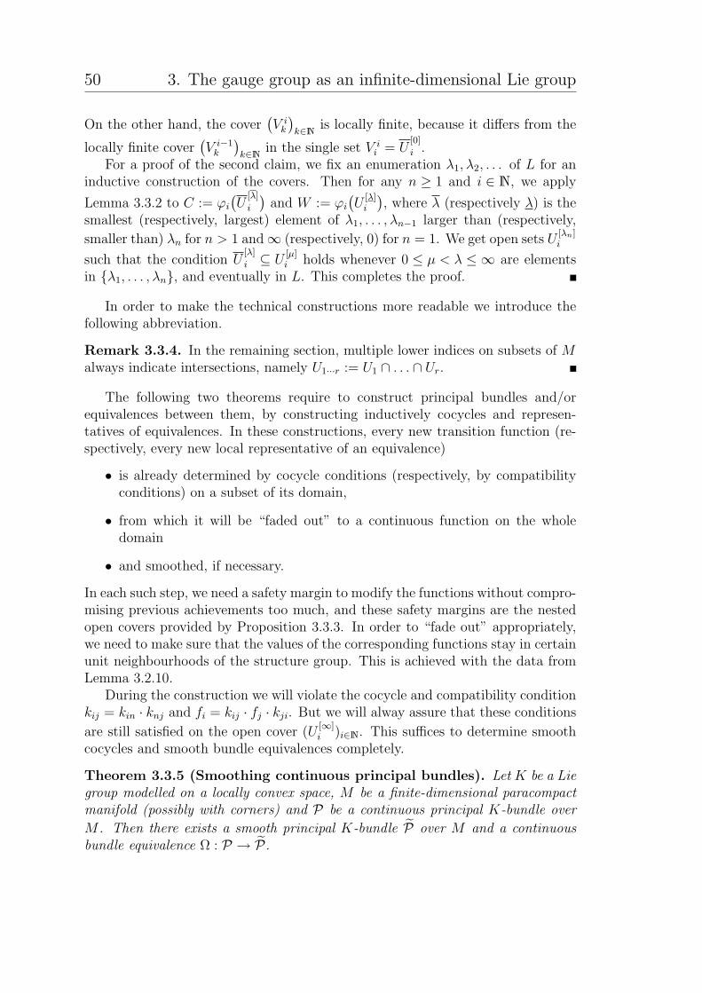
50 3. The gauge group as an infinite-dimensional Lie group
On the other hand, the cover(V ik
)k∈N is locally finite, because it differs from the
locally finite cover(V i−1k
)k∈N in the single set V i
i = U[0]
i .For a proof of the second claim, we fix an enumeration λ1, λ2, . . . of L for an
inductive construction of the covers. Then for any n ≥ 1 and i ∈ N, we apply
Lemma 3.3.2 to C := ϕi(U
[λ]
i
)and W := ϕi
(U
[λ]i
), where λ (respectively λ) is the
smallest (respectively, largest) element of λ1, . . . , λn−1 larger than (respectively,
smaller than) λn for n > 1 and∞ (respectively, 0) for n = 1. We get open sets U[λn]i
such that the condition U[λ]
i ⊆ U[µ]i holds whenever 0 ≤ µ < λ ≤ ∞ are elements
in λ1, . . . , λn, and eventually in L. This completes the proof.
In order to make the technical constructions more readable we introduce thefollowing abbreviation.
Remark 3.3.4. In the remaining section, multiple lower indices on subsets of Malways indicate intersections, namely U1···r := U1 ∩ . . . ∩ Ur.
The following two theorems require to construct principal bundles and/orequivalences between them, by constructing inductively cocycles and represen-tatives of equivalences. In these constructions, every new transition function (re-spectively, every new local representative of an equivalence)
• is already determined by cocycle conditions (respectively, by compatibilityconditions) on a subset of its domain,
• from which it will be “faded out” to a continuous function on the wholedomain
• and smoothed, if necessary.
In each such step, we need a safety margin to modify the functions without compro-mising previous achievements too much, and these safety margins are the nestedopen covers provided by Proposition 3.3.3. In order to “fade out” appropriately,we need to make sure that the values of the corresponding functions stay in certainunit neighbourhoods of the structure group. This is achieved with the data fromLemma 3.2.10.
During the construction we will violate the cocycle and compatibility conditionkij = kin · knj and fi = kij · fj · kji. But we will alway assure that these conditions
are still satisfied on the open cover (U[∞]i )i∈N. This suffices to determine smooth
cocycles and smooth bundle equivalences completely.
Theorem 3.3.5 (Smoothing continuous principal bundles). Let K be a Liegroup modelled on a locally convex space, M be a finite-dimensional paracompactmanifold (possibly with corners) and P be a continuous principal K-bundle over
M . Then there exists a smooth principal K-bundle P over M and a continuousbundle equivalence Ω : P → P.
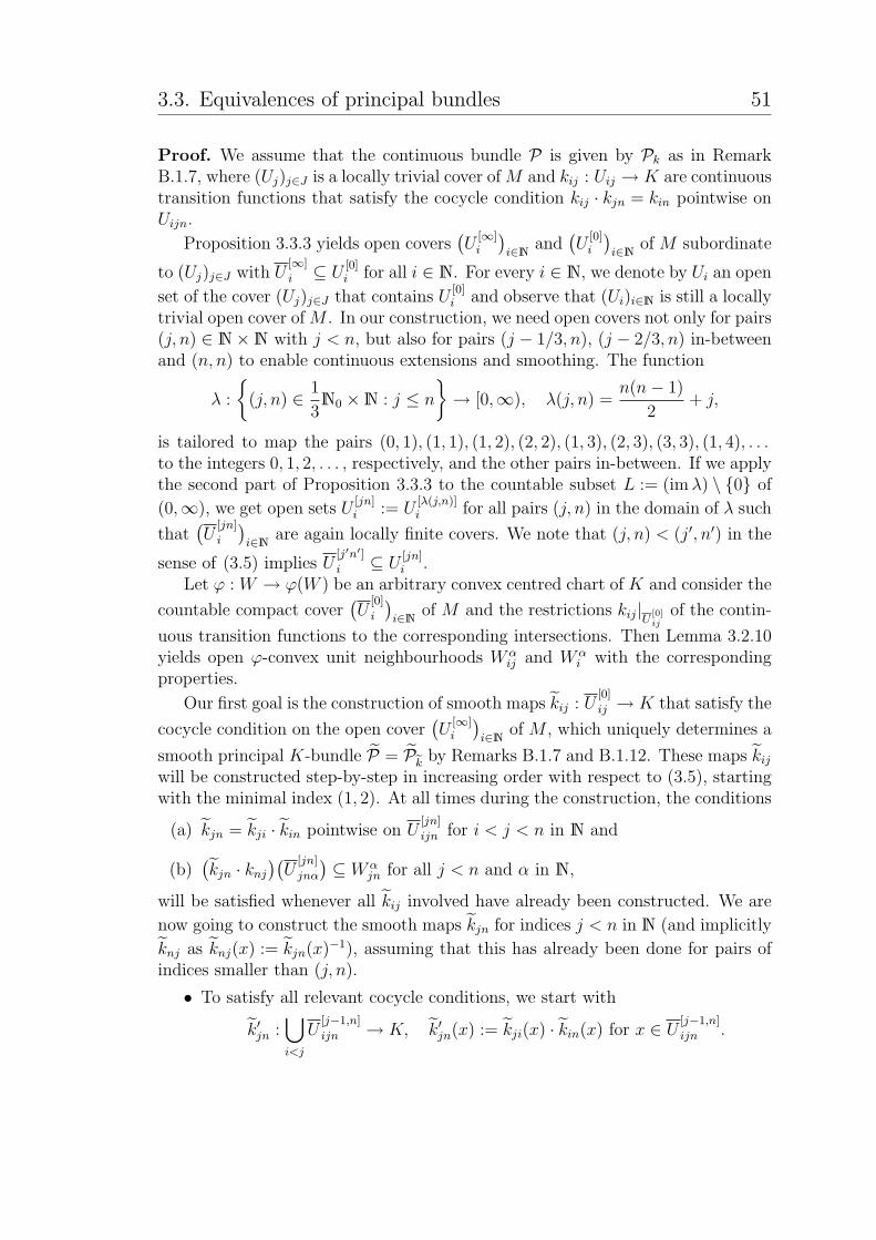
3.3. Equivalences of principal bundles 51
Proof. We assume that the continuous bundle P is given by Pk as in RemarkB.1.7, where (Uj)j∈J is a locally trivial cover ofM and kij : Uij → K are continuoustransition functions that satisfy the cocycle condition kij · kjn = kin pointwise onUijn.
Proposition 3.3.3 yields open covers(U
[∞]i
)i∈N and
(U
[0]i
)i∈N of M subordinate
to (Uj)j∈J with U[∞]
i ⊆ U[0]i for all i ∈ N. For every i ∈ N, we denote by Ui an open
set of the cover (Uj)j∈J that contains U[0]i and observe that (Ui)i∈N is still a locally
trivial open cover of M . In our construction, we need open covers not only for pairs(j, n) ∈ N×N with j < n, but also for pairs (j − 1/3, n), (j − 2/3, n) in-betweenand (n, n) to enable continuous extensions and smoothing. The function
λ :
(j, n) ∈ 1
3N0 ×N : j ≤ n
→ [0,∞), λ(j, n) =
n(n− 1)
2+ j,
is tailored to map the pairs (0, 1), (1, 1), (1, 2), (2, 2), (1, 3), (2, 3), (3, 3), (1, 4), . . .to the integers 0, 1, 2, . . . , respectively, and the other pairs in-between. If we applythe second part of Proposition 3.3.3 to the countable subset L := (imλ) \ 0 of
(0,∞), we get open sets U[jn]i := U
[λ(j,n)]i for all pairs (j, n) in the domain of λ such
that(U
[jn]
i
)i∈N are again locally finite covers. We note that (j, n) < (j′, n′) in the
sense of (3.5) implies U[j′n′]
i ⊆ U[jn]i .
Let ϕ : W → ϕ(W ) be an arbitrary convex centred chart of K and consider the
countable compact cover(U
[0]
i
)i∈N of M and the restrictions kij|U [0]
ijof the contin-
uous transition functions to the corresponding intersections. Then Lemma 3.2.10yields open ϕ-convex unit neighbourhoods W α
ij and W αi with the corresponding
properties.
Our first goal is the construction of smooth maps kij : U[0]
ij → K that satisfy the
cocycle condition on the open cover(U
[∞]i
)i∈N of M , which uniquely determines a
smooth principal K-bundle P = Pek by Remarks B.1.7 and B.1.12. These maps kijwill be constructed step-by-step in increasing order with respect to (3.5), startingwith the minimal index (1, 2). At all times during the construction, the conditions
(a) kjn = kji · kin pointwise on U[jn]
ijn for i < j < n in N and
(b)(kjn · knj
)(U
[jn]
jnα
)⊆ W α
jn for all j < n and α in N,
will be satisfied whenever all kij involved have already been constructed. We are
now going to construct the smooth maps kjn for indices j < n in N (and implicitly
knj as knj(x) := kjn(x)−1), assuming that this has already been done for pairs of
indices smaller than (j, n).
• To satisfy all relevant cocycle conditions, we start with
k′jn :⋃i<j
U[j−1,n]
ijn → K, k′jn(x) := kji(x) · kin(x) for x ∈ U [j−1,n]
ijn .
52 3. The gauge group as an infinite-dimensional Lie group
This smooth function is well-defined, because the cocycle conditions (a)for lower indices assert that for any indices i′ < i < j and any point
x ∈ U [j−1,n]
i′jn ∩ U [j−1,n]
ijn , we have
kji′(x) · ki′n(x) = kji′(x) · ki′i(x) · kii′(x) · kin(x) = kji(x) · kin(x),
because U[j−1,n]
i′ijn is contained in both U[ij]
i′ij and U[in]
i′in.
• Next, we want to extend the smooth map k′jn on⋃i<j U
[j−1,n]
ijn to a continuous
map k′jn on U[0]
jn without compromising the cocycle conditions too much. To
do this, we consider the function ϕjn := k′jnknj :⋃i<j U
[j−1,n]
ijn → K. For all
i < j, α ∈ N and x ∈ U [j−1,n]
ijnα , conditions (b) above and (3.4) of Lemma 3.2.10imply
ϕjn(x) = (k′jnknj)(x) = kji(x) ·((kij · kji)(x)︸ ︷︷ ︸
∈Wαij
)−1 · (kin · kni)(x)︸ ︷︷ ︸∈Wα
in
·kij(x)
∈ kji(x) · (W αij)
−1 ·W αin · kij(x) ⊆ W α
jn,
because U[j−1,n]
ijnα is contained in both U[ij]
ijα and U[in]
inα. Since the values ofϕjn are contained in particular in the unit neighbourhood W , we may
apply Lemma 3.3.1 to M := U[0]
jn and its subsets A :=⋃i<j U
[j−1,n]
ijn and
B :=⋃i<j U
[j−2/3,n]
ijn . It yields a continuous function Φjn : U[0]
jn → W that co-incides with ϕjn on B, is the identity outside A, and satisfies Φjn(x) ∈ W α
jn
for all x ∈ U [j−1,n]
jnα . We define k′jn : U[0]
jn → K by k′jn := Φjnkjn and note that
k′jn coincides with the smooth function k′jn on B and with kjn outside A.
• We finally get the smooth map kjn : U[0]
jn → K that we are looking for if we
apply Proposition 3.2.8 to the function k′jn on M := A := U[0]
jn, to the open
complement U of⋃i<j U
[j−1/3,n]
ijn in M , and to the neighbourhood
Ojn :=
(⋂α∈N
⌊U
[jn]
jnα,Wαjn
⌋)· kjn
of both kjn and k′jn, where k′jn ∈ Ojn follows from firstly Φjn(x) ∈ W αjn and
secondly k′jn(x) = Φjn(x) · kjn(x) ∈ W αjn · kjn(x) for all x ∈ U [jn]
jnα. Note thatOjn is really open, because Remark 3.2.3 asserts that just finitely many of the
sets U[jn]
jnα for fixed α ∈ N are non-empty and may influence the intersection.
By the choice of U , the result kjn coincides with both k′jn and k′jn on⋃i<j U
[jn]
ijn , so it satisfies the cocycle conditions (a). It also satisfies (b) bythe choice of Ojn.
3.3. Equivalences of principal bundles 53
This concludes the construction of the smooth principal K-bundle P . We use thesame covers of M and unit neighbourhoods in K for the construction of continuous
functions fi : U[0]
i → K such that
(c) fn = knj · fj · kjn pointwise on U[nn]
jn for j < n in N and
(d) fn(U
[0]
nα
)⊆ W α
n for α, n ∈ N.
Then Remark B.1.9 tells us that the restriction of the maps fi to the sets U[∞]i of
the open cover is the local description of a bundle equivalence Ω : P → P that we
are looking for. Indeed, all the sets U[nn]
jn of condition (c) contain the corresponding
sets U[∞]jn of the open cover.
We start with the constant function f1 ≡ e, which clearly satisfies condition(d). Then we construct fn for n > 1 inductively as follows:
• To satisfy condition (c), we start with
f ′n :⋃j<n
U[jn]
jn → K, f ′n(x) = knj(x) · fj(x) · kjn(x) for x ∈ U [jn]
jn .
This continuous function is well-defined, because the conditions (c) for fj on
U[jn]
j′jn ⊆ U[jj]
j′j and (a) for j′ < j < n on U[jn]
j′jn guarantee that
knj(x) · fj(x) · kjn(x) = knj(x) · kjj′(x) · fj′(x) · kj′j(x) · kjn(x)= knj′(x) · fj′(x) · kj′n(x)
holds for all x ∈ U [jn]
j′jn.
• To apply Lemma 3.3.1, we need to know something about the values of f ′n.
For arbitrary α ∈ N and x ∈ U [jn]
jnα, conditions (b), (d), and (3.3) of Lemma3.2.10 imply
f ′n(x) = knj(x) · fj(x) · kjn(x) = knj(x) ·(kjn(x) · knj(x)
)−1 · fj(x) · kjn(x)∈ knj(x) ·
(W αjn)
−1 ·W αj · kjn(x) ⊆ W α
n ,
so that the values of f ′n are, altogether, contained in the unit neighbourhood
W of K. If we apply Lemma 3.3.1 to M := U[0]
n , to f ′n on A :=⋃j<n U
[jn]
jn
and to the smaller set B :=⋃j<n U
[nn]
jn , then we get a continuous function
fn : U[0]
n → W that satisfies both (c) and (d).
This concludes the construction of the bundle equivalence.
54 3. The gauge group as an infinite-dimensional Lie group
Theorem 3.3.6 (Smoothing continuous bundle equivalences). Let K be aLie group modelled on a locally convex space, M be a finite-dimensional para-compact manifold (possibly with corners) and P and P ′ be two smooth principalK-bundles over M . If there exists a continuous bundle equivalence Ω : P → P ′,then there exists a smooth bundle equivalence Ω : P → P ′.
Proof. Let (Uj)j∈J be an open cover of M that is locally trivial for both bundles
P and P ′. Proposition 3.3.3 yields locally finite open covers(U
[λ]i
)i∈N of M for
every λ ∈ 0,∞ ∪(1 + 1
3N)
such that the closures U[λ]
i are compact manifoldwith corners and
U[∞]
i ⊆ U[j+1]i ⊆ U
[j+1]
i ⊆ U[j+2/3]i ⊆ U
[j+2/3]
i
⊆ U[j+1/3]i ⊆ U
[j+1/3]
i ⊆ U[j]i ⊆ U
[0]i ⊆ U
[0]
i ⊆ Ui
holds for all i, j ∈ N, where Ui denotes a suitable set of the cover (Uj)j∈J for everyi ∈ N. According to Remarks B.1.7 and B.1.12, we may then describe the smoothbundles P and P ′ by smooth transition functions k = (kij)i,j∈N and k′ = (k′ij)i,j∈Non the open cover (Ui)i∈N, equivalently, by their restrictions to any open cover(U
[λ]i
)i∈N from above. In these local descriptions of the bundles, the bundle equiv-
alence Ω can, as in Remark B.1.9, be seen as a family fi : Ui → K of continuousmaps for i ∈ N that satisfy
fj(x) = k′ji(x) · fi(x) · kij(x) for all i, j ∈ N and x ∈ Uij. (3.9)
We shall inductively construct smooth maps fi : U[0]
i → K such that
(a) fj = k′ji · fi · kij pointwise on U[j]
ij for all i < j in N and
(b)(fi · f−1
i
)(U
[i]
iα
)⊆ W α
i for all i, α ∈ N
are satisfied at each step, where the W αi are ϕ-convex unit neighbourhoods pro-
vided by Lemma 3.2.10 that we apply to the countable compact cover(U
[0]
i
)i∈N, to
the transition functions k′ij, and to a convex centred chart ϕ : W → ϕ(W ) of K (we
do not need the W αij in this proof). These maps fi describe a smooth bundle equiv-
alence between P and P ′ when restricted to the open cover(U
[∞]i
)i∈N, because (a)
asserts that fj = k′ji · f ′i · kij is satisfied on U[∞]ij for all i < j, in particular.
To construct the smooth function f1 : U[0]
1 → K, we apply Proposition 3.2.8 to
the continuous map f := f1 on M := A := U := U[0]
1 and to the open neighbour-hood
O1 :=⋂α∈N
⌊U
[0]
1α,Wα1
⌋· f1
3.3. Equivalences of principal bundles 55
of f1, which is indeed open, since only finitely many U[0]
1α are non-empty by Re-
mark 3.2.3. By construction, f1 satisfies (b). To construct the smooth function
fj : U[0]
j → K inductively for j > 1, we need the usual three steps:
• In order to satisfy (b) in the end, we define a continuous map
f ′j :⋃i<j
U[j−1]
ij → K, f ′j(x) := k′ji(x) · fi(x) · kij(x) for x ∈ U [j−1]
ij .
If x is an element of both U[j−1]
ij and U[j−1]
i′j for i′ < i < j, condition (a) forj − 1 and the cocycle conditions of both k and k′ assert that the so-definedvalues for f ′j(x) agree.
• This definition of f ′j, along with (3.9) and property (3.3) in Lemma 3.2.10assert that
ϕj(x) := f ′j(x) · fj(x)−1 = k′ji(x) · fi(x) · kij(x) · fj(x)−1
= k′ji(x) · fi(x) · fi(x)−1︸ ︷︷ ︸∈Wα
i
·k′ij(x) ∈ W αj
holds for all x ∈ U [j−1]
ijα , i < j and α in N. So we may apply Lemma 3.3.1 to
A :=⋃i<j U
[j−1]
ij and B :=⋃i<j U
[j−2/3]
ij to fade out ϕj to a continuous map
Φj on M := U[0]
j . Then Φj coincides with ϕi on B and maps U[j]
jα into W αj .
• Accordingly, Φj · fj is an element of the open (due to Remark 3.2.3) neigh-bourhood
Oj :=⋂α∈N
⌊U
[j]
jα,Wαj
⌋· fj
of fj and is smooth on⋃i<j U
[j−2/3]ij . If we apply Proposition 3.2.8 to
M := A := U[0]
j , U := M \⋃i<j U
[j−1/3]
ij , Oj, and to f := Φj · fj, then we ob-
tain a smooth map fj : U[0]
j → K.
The map fj satisfies (a), because so does f ′j, with which it coincides on⋃i<j U
[j]
ij .Moreover, (b) is satisfied due to the choice of Oj. This concludes the construction.
In the remaining section, we explain the relations of the preceding theoremsto classical bundle theory, non-abelian Cech cohomology and to twisted K-theory.The following lemma on smoothing homotopies will provide the tool we need whensmoothing principal bundles, which are given in terms of classifying maps.
Lemma 3.3.7. ([KM02], [Wo06, Corollary 12]) Let M be a manifold with cor-ners and N be a locally convex manifold. If f : M → N is continuous, thenthere exists a continuous map F : [0, 1]×M → N such that F (0, x) = f(x) and
56 3. The gauge group as an infinite-dimensional Lie group
F (1, ·) : M → N is smooth. Furthermore, if f, g : M → N are smooth and thereexists a continuous homotopy between f and g, then there exists a smooth homo-topy between f and g.
Lemma 3.3.8. If K is a compact Lie group, then it has a smooth universal bun-dle EK → BK with a smooth classifying space BK, which is in general infinite-dimensional.
Proof. Let Ok ⊆ GLk(R) denote the orthogonal group. If k is sufficiently large,then we may identify K with a subgroup of Ok, and from [St51, Theorem 19.6] weget the following formulae:
EK = lim→On/
(On−k × idRk
),
BK = lim→On/
(On−k ×K
).
Thus EK and BK are smooth manifolds by [Gl05, Theorem 3.1] as a direct limitof finite-dimensional manifolds. Since the action of K is smooth, it follows thatEK → BK is a smooth K-principal bundle.
Proposition 3.3.9. If P is a continuous principal K-bundle over M , K is afinite-dimensional Lie group and M is a finite-dimensional manifold with corners,then there exists a smooth principal K-bundle which is continuously equivalent toP. Moreover, two smooth principal K-bundles over M are smoothly equivalent ifand only if they are continuously equivalent.
Proof. Let C be a maximal compact subgroup of K. Since K/C is contractible,there exists a C-reduction of P , i.e., we may choose a locally trivial open cover(Ui)i∈I with transition functions kij that take values in C. They define a continuousprincipal C-bundle which is given by a classifying map f : M → BC.
By Lemma 3.3.7, f is homotopic to some smooth map f : M → BC which inturn determines a smooth principal C-bundle P overM given by smooth transitionfunctions kij. Furthermore, since f and f are homotopic, P and P are equivalent,and we thus have a continuous bundle equivalence given by continuous mappingsfi : Ui → C. The claim follows if we regard kij, kij and fi as mappings into K.
Since smooth bundles yield smooth classifying maps and smooth homotopiesof classifying maps yield smooth bundle equivalences (all the constructions in thetopological setting depend only on partitions of unity which we can assume to besmooth here), the second claim is also immediate.
We now reformulate Theorem 3.3.5 and Theorem 3.3.6 in terms of non-abelianCech cohomology.
3.3. Equivalences of principal bundles 57
Remark 3.3.10. Let M be a paracompact topological space with an open coverU = (Ui)i∈I and A be an abelian topological group. Then for n ≥ 0, an n-cochainf is a collection of continuous functions fi1...in+1 : Ui1...in+1 → A, and we denotethe set of n-cochains by Cn(U , A) and set it to 0 if n < 0. We then define theboundary operator
∂n : Cn(U , A) → Cn+1(U , A), ∂(f)i0i1...in+1 =n∑k=0
(−1)kfi0...bik...in+1,
where ik means that we omit the index ik. Then ∂n+1 ∂n = 0, and we define
Hnc (U , A) := ker(∂n)/ im(∂n−1) and Hn
c (M,A) := lim→
Hnc (U , A). (3.10)
The group H1(M,A) is the n-th continuous Cech cohomology. If, in addition,M is a smooth manifold with or without corners and A is a Lie group, thenthe same construction with smooth instead of continuous functions leads to thecorresponding n-th smooth Cech cohomology.
Remark 3.3.11. (cf. [De53, Section 12] and [GM99, 3.2.3]) If n = 0, 1, then wecan perform a similar construction as in the previous remark in the case of a notnecessarily abelian group K. The definition of an n-cochain is the same as in thecommutative case, but we run into problems when writing down the boundaryoperator ∂. However, we may define ∂0(f)ij = fi · f−1
j , ∂1(k)ijl = kij · kjl · kli and
call the elements of ∂−11 (e) 2-cocycles (or cocycles, for short).
The way to circumvent difficulties for n = 1 is the observation that even inthe non-abelian case, C1
c (U , K) acts on cocycles by fi.kij = fi · kij · f−1j . Thus we
define two cocycles kij and k′ij to be equivalent if k′ij = fi · kij · f−1j on Uij for some
fi ∈ C1(U , K), and by H1c (U , K) the equivalence classes (or the orbit space) of this
action. Then H1c (U , K) is not a group, but we may nevertheless take the direct
limitH1c (M,K) := lim
→H1c (U , K)
of sets and define it to be the 1st (non-abelian) continuous Cech cohomology of Mwith coefficients in K. By its construction, H1
c (M,K) can also be viewed as theset of equivalence classes of continuous principal K-bundles over M (cf. RemarkB.1.9).
Again, if M is a smooth manifold with corners and K is a Lie group, we canadopt this construction to define the 1st (non-abelian) smooth Cech cohomologyH1s (M,K).
Theorem 3.3.12. If M is a finite-dimensional paracompact manifold with cornersand K is a Lie group modelled on a locally convex space, then the canonical map
ι : H1s (M,K) → H1
c (M,K)
is a bijection.
58 3. The gauge group as an infinite-dimensional Lie group
Proof. We identify smooth and continuous principal bundles with Cech 1-cocyclesand smooth and continuous bundle equivalences with Cech 0-cochains as inRemark B.1.9. For each open cover U of M , we have the canonical mapH1s (U , K) → H1
c (U , K). Now each cocycle kij : Uij → K defines a principal K-bundle P with locally trivial cover U . We may assume by Theorem 3.3.5 thatP is continuously equivalent to a smooth principal bundle P , and thus that U isalso a locally trivial covering for P . This shows that the map is surjective, andthe injectivity follows from Theorem 3.3.6 in the same way. Accordingly, the mapinduced on the direct limit is a bijection.
As a special case, we now consider principal bundles, whose structure groupsis the projective unitary group of an infinite-dimensional Hilbert space H.
Remark 3.3.13. Let H be a separable infinite-dimensional Hilbert space anddenote by U(H) the group of unitary operators. If we equip U(H) with thenorm topology, then the exponential series, restricted to skew-self-adjoint opera-tors L(U(H)), induces a Banach–Lie group structure on U(H) (cf. [Mi84, Ex. 1.1]).Then U(1) ∼= Z(U(H)) and it can also be shown that PU(H) := U(H)/U(1) is aLie group modelled on L(U(H))/iR .
Remark 3.3.14. IfX is a topological space with non-trivial n-th homotopy groupπn(X) for all but one n ∈ N, then it is called an Eilenberg–MacLane spaceK(n, πn(X)). Since U(1) is a K(1,Z), the long exact homotopy sequence [Br93,Theorem VII.6.7] shows that PU(H) is aK(2,Z), since U(H) is contractible [Ku65,Theorem 3]. By the same argument, the classifying space B PU(H) is a K(3,Z),since its total space E PU(H) is contractible (cf. Corollary B.2.7). Thus
H3(M,Z) ∼= [M,B PU(H)] ∼= H1c (M,PU(H))
by [Br93, Corollary VII.13.16]. The representing class [P ] in H3(M,Z) is called theDixmier–Douady class of P (cf. [CCM98], [DD63]). It describes the obstruction ofP to be the projectivisation of an (automatically trivial) principal U(H)-bundle.
Corollary 3.3.15. If M is a paracompact manifold with corners, then
H3(M,Z) ∼= H1c (M,PU(H)) ∼= H1
s (M,PU(H)).
Bundles with PU(H) as structure group have an interesting application, be-cause they are the key-ingredient for twisted K-theory.
Example 3.3.16 (Twisted K-theory). (cf. [Ro89, Secttion 2], [BCM+02]) TheDixmier-Douady class of a principal PU(H)-bundle over M induces a twisting ofthe K-theory of M in the following manner. For any paracompact space, the K-theoryK0(M) is defined to be the Grothendieck group of the monoid of equivalenceclasses of finite-dimensional complex vector bundles over X, where addition and
3.4. The automorphism group as an infinite-dimensional Lie group59
multiplication is defined by taking direct sums and tensor products of vector bun-dles [Hu94]. Furthermore, the space of Fredholm operators Fred(H) is a represent-ing space for K-theory, i.e., K0(M) ∼= [M,Fred(H)], where [·, ·] denotes homotopyclasses of continuous maps. Since PU(H) acts (continuously) on Fred(H) by con-jugation, we can form the associated vector bundle PFred(H) := Fred(H)×PU(H) P .Then the homotopy classes of sections [M,PFred(H)] (or equivalently, the equiv-ariant homotopy classes of equivariant maps [PFred(H),Fred(H)]PU(H)) define thetwisted K-theory KP(M). Now Theorem 3.3.5 implies that we may assume P tobe smooth. Since the action of PU(H) on Fred(H) is locally given by conjugation,it is smooth, whence is PFred(H). Due to Lemma 3.3.7, we may, in the computationof KP(M), restrict our attention to smooth sections and smooth homotopies.
3.4 The automorphism group as an infinite-
dimensional Lie group
In this section we describe the Lie group structure on Aut(P) for a principalK-bundle over a compact manifold M without boundary, i.e., a closed compactmanifold. We will do this using the extension of abstract groups
Gau(P) → Aut(P)Q
−−− Diff(M)P , (3.11)
where Diff(M)P is the image of the homomorphism Q : Aut(P) → Diff(M),F 7→ FM from Definition 3.1.1. We will use this extension of abstract groupsto construct a Lie group structure on Aut(P), being induced from the Liegroup structures on Gau(P) from Section 3.1 and the classical one on Diff(M)(cf. [Le67], [Mi80], [KM97, Theorem 43.1] and [Gl06]). More precisely, we willconstruct a Lie group structure on Aut(P) that turns (3.11) into an extension ofLie groups, i.e., into a locally trivial bundle.
We shall consider bundles over bases without boundary, i.e., our base manifoldswill always be closed compact manifolds. Throughout this section we fix oneparticular given principal K-bundle P over a closed compact manifold M and wefurthermore assume that P has the property SUB.
We first clarify what we are aiming for.
Definition 3.4.1 (Extension of Lie groups). If N , G and G are Lie groups,then an extension of groups
N → G G
is called an extension of Lie groups if N is a split Lie subgroup of G. That meansthat (N, q : G→ G) is a smooth principal N -bundle, where q : G→ G ∼= G/N
is the induced quotient map. We call two extensions N → G1 G and
60 3. The gauge group as an infinite-dimensional Lie group
N → G2 G equivalent if there exists a morphism of Lie groups ψ : G1 → G2
such that the diagram
N −−−→ G1 −−−→ G
idN
y ψ
y idG
yN −−−→ G2 −−−→ G
commutes.
These extensions are treated in detail in [Ne06a], where it is shown that they are
parametrised by smooth local data arising from smooth local sections s : O → Gof q, where O ⊆ G is an open unit neighbourhood. We will not use the wholeframework from [Ne06a] rather than using the idea that we need to construct asection of Q on some unit neighbourhood of Diff(M) that has certain smoothnessproperties.
Throughout this section we have to work with trivialising systems that havesome nice properties in order to make the constructions work. This we collect inthe following remark.
Remark 3.4.2. Unless stated otherwise, for the rest of this section we choose andfix one particular smooth closed trivialising system V = (V i, σi)i=1,...,n of P suchthat
• each V i is a compact manifold with corners diffeomorphic to [0, 1]dim(M),
• V is a refinement of some smooth open trivialising system U = (Ui, τi)i=1,...,n
and we have V i ⊆ Ui and σi = τi|V i,
• each U i is a compact manifold with corners diffeomorphic to [0, 1]dim(M) andτi extends to a smooth section τi : U i → P ,
• U = (U i, τi)i=1,...,n is a refinement of some smooth open trivialising systemU ′ = (U ′
i , τj)j=1,...,m,
• the values of the transition functions kij : U ′i ∩ U ′
j → K of U ′ are contained inopen subsets Wij of K, which are diffeomorphic to open zero neighbourhoodsof k,
• P has the property SUB with respect to V (and thus with respect to U byLemma 3.1.12).
We choose V by starting with an arbitrary smooth closed trivialising systemsuch that P has the property SUB with respect to this system. Note that this existsbecause we assume throughout this section that P has the property SUB. ThenLemma B.1.8 implies that there exists a refinement U ′ = (U ′
j, τj)j=1,...,m such thatthe transition functions kij : Ui ∩ Uj → K take values in open subsets Wij of K,
3.4.The automorphism group as an infinite-dimensional Lie group 61
which are diffeomorphic to open convex zero neighbourhoods of k. Now each x ∈Mhas neighbourhoods Vx and Ux such that V x ⊆ Ux, V x and Ux are diffeomorphicto [0, 1]dim(M) and Ux ⊆ Uj(x) for some j(x) ∈ 1, . . . ,m. Then finitely manyVx1 , . . . , Vxn cover M and so do Ux1 , . . . , Uxn . Furthermore, the sections τj restrictto smooth sections on Vi, V i, Ui and Ui.
This choice of U in turn implies that kij|U i∩Ujarises as the restriction of
some smooth function on M . In fact, if ϕij : Wij → W ′ij ⊆ k is a diffeomorphism
onto a convex zero neighbourhood and fij ∈ C∞(M,R) is a smooth function withfij|U i∩Uj
≡ 1 and supp(fij) ⊆ U ′i ∩ U ′
j, then
m 7→ϕ−1ij (fij(m) · ϕij(kij(m))) if m ∈ U ′
i ∩ U ′j
ϕ−1ij (0) if m /∈ U ′
i ∩ U ′j
is a smooth function, because each m ∈ ∂(U ′i ∩ U ′
j) has a neighbourhood on which
fij vanishes, and this function coincides with kij on U i ∩ U j.Similarly, let (γ1, . . . , γn) ∈ GU(P) ⊆
∏ni=1C
∞(U i, K) be the local descriptionof some γ ∈ C∞(P,K)K . We will show that each γi|V i
arises as the restriction
of a smooth map on M . In fact, take a diffeomorphism ϕi : U i → [0, 1]dim(M).Then V i ⊆ Ui implies ϕi(V i) ⊆ (0, 1)dim(M) and thus there exits an ε > 0 suchthat ϕi(V i) ⊆ (ε, 1− ε)dim(M) for all i = 1, . . . , n. Now let
f : [0, 1]dim(M)\(ε, 1− ε)dim(M) → [ε, 1− ε]dim(M)
be a map that restricts to the identity on ∂[ε, 1− ε]dim(M) and collapses ∂[0, 1]dim(M)
to a single point x0. We then set
γ′i : M → K m 7→
γi(m) if m ∈ U i, ϕi(m) ∈ [ε, 1− ε]dim(M)
γi(ϕ−1i (f(ϕi(m)))) if m ∈ U i, ϕi(m) /∈ (ε, 1− ε)dim(M)
γi(ϕ−1i (x0)) if m /∈ Ui,
and γ′i is well-defined and continuous, because f(ϕi(m)) = ϕi(m) ifϕi(m) ∈ ∂[ε, 1− ε]dim(M) and f(ϕi(m)) = x0 if ϕi(m) ∈ ∂[0, 1]dim(M). Sinceγ′i coincides with γi on the neighbourhood ϕ−1
i ((ε, 1− ε)dim(M)), it thus is smoothon this neighbourhood. Now Proposition 3.2.8, applied to the closed set V i andthe open set M\V i yields a smooth map γi on M with γi|V i
= γi|V i.
We now give the description of a strategy for lifting special diffeomorphisms tobundle automorphisms. This should motivate the procedure of this section.
Remark 3.4.3. Let U ⊆M be open and trivialising with section σ : U → P andcorresponding kσ : π−1(U) → K, given by σ(π(p)) · kσ(p) = p. If g ∈ Diff(M) issuch that supp(g) ⊆ U , then we may define a smooth bundle automorphism g by
g(p) =
σ (g (π(p))) · k(p) if p ∈ π−1(U)p else,
62 3. The gauge group as an infinite-dimensional Lie group
because each x ∈ ∂U has a neighbourhood on which g is the identity. Furthermore,
one easily verifies Q(g) = gM = g and g−1 = g−1, where Q : Aut(P) → Diff(M) isthe homomorphism from Definition B.1.4.
The procedure is now as follows. For a suitable identity neighbourhoodO ⊆ Diff(M) we decompose g ∈ O into g1, . . . , gn such that supp(gi) ⊆ Vi. Eachgi can be lifted by the preceding remark to gi ∈ Aut(P) and then gn . . . g1 willbe the lift of g to Aut(P). In order to perform the mentioned decomposition, weneed to know some basics on the charts, turning Diff(M) into a Frechet–Lie groupmodelled on the space of vector fields V(M).
Remark 3.4.4 (Charts for Diffeomorphism Groups). Let M be a closedcompact manifold with a fixed Riemannian metric g and let π : TM →Mbe its tangent bundle and Exp : TM →M be the exponential mapping of g.Then π × Exp : TM →M ×M , Xm 7→ (m,Exp(Xm)) restricts to a diffeomor-phism on an open neighbourhood U of the zero section in TM . We setO′ := X ∈ V(M) : X(M) ⊆ U and define
ϕ−1 : O′ → C∞(M,M), ϕ−1(X)(m) = Exp(X(m))
For the following, observe that ϕ−1(X)(m) = m if and only if X(m) = 0m. Aftershrinking O′ to a convex open neighbourhood in the C1-topology, one can alsoensure that ϕ−1(X) ∈ Diff(M) for all X ∈ O′. Since π × Exp is bijective on U , ϕ−1
maps O′ bijectively to O := ϕ−1(O′) ⊆ Diff(M) and thus endows O with a smoothmanifold structure. Furthermore, it can be shown that in view of PropositionA.1.6, this chart actually defines a Lie group structure on Diff(M) (cf. [Le67],[KM97, Theorem 43.1] or [Gl06]). It is even possible to put Lie group structureson Diff(M) in the case of non-compact manifolds, possibly with corners [Mi80,Theorem 11.11], but we will not go into this generality here.
Lemma 3.4.5. For the open cover V1, . . . , Vn of the closed compact manifold Mand the open identity neighbourhood O ⊆ Diff(M) from Remark 3.4.4, there existsmooth maps
si : O → O O−1 (3.12)
for 1 ≤ i ≤ n such that supp(si(g)) ⊆ Vi and sn(g) . . . s1(g) = g.
Proof. (cf. [HT04, Proposition 1]) Let f1, . . . , fn be a partition of unity subordi-nated to the open cover V1, . . . , Vn and let ϕ : O → ϕ(O) ⊆ V(M) be the chart ofDiff(M) form Remark 3.4.4. In particular, ϕ−1(X)(m) = m if X(m) = 0m. Sinceϕ(O) is convex, we may define si : O → O O−1,
si(g) = ϕ−1((fn + . . .+ fi) · ϕ(g)
)(ϕ−1
((fn + . . .+ fi+1) · ϕ(g)
))−1
if i < n and sn(g) = ϕ−1(fn · ϕ(g)), which are smooth since they are given by apush-forward of the smooth map R× TM → TM (λ,Xm) 7→ λ ·Xm. Further-more, if fi(x) = 0, then the left and the right factor annihilate each other and thussupp(si(g)) ⊆ Vi.
3.4.The automorphism group as an infinite-dimensional Lie group 63
As mentioned above, the preceding lemma enables us now to lift elements ofO ⊆ Diff(M) to elements of Aut(P).
Definition 3.4.6. If O ⊆ Diff(M) is the open identity neighbourhood from Re-mark 3.4.4 and si : O → O O−1 are the smooth mappings from Lemma 3.4.5,then we define
S : O → Aut(P), g 7→ S(g) := gn . . . g1 , (3.13)
where gi is the bundle automorphism of P from Remark 3.4.3. This defines a localsection for the homomorphism Q : Aut(P) → Diff(M), F 7→ FM from Definition3.1.1.
We shall frequently need an explicit description of S(g) in terms of local trivi-alisations, i.e., how S(g)(σi(x)) can be expressed in terms of gj, σj and kjj′ .
Remark 3.4.7. Let x ∈ Vi ⊆M be such that x /∈ Vj for j < i and gi(x) /∈ Vjfor j > i. Then gj(x) = x for all j < i, gj(gi(x)) = gi(x) for all j > i and thusS(g)(σi(x)) = σi(gi(x)) = σi(g(x)).
In general, things are more complicated. The first gj1 in (3.13) that could moveσi(x) is the one for the minimal j1 such that x ∈ V j1 . We then have
gj1(σi(x)) = gj1(σj1(x)) · kj1i(x) = σj1(gj1(x)) · kj1i(x).
The next gj2 in (3.13) that could move gj1(σi(x)) in turn is the one for the minimalj2 > j1 such that gj1(x) ∈ V j2 , and we then have
gj2(gj1(σi(x))) = σj2(gj2 gj1(x)) · kj2j1(gj1(x)) · kj1i(x).
We eventually get
S(g)(σi(x)) = σj`(g(x)) · kj`j`−1(gj`−1
. . . gj1(x)) · . . . · kj1i(x), (3.14)
where j1, . . . , j` ⊆ 1, . . . , n is maximal such that
gjp−1 . . . gi1(x) ∈ Ujp ∩ Ujp−1 for 2 ≤ p ≤ ` and j1 < . . . < jp.
Note that we cannot write down such a formula using all j ∈ 1, . . . , n, becausethe corresponding kjj′ and σj would not be defined properly.
Of course, g and x influence the choice of j1, . . . , j`, but there exist open neigh-bourhoods Og of g and Ux of x such that we may use (3.14) as a formula forall g′ ∈ Og and x′ ∈ Ux. In fact, the action Diff(M)×M →M , g.m = g(m) issmooth ([Gl06, Proposition 7.2]), and thus in particular continuous. If
gjp . . . gj1(x) /∈ V j for 2 ≤ p ≤ ` and j /∈ j1, . . . , jp (3.15)
gjp . . . gj1(x) ∈ Ujp ∩ Ujp−1 for 2 ≤ p ≤ ` and j1 < . . . < jp (3.16)
64 3. The gauge group as an infinite-dimensional Lie group
then this is also true for g′ and x′ in some open neighbourhood of g and x. Thisyields finitely many open open neighbourhoods of g and x and we define theirintersections to be Og and Ux. Then (3.14) still holds for g′ ∈ Og and x′ ∈ Ux, be-cause (3.15) implies gj(gjp . . . gj1(x)) = gjp . . . gj1(x) and (3.16) implies thatkjpjp−1 is defined and satisfies the cocycle condition.
In order to determine a Lie group structure on Aut(P), the mapS : O → Aut(P) has to satisfy certain smoothness properties. To motivate this,assume that Aut(P) already has a smooth structure and that S : O → Aut(P) issmooth. Then the two maps
T : Gau(P)×O → Aut(P), (F, g) 7→ S(g) F S(g)−1
ω : O ×O → Aut(P), (g, g′) 7→ S(g) S(g′) S(g g′)−1
are also smooth. Moreover, for each g ∈ Diff(M)P , there exists an open identityneighbourhood Og ⊆ O such that g Og g−1 ⊆ O and that
ωg : Og → Aut(P), g′ 7→ F S(g′) F−1 S(g g′ g−1)−1
is smooth for any F ∈ Aut(P) with FM = g.Now T , ω and ωg actually take values in Gau(P) = ker(Q), because
Q : Aut(P) → Diff(M)P is a homomorphism and Q S = idO. It thus makessense to require these maps to be smooth, even if we do not jet have a smoothstructure on Aut(P). However, we will see later that requiring these maps tobe smooth determines a smooth structure on Aut(P). More generally speaking,(T, ω) is (the restriction of) a smooth factor system or locally smooth 2-cocyclefor (Gau(P),Diff(M)P) in the sense of [Ne06a]. These smooth factor systemsparametrise the set of non-abelian extensions of Diff(M)P by Gau(P) [Ne06a,Proposition II.8].
Since we can access the smooth structure on Gau(P) only via the isomorphismGau(P) ∼= C∞(P,K)K we first relate the conjugation action of Aut(P) on Gau(P)to the corresponding action of Aut(P) on C∞(P,K)K .
Remark 3.4.8. If we identify the normal subgroup Gau(P) E Aut(P) withC∞(P,K)K via
C∞(P,K)K → Gau(P), γ 7→ Fγ
with Fγ(p) = p · γ(p), then the conjugation action Aut(P)×Gau(P) → Gau(P),given by (F, Fγ) 7→ F Fγ F−1 changes into
c : Aut(P)× C∞(P,K)K → C∞(P,K)K , (F, γ) 7→ γ F−1.
In fact, this follows from
(F Fγ F−1)(p) = F(F−1(p) · γ(F−1(p))
)= p · γ(F−1(p)) = F(γF−1)(p).
3.4.The automorphism group as an infinite-dimensional Lie group 65
In the following remarks and lemmas we show the smoothness of the maps T ,ω and ωg, mentioned before.
Lemma 3.4.9. Let O ⊆ Diff(M) be the open identity neighbourhood from Remark3.4.4 and S : O → Aut(P) be the map from Definition 3.4.6. For each F ∈ Aut(P)the map C∞(P, k)K → C∞(P, k)K, η 7→ η F−1 is an automorphism of C∞(P, k)K
and the map
t : C∞(P, k)K ×O → C∞(P, k)K , (η, g) 7→ η S(g)−1
is smooth.
Proof. That η 7→ η F−1 is an element of Aut(C∞(P, k)K) follows immediatelyfrom the (pointwise) definition of the bracket on C∞(P, k)K and Lemma 2.2.24. Weshall use the isomorphism C∞(P, k)K ∼= gU ′(P) ∼= gU(P) ∼= gV(P) from Proposition3.1.4 and reduce the smoothness of t to the smoothness of
C∞(M, k)×Diff(M) → C∞(M, k), (η, g) 7→ η g−1
from Lemma 2.2.25 and to the action of g−1i on C∞(V i, k), because we have no
description of what g−1i does with Uj for j 6= i. It clearly suffices to show that the
map
ti : C∞(P, k)K ×Diff(M) → C∞(P, k)K ×Diff(M), (η, g) 7→ (η gi−1, g)
is smooth for each 1 ≤ i ≤ n, because then t = pr1 tn . . . t1 is smooth. This inturn follows from the smoothness of
C∞(U ′i , k)×Diff(M) → C∞(Ui, k), (η, g) 7→ η g−1
i
∣∣Ui, (3.17)
because this is the local description of ti. In fact, for each j 6= i there exists anopen subset V ′
j with Uj\Ui ⊆ V ′j ⊆ Uj\Vi, because V i ⊆ Ui and Uj is diffeomorphic
to (0, 1)dim(M). Furthermore, we set V ′i := Ui. Then (V ′
1 , . . . , V′n) is an open cover
of M , leading to a refinement V ′ of the trivialising system U ′ and we have
ti : gU ′(P)×O → gV ′(P), ((η1, . . . , ηn), g) 7→ (η1|V ′1 , . . . , ηi g−1i
∣∣V ′i, . . . , ηn|V ′n)
because supp(gi) ⊆ Vi and V ′j ∩ Vi = ∅ if j 6= i. To show that (3.17) is smooth,
choose some fi ∈ C∞(M,R) with fi|Ui≡ 1 and supp(fi) ⊆ U ′
i . Then
hi : C∞(U ′i , k) → C∞(M, k), η 7→
(m 7→
fi(m) · η(m) if m ∈ U ′
i
0 if m /∈ U ′i
)is smooth by Corollary 2.2.10, because η 7→ fi|U ′i · η is linear, continuous and thus
smooth. Now we have supp(gi) ⊆ Vi ⊆ Ui and thus hi(η) g−1i
∣∣Ui
= η g−1i
∣∣Ui
de-pends smoothly on g and η by Corollary 2.2.8.
66 3. The gauge group as an infinite-dimensional Lie group
The following proofs share a common idea. We will always have to show thatcertain mappings with values in C∞(P,K)K are smooth. This can be establishedby showing that their compositions with the pull-back (σi)
∗ of a section σi : V i → P(then with values in C∞(V i, K)) are smooth for all 1 ≤ i ≤ n.
As described in Remark 3.4.7, it will not be possible to write down explicitformulas for these mappings in terms of the transition functions kij for all x ∈ V i
simultaneously, but we will be able to do so on some open neighbourhood Ux of x.For different x1 and x2 these formulas will define the same mapping on Ux1 ∩ Ux2 ,because there they define (σ∗i (S(g))) = S(g) σi. By restriction and gluing we willthus be able to reconstruct the original mappings and then see that they dependsmoothly on their arguments.
Lemma 3.4.10. If O ⊆ Diff(M) is the open identity neighbourhood from Re-mark 3.4.4 and S : O → Aut(P) is the map from Definition 3.4.6, then for eachγ ∈ C∞(P,K)K the map
O 3 g 7→ γ S(g)−1 ∈ C∞(P,K)K
is smooth.
Proof. It suffices to show that γ S(g)−1 σi|V idepends smoothly on g for
1 ≤ i ≤ n. Let (γ1, . . . , γn) ∈ GU(P) ⊆∏n
i=1C∞(U i, K) be the local description
of γ. Fix g ∈ O and x ∈ V i. Then Remark 3.4.7 yields open neighbourhoods Og
of g and Ux of x (w.l.o.g. such that Ux ⊆ V i is a manifold with corners) such that
γ(S(g′)−1(σi(x′))) = γ
(σj`(g
′(x′)) ·kj`j`−1(g′j`−1
. . . g′j1(x′)) · . . . · kj1i(x′)︸ ︷︷ ︸
:=κx,g′ (x′)
)= κx,g′(x
′)−1 · γ(σj`(g
′(x′)) · κx,g′(x′) = κx,g′(x′)−1 · γj`(g′(x′)) · κx,g′(x′)︸ ︷︷ ︸
:=θx,g′ (x′)
for all g′ ∈ Og and x′ ∈ Ux. Since we will not vary i and g in the sequel, wesuppressed the dependence of κx,g′(x
′) and θx,g′(x′) on i and g. Note that each kjj′
and γi can be assumed to be defined on M (cf. Remark 3.4.2). Thus, for fixed x,the formula for θx,g′ defines a smooth function on M that depends smoothly on g′,because the action of Diff(M) on C∞(M,K) is smooth (cf. Proposition 2.2.27).
Furthermore, θx1,g′ and θx2,g′ coincide on Ux1 ∩ Ux2 , because there they bothdefine γ S(g′)−1 σi. Now finitely many Ux1 , . . . , Uxm cover V i, and since thegluing and restriction maps from Lemma 2.2.20 and Proposition 2.2.21 are smoothwe have that
γ S(g′)−1 σi = glue(θx1,g′|Ux1, . . . , θxm,g′|Uxm
)
depends smoothly on g′.
3.4.The automorphism group as an infinite-dimensional Lie group 67
The following two lemmas provide a smooth factor system (T, ω) for(Gau(P),Diff(M)P).
Lemma 3.4.11. Let O ⊆ Diff(M) be the open identity neighbourhood from Re-mark 3.4.4 and S : O → Aut(P) be the map from Definition 3.4.6. For eachF ∈ Aut(P) the map cF : C∞(P,K)K → C∞(P,K)K, γ 7→ γ F−1 is an automor-phism of C∞(P,K)K and the map
T : C∞(P,K)K ×O → C∞(P,K)K , (γ, g) 7→ γ S(g)−1 (3.18)
is smooth.
Proof. Since γ 7→ γ F−1 is a group homomorphism, it suffices to show thatit is smooth on a unit neighbourhood (Lemma A.3.3). Because the charts onC∞(P,K)K are constructed by push-forwards (cf. Proposition 3.1.8) this followsimmediately from the fact that the corresponding automorphism of C∞(P, k)K ,given by η 7→ η F−1, is continuous and thus smooth. For the same reason, Lemma3.4.9 implies that there exists a unit neighbourhood U ⊆ C∞(P,K)K such that
U ×O → C∞(P,K)K , (γ, g) 7→ γ S(g)−1
is smooth.Now for each γ0 ∈ C∞(P,K)K there exists an open neighbourhood Uγ0 such
that γ−10 · Uγ0 ⊆ U . Hence
γ S(g)−1 = (γ0 · γ−10 · γ) S(g)−1 =
(γ0 S(g)−1
)·((γ−1
0 · γ) S(g)−1),
and the first factor depends smoothly on g due to Lemma 3.4.10, and the secondfactor depends smoothly on γ and g, because γ−1
0 · γ ∈ U .
Lemma 3.4.12. If O ⊆ Diff(M) is the open identity neighbourhood from Remark3.4.4 and S : O → Aut(P) is the map from Definition 3.4.6, then
ω : O ×O → C∞(P,K)K , (g, g′) 7→ S(g) S(g′) S(g g′)−1 (3.19)
is smooth. Furthermore, if Q : Aut(P) → Diff(M), F 7→ FM is the homomorphismfrom Definition 3.1.1 then for each g ∈ Q(Diff(M)) there exists an open identityneighbourhood Og ⊆ O such that
ωg : Og → C∞(P,K)K , g′ 7→ F S(g′) F−1 S(g g′ g−1)−1 (3.20)
is smooth for any F ∈ Aut(P) with FM = g.
Proof. First observe that ω(g, g′) actually is an element ofC∞(P,K)K ∼= Gau(P) = ker(Q), because Q is a homomorphism of groups,S is a section of Q and thus
Q(ω(g, g′)) = Q(S(g)) Q(S(g′)) Q(S(g g′))−1 = idM .
68 3. The gauge group as an infinite-dimensional Lie group
To show that ω is smooth, we derive an explicit formula forω(g, g′) σi ∈ C∞(V i, K) that depends smoothly on g and g′.
Denote g := g g′ for g, g′ ∈ O and fix g, g′ ∈ O, x ∈ V i. Proceeding as inRemark 3.4.7, we find i1, . . . , i` such that
S(g)−1(σi`(x)) = σ`(g−1(x)) · ki`i`−1
((gi`−1)−1 . . . (gi1)
−1 (x)) · . . . · ki1i(x).
Accordingly we find i′`′ , . . . , i′1 for S(g′) and i′′`′′ , . . . , i
′′1 for S(g). We get as in
Remark 3.4.7 open neighbourhoods Og, Og′ of g, g′ and Ux of x (w.l.o.g. such thatUx ⊆ V i is a manifold with corners) such that for h ∈ Og, h ∈ Og′ and x′ ∈ Ux wehave S(h) · S(h′) · S(h · h′)−1(σi(x
′)) =
σi(x′) ·[ki i′′
`′′(x′)
·ki′′`′′ i
′′`′′−1
(hi′′
`′′−1 . . . hi′′1 h
−1(x′))· . . . ·ki′′1 i′`′ (h
−1(x′))
·ki′`′ i′`′−1
(h′i′
`′−1 . . . h′i′1 h
−1(x′))· . . . ·ki′1i`(h
−1(x′))
·ki`i`−1
((hi`−1
)−1 . . . (hi1 )−1(x′))· . . . ·ki1i(x′)
].
Denote by κx,h,h′(x′) ∈ K the element in brackets on the right hand side, and note
that it defines ω(h, h′) σi(x′) by Remark 3.1.2. Since we will not vary g and g′ inthe sequel we suppressed the dependence of κx,h,h′(x
′) on them.Now each kij can be assumed to be defined on M (cf. Remark 3.4.2). Thus,
for fixed x, the formula for κx,h,h′ defines a smooth function on M that dependssmoothly on h and h′, because the action of Diff(M) on C∞(M,K) is smooth(cf. Proposition 2.2.27). Furthermore, κx1,h,h′ coincides with κx2,h,h′ on Ux1 ∩ Ux2 ,because
σi(x′) · κx1,h,h′(x
′) = S(h) S(h′) S(h h′)−1(σi(x′)) = σi(x
′) · κx2,h,h′(x′)
for x′ ∈ Ux1 ∩ Ux2 . Now finitely many Ux1 , . . . , Uxm cover V i and we thus see that
ω(h, h′) σi = glue(κx1,h,h′|Ux1, . . . , κxm,h,h′|Uxm
)
depends smoothly on h and h′.To show the smoothness of ωg, we derive an explicit formula for
ωg(g′) σi ∈ C∞(V i, K). Let Og ⊆ O be an open identity neighbourhood such
that g Og g−1 ⊆ O and denote g′ = g g′ g−1 for g′ ∈ Og. Fix g′ and x ∈ V i.Proceeding as in Remark 3.4.7 we find j`, . . . , j1 such that
S(g′)−1(σi(x)) = σi`(g′−1
(x)) · kj`j`−1((gj`−1
)−1 . . . (gj1)−1
(x)) · . . . · kj1i(x).
Furthermore, let j′1 be minimal such that(F−1M S(g′)−1
M
)(x) = g−1 g′−1(x) ∈ Vj′1
3.4.The automorphism group as an infinite-dimensional Lie group 69
and let Ux be an open neighbourhood of x (w.l.o.g. such that Ux ⊆ V i is a manifold
with corners) such that g′−1
(Ux) ⊆ Vj` and g−1 g′−1(Ux) ⊆ Vj′1 . Since FM = g and
F−1(σj`(g′−1
(x′))) ∈ σj′1(g−1 g′−1(x′)) for x′ ∈ Ux
we have
F−1(σj`(g
′−1(x′))
)= σj′1(g
−1 g′−1(x′)) · kF,x,g′(x′) for x′ ∈ Ux,
for some smooth function kF,x,g′ : Ux → K. In fact, we have
kF,x,g′(x) = kσj′1(F−1(σj`(g
′−1(x)))).
After possibly shrinking Ux, a construction as in Remark 3.4.2 shows
that kσj′1F−1 σj`
∣∣∣Ux
extends to a smooth function on M . Thus
kF,x,g′|Ux∈ C∞(Ux, K) depends smoothly on g′ for fixed x.
Accordingly, we find j′2, . . . , j′`′ and a smooth function k′F,x,g′ : Ux → K (possi-
bly after shrinking Ux), depending smoothly on g such that
ωg(g′)(σi(x)) = σi(x) ·
[k′F,x,g′(x) · kj′`′j′`′−1
(g(x)) · . . . · kj′2j′1(g′−1 g−1(x)) · kF,x,g′(x)
· kj`j`−1(g′(x)) · . . . · kj1i(x)
]. (3.21)
Denote the element in brackets on the right hand side by κx,g′ . Since wewill not vary F and g in the sequel, we suppressed the dependence of κx,g′ onthem. By continuity (cf. Remark 3.4.7), we find open neighbourhoods Og′ andU ′x of g′ and x (w.l.o.g. such that U ′
x ⊆ V i is a manifold with corners) such that(3.21) defines ωg(h
′)(σi(x′)) for all h′ ∈ Og′ and x′ ∈ Ux. Then κx1,g′ = κx2,g′ on
Ux1 ∩ Ux2 , finitely many Ux1 , . . . , Uxm cover V i and since the gluing and restrictionmaps from Lemma 2.2.20 and Proposition 2.2.21 are smooth,
ωg(g′) σi = glue(κx1,g′|Ux1
, . . . , κxm,g′|Uxm)
shows that ωg(g′) σi depends smoothly on g′.
We thus have established the smoothness of the mappings T , ω and ωg. Asmentioned before, this will determine the smooth structure on Aut(P). We firstgive an description of the image of Diff(M)P := Q(Aut(P)) in terms of P , withoutreferring to Aut(P).
Remark 3.4.13. Let Q : Aut(P) → Diff(M), F 7→ FM be the homomorphismfrom Definition 3.1.1. If g ∈ Diff(M)P , then there exists an F ∈ Aut(P) thatcovers g. Hence the commutative diagram
g∗(P )gP−−−→ P
F−1
−−−→ P
g∗(π)
y π
y π
yM
g−−−→ Mg−1
−−−→ M
70 3. The gauge group as an infinite-dimensional Lie group
shows that g∗(P) is equivalent to P . On the other hand, if P ∼ g∗(P), then thecommutative diagram
P∼−−−→ g∗(P )
gP−−−→ P
π
y g∗(π)
y π
yM M
g−−−→ Mshows that there is an F ∈ Aut(P) covering g. Thus Diff(M)P consists of thosediffeomorphisms preserving the equivalence class of P under pull-backs. This showsalso that Diff(M)P is open because homotopic maps yield equivalent bundles. Itthus is contained in Diff(M)0.
Note, that it is not possible to say what Diff(M)P is in general, even in thecase of bundles over M = S1. In fact, we then have π0(Diff(S1)) ∼= Z2 (cf. [Mi84]),and the component of Diff(S1), which does not contain the identity, are preciselythe orientation reversing diffeomorphisms on S1. It follows from the description ofthe representing elements for bundles over S1 in Remark B.2.9 that pulling backthe bundle along a orientation reversing diffeomorphism inverts the representingelement in K. Thus we have g∗(Pk) ∼= Pk−1 for g /∈ Diff(S1)0. If π0(K) ∼= Z2, thenPk−1 and Pk are equivalent because [k] = [k−1] in π0(K) and thus g ∈ Diff(S1)Pk
and Diff(S1)Pk= Diff(S1). If π0(K) ∼= Z3, then Pk and Pk−1 are not equivalent
because [k] 6= [k−1] in π0(K) and thus g /∈ Diff(S1)Pkand Diff(S1)Pk
= Diff(S1)0.
Theorem 3.4.14 (Aut(P) as an extension of Diff(M)P by Gau(P)). LetP be a smooth principal K-bundle over the closed compact manifold M . If P hasthe property SUB, then Aut(P) carries a Lie group structure such that we havean extension of smooth Lie groups
Gau(P) → Aut(P)Q
−−− Diff(M)P ,
where Q : Aut(P) → Diff(M) is the homomorphism from Definition 3.1.1 andDiff(M)P is the open subgroup of Diff(M) preserving the equivalence class of Punder pull-backs.
Proof. We identify Gau(P) with C∞(P,K)K and extend S to a (possibly non-continuous) section S : Diff(M)P → Aut(P) of Q. Now the preceding lemmasshow that (T, ω) is a smooth factor system [Ne06a, Proposition II.8], which yieldsthe assertion. However, we give an explicit description of the smooth structureby applying Proposition A.1.6, for which we have to check the assumptions. Weintroduce a smooth manifold structure on W = C∞(P,K)K · S(O) by defining
ϕ : W → C∞(P,K)K ×O, F 7→(F · S(FM)−1, FM
)to be a diffeomorphism. Let O′ ⊆ O be a symmetric open identity neighbourhoodsuch that O′ ·O′ ⊆ O and for each g ∈ Diff(M) denote by Og the open identityneighbourhood from (3.20). Then multiplication in terms of ϕ is given by
(C∞(P,K)K×O′)2 3((γ, g), (γ′g′)
)7→ ϕ
(ϕ−1(γ, g)·ϕ−1(γ′, g′)
)∈ C∞(P,K)K×O,
3.4.The automorphism group as an infinite-dimensional Lie group 71
inversion in terms of ϕ is given by
C∞(P,K)K ×O 3 (γ, g) 7→ ϕ(ϕ−1(γ, g)−1) ∈ C∞(P,K)K ×O
and conjugation with F ∈ Aut(P) is given by
C∞(P,K)K ×OQ(F ) 3 (γ, g) 7→ ϕ(F · ϕ−1(γ, g) · F−1
)∈ C∞(P,K)K ×O.
Now the smoothness of these maps follows with ϕ−1(γ, g) = Fγ S(g) andQ(S(g)) = g from Lemma 3.4.9, Lemma 3.4.12 and
ϕ(ϕ−1(γ, g) · ϕ−1(γ′, g′)
)=ϕ(Fγ S(g) Fγ′ S(g′))
=(Fγ S(g) Fγ′ S(g′) S(g g′)−1, g g′
)=(Fγ S(g) Fγ′ S(g)−1︸ ︷︷ ︸
=T (γ,g)
S(g) S(g′) S(g g′)−1︸ ︷︷ ︸=ω(g,g′)
, g g′)
ϕ(ϕ−1(γ, g)−1)
=(S(g)−1 Fγ−1 S(g−1)−1, g−1
)=(S(g)−1 S(g−1)−1︸ ︷︷ ︸
=ω(g−1,g)−1
S(g−1) Fγ−1 S(g−1)−1︸ ︷︷ ︸=T (γ−1,g−1)
, g−1)
ϕ(F ϕ−1(γ, g) F−1
)=(F ϕ−1(γ, g) F−1 S(FM g F−1
M )−1, FM g F−1M
)=(F Fγ F−1︸ ︷︷ ︸
cF (γ)
F S(g) F−1 S(FM g F−1M )−1︸ ︷︷ ︸
ωFM(g)
, FM g F−1M
)Since we have a smooth section S : O → Aut(P), the quotient map
q : Aut(P) → Aut(P)/C∞(P,K)K ∼= Diff(M)P
defines the bundle projection of a smooth principal C∞(P,K)K-bundle.
Proposition 3.4.15. In the setting of the previous theorem, the natural action
Aut(P)× P → P, (F, p) 7→ F (p)
is smooth.
Proof. First we note the Gau(P) ∼= C∞(P,K)K acts smoothly on P by(γ, p) 7→ p · γ(p). Let O ⊆ Diff(M) be the open neighbourhood from Remark 3.4.4and S : O → Aut(P ), g 7→ gn . . . g1 be the map from Definition 3.4.6. ThenGau(P) S(O) is an open neighbourhood in Aut(P) and it suffices to show thatthe restriction of the action to this neighbourhood is smooth due to Lemma A.3.3.
72 3. The gauge group as an infinite-dimensional Lie group
Since Gau(P) acts smoothly on P , this in turn follows from the smoothness of themap
R : O × P → P, (g, p) 7→ S(g)(p) = gn . . . g1 (p).
In order to check the smoothness of R it suffices to check that ri : O × P → P ×O,(g, p) 7→ (gi(p), g) is smooth, because then R = pr1 rn . . . r1 is smooth. Nowthe explicit formula
gi(π(p)) =
σi(gi(π(p))) · ki(p) if p ∈ π−1(Ui)p if p ∈ π−1(V i)
c
shows that ri is smooth on(O × π−1(Ui)
)∪(O × π−1(Vi)
c)
= O × P .
Remark 3.4.16. Of course, the Lie group structure on Aut(P) from Theorem3.4.14 depends on the choice of S and thus on the choice of the chart ϕ : O → V(M)from Remark 3.4.4, the choice of the trivialising system from Remark 3.4.2 andthe choice of the partition of unity chosen in the proof of Lemma 3.4.5.
However, different choices lead to isomorphic Lie group structures on Aut(P)and, moreover to equivalent extensions. To show this we show that idAut(P) issmooth when choosing two different trivialising systems V = (V i, σi)i=1,...,n and
V ′ = (V′j, τj)j=1,...,m.
Denote by S : O → Aut(P) and S ′ : O → Aut(P) the corresponding sectionsof Q. Since
Gau(P) S(O) = Q−1(O) = Gau(P) S ′(O)
is an open unit neighbourhood and idAut(P) is an isomorphism of abstract groups,it suffices to show that the restriction of idAut(P) to Q−1(O) is smooth. Now thesmooth structure on Q−1(O) induced from S and S ′ is given by requiring
Q−1(O) 3F 7→ (F S(FM)−1, FM) ∈ Gau(P)×Diff(M)
Q−1(O) 3F 7→ (F S ′(FM)−1, FM) ∈ Gau(P)×Diff(M)
to be diffeomorphisms and we thus have to show that
O 3 g 7→ S(g) S ′(g)−1 ∈ Gau(P)
is smooth. By deriving explicit formulae for S(g) S ′(g)−1(σi(x)) on a neighbour-hood Ux of x ∈ V i, and Og of g ∈ O this follows exactly as in Lemma 3.4.12.
Remark 3.4.17. A Lie group structure on Aut(P) has been considered in[ACMM89] in the convenient setting, and the interest in Aut(P) as a symme-try group coupling the gauge symmetry of Yang-Mills theories and the Diff(M)-invariance of general relativity is emphasised. Moreover, it is also shown thatGau(P) is a split Lie subgroup of Aut(P), that
Gau(P) → Aut(P) Diff(M)P
3.4.The automorphism group as an infinite-dimensional Lie group 73
is an exact sequence of Lie groups and that the action Aut(P)× P → P is smooth.However, the Lie group structure is constructed out of quite general argumentsallowing to give the space Hom(P ,P) of bundle morphisms a smooth structureand then to consider Aut(P) as an open subset of Hom(P ,P).
The approach taken in this section is somehow different, since the Lie groupstructure on Aut(P) is constructed by foot and the construction provides explicitcharts given by charts of Gau(P) and Diff(M).
Remark 3.4.18. The approach to the Lie group structure in this section useddetailed knowledge on the chart ϕ : O → V(M) of the Lie group Diff(M) fromRemark 3.4.4. We used this when decomposing a diffeomorphism into a productof diffeomorphisms with support in some trivialising subset of M . The fact that weneeded was that for a diffeomorphism g ∈ O we have g(m) = m if the vector fieldϕ(g) vanishes in m. This should also be true for the charts on Diff(M) for compactmanifolds with corners and thus the procedure of this section should carry over tobundles over manifolds with corners.
Remark 3.4.19. In some special cases, the extensionGau(P) → Aut(P) Diff(M)P from Theorem 3.4.14 splits. This is the casefor trivial bundles and for bundles with abelian structure group K, but also forframe bundles, since we then have a natural homomorphism Diff(M) → Gau(P),g 7→ dg. However, it would be desirable to have a characterisation of the bundles,for which this extension splits.
Problem 3.4.20. Find a characterisation of those principal K-bundles P forwhich the extension Gau(P) → Aut(P) Diff(M)P splits on the group level.

Chapter 4
Calculating homotopy groups ofgauge groups
As indicated in Appendix A and Section 5.2, a good understanding of the low-dimensional homotopy groups of an infinite-dimensional Lie group is an importantkey to their Lie theory. In particular, the first and second (rational) homotopygroups are important when considering central extensions of connected Lie groups.
In this chapter we illustrate how one can access the (rational) homotopy groupsof gauge groups. Due to the weak homotopy equivalence
πn(Gau(P)) ∼= πn(Gauc(P))
from Theorem 3.2.13 we may restrict our attention to continuous gauge groups.This makes life easier since continuous functions are much more flexible thansmooth functions. The main tool will be the evaluation fibration and the resultinglong exact homotopy sequence introduced in the first section.
Of particular interest will be principal bundles over spheres and compact,closed surfaces, because they are the the easiest non-trivial examples but alreadycover many interesting cases. In particular, the case of bundles over S1 will becomeimportant in Chapter 5. Note that bundles over orientable, but non-compactor non-closed surfaces with connected structure group are always trivial (cf.Proposition B.2.10).
Throughout this chapter we will consider continuous principal bundles andidentify the continuous gauge group Gauc(P) with the space of K-equivariantcontinuous mappings C(P,K)K . To avoid confusion with the homotopygroups, we furthermore denote the bundle projection of the principal bundleP = (K, η : P →M) with η instead of π.
75
76 4. Calculating homotopy groups of gauge groups
4.1 The evaluation fibration
Let P be a continuous principal bundle. In this section we study the evaluationfibration
ev : C(P,K)K → K, γ 7→ γ(p0),
where p0 is the base-point of P . Under some mild restrictions it will turn out to bea Serre fibration and thus leads to a long exact sequence for the homotopy groupsof C(P,K)K .
Definition 4.1.1 (Evaluation fibration). If P is a continuous principal K-bundle and p0 ∈ P denotes the base-point, then the map ev : C(P,K)K → K,γ 7→ γ(p0) is called the evaluation fibration. The kernel
C∗(P,K)K := ker(ev) = γ ∈ C∞(P,K)K : γ(p0) = e
is called the pointed gauge group. Note that each γ ∈ C∗(P,K)K vanishes on thewhole fibre p0 ·K through p0, because we have γ(p0 · k) = k−1 · γ(p0) · k−1 = e.
Lemma 4.1.2. If K is a locally contractible topological group andP = (K, η : P →M) is a continuous principal K-bundle over the finite-dimensional manifold with corners M , then the evaluation fibration fromDefinition 4.1.1 defines an extension of topological groups
C∗(P,K)Kι−→ C(P,K)K
ev−−− K,
which has continuous local sections. In particular, it is a Serre fibration in thesense of [Br93, Chapter VII.6] and induces a long exact homotopy sequence
. . . . . .→ πn+1(K)δn+1−−→ πn(C∗(P,K)K)
πn(ι)−−−→ πn(C(P,K)K)
πn(ev)−−−→ πn(K)δn−→ πn−1(C∗(P,K)K) → . . . . (4.1)
Proof. If suffices to construct a continuous local section σ : W → C(P,K)K ofev for some open unit neighbourhood W ⊆ K, since then ev : C(P,K)K → Kis a locally trivial bundle and thus a locally trivial fibration (cf. [Br93, Corol-lary VII.6.12]). Since K is locally contractible, there exist open unit neighbour-hoods W,W ′ and a continuous map F : [0, 1]×W → W ′ such that F (0, k) = e,F (1, k) = k for all k ∈ W and F (t, e) = e for all t ∈ [0, 1]. For k ∈ W , we setτk := F (·, k), which is a continuous path and satisfies τk(0) = e and τk(1) = k.
Now let m0 be the base-point in M and let U ⊆M be an open neighbourhoodof m0 such that there exists a chart
ϕ : U → ϕ(U) ⊆ Rn,r+ := Rn−r ×Rr
+
4.1. The evaluation fibration 77
with ϕ(m0) = 0 and a continuous section σ : U → P with kσ : η−1(U) → K, de-termined by σ(η(p)) · kσ(p) = p. Then there exists an ε > 0 such that
Rn,r+ ∩Bε(0) := x ∈ Rn,r
+ : ‖x‖ ≤ ε ⊆ ϕ(U)
and
γk(p) =
kσ(p)
−1 · τk(1− ε−1‖ϕ(η(p))‖) · kσ(p) if p ∈ (ϕ η)−1(Bε(0))e if p /∈ (ϕ η)−1(Bε(0))
defines an element of C(P,K)K , because τk(0) = e for all k ∈ W and thus γk(p) = eif p ∈ ∂((ϕ η)−1(Bε(0))). Furthermore, τk depends continuously on k by theexponential law and so does γk. Eventually,
W 3 k 7→ γk ∈ C(P,K)K
defines a continuous section of ev.
The idea of this chapter is to consider bundles for which the homotopy groupsof the pointed gauge group πn(C∗(P,K)K) are well accessible. Then the previ-ous Lemma leads to a long exact homotopy sequence that one can use to getinformation on πn(C(P,K)K). In particular, this will turn out to be the case forbundles over spheres and compact, closed and orientable surfaces. In these cases,πn(C∗(P,K)K) can be expressed in terms of the homotopy groups πn(K) and,moreover, one can also calculate the connecting homomorphisms. To motivatethis idea we first consider the case of trivial bundles over spheres and recall somefacts on πn(K) for finite-dimensional K.
Lemma 4.1.3. If P = Sm ×K is the trivial bundle over Sm and n ≥ 1, then
πn(C(P,K)K) ∼= πn+m(K)⊕ πn(K).
Proof. For trivial bundles we have a globally defined continuous section and thusRemark 3.2.1 yields C(P,K)K ∼= C(Sm, K). Now C(Sm, K) ∼= C∗(S
m, K) oK andthus
πn(C(P,K)K) ∼= πn(C(Sm, K)) ∼= πn(C∗(Sm, K))⊕ πn(K).
Now the assertion follows from
πn(C∗(Sm, K)) ∼= π0(C∗(S
n, C∗(Sm, K)))
∼= π0(C∗(Sn ∧ Sm, K)) ∼= π0(C∗(S
n+m, K)) ∼= πn+m(K).
Remark 4.1.4. We recall some facts on the homotopy groups of a finite-dimensional Lie group K. One important fact is that π2(K) always vanishes[Mi95, Theorem 3.7]. Furthermore, we have π3(K) ∼= Z if K has a compact Liealgebra [Mi95, Theorem 3.8], because then K0 is compact [DK00, Corollary 3.6.3]and we have π3(K) = π3(K0). Furthermore, in [Mi95] one finds a table withπn(K) up to n = 15, showing in particular π4(SU2(C)) ∼= π5(SU2(C)) ∼= Z2 andπ6(SU2(C)) ∼= Z12.
78 4. Calculating homotopy groups of gauge groups
We want to reduce the determination of πn(C∗(P,K)K) to the determination ofπn(C∗(M,K)). We will first observe that we have πn(C∗(P,K)K) ∼= πn(C∗(M,K))if one considers bundles with the property that the restriction to the complementof the base-point is trivial and to functions not only vanishing in base-points butalso on a whole neighbourhood of them. This covers the cases of bundles that weare aiming for, and it will show up later that the mapping spaces are homotopicallyequivalent if the neighbourhood of the base-point is chosen appropriately.
Definition 4.1.5. If (X, x0) and (Y, y0) are pointed topological spaces andA ⊆ X, is a subset containing x0, then we denote by
CA(X, Y ) := f ∈ C(X, Y ) : f(A) = y0 ⊆ C∗(X, Y )
the space of continuous functions mapping A to the base point in Y .
Lemma 4.1.6. If P is a continuous principal K-bundle over the regular spaceX, x0 is the base point of X such that X\x0 is trivialising, then for each openneighbourhood U ⊆ X of x0 there is an isomorphism of topological groups
Cη−1(U)(P,K)K∼=−→ CU(X,K), f 7→ f σ,
where σ : X\x0 → P is a continuous section and f σ is the continuous exten-sion of f σ to X by e in x0.
Proof. Let (U1, σ1, U2σ2) be an continuous open trivialising system with U1 ⊆ U ,U2 = X\x0 and k12 : U1 ∩ U2 → K be the corresponding transition function (cf.Remark B.1.7). Then Remark 3.2.1 yields
C(P,K)K ∼= GU(P) = (γ1, γ2) ∈ C(U1, K)× C(U2, K) :
γ1(x) = k12(x) · γ2(x) · k21(x) for all x ∈ U1 ∩ U2,
where the isomorphism is given by f 7→ (f σ1, f σ2). This isomorphism in turninduces
Cη−1(U)(P,K)K ∼= GU ,U(P) := (γ1, γ2) ∈ GU(P) : γ1 ≡ e and γ2|U2∩U ≡ e,
because σ1(U1) ⊆ η−1(U) implies f(σ1(x)) = e and σ2(x) ∈ η−1(U) ⇔ x ∈ U ∩ U2.Now
CU(X,K) → GU ,U(P), f 7→ (f |U1, f |U2
) (4.2)
is an isomorphism of abstract groups which is continuous. To construct the inverseisomorphism we note that if (γ1, γ2) ∈ GU(P) and γ1 ≡ e, then we can extend γ2
to γ2 : M → K by γ2(x0) = e, because γ2 vanishes on the neighbourhood U1 of x0.Since X is assumed to be regular, there exists a closed subset C ⊆ U with x0 ∈ C,and a direct verification in the compact-open topology shows that the map
GU ,U(P) → CU(X,K), (γ1, γ2) 7→ γ2
is continuous. Since it is the inverse to (4.2), this establishes the assertion.
4.1. The evaluation fibration 79
According to the previous Lemma, we now want to replace C∗(P,K)K by ahomotopically equivalent space of gauge transformations vanishing on a suitableneighbourhood of η−1(x0). To make this precise we shall need a concept to “lo-calise” homotopy equivalences, obtained from collapsing subspaces, that becomeconstant outside some neighbourhood of the subspace. This motivates the follow-ing definition.
Definition 4.1.7. Let X be a topological space, x0 be its base-point, andU0, U1 be open neighbourhoods of x0 with U0 ⊆ U1. Then a continuous mapR : [0, 1]×X → X is called a strong retraction of U0 to x0 relative to X\U1 ifR(0, ·) = idX , R(t, U0) ⊆ U0, R(t, U1) ⊆ U1, R(1, U0) = x0 and R(t, x) = x forall t ∈ [0, 1] and x /∈ U1. This is a homotopy from the identity R(0, ·) to a mapR(1, ·), which collapses U0 to x0 and is the identity on the larger set X\U1.
Note that the previous definition is slightly different from the requirementsthat U0 is contractible and U0 → X is a cofibration. These requirements wouldonly yield the homotopy R without the requirement that R(t, ·) is the identity onsome larger set. This property will become important in the sequel, because itenables us to lift these homotopies to equivariant homotopies on the bundles.
Lemma 4.1.8. If M is a finite-dimensional manifold with corners and m0 is itsbase-point, then for each open neighbourhood V ⊆M of m0, there exist neighbour-hoods U0, U1 ⊆ V , such that there exists a strong retraction R of U0 to m0 relativeto M\U1.
In particular, if M = Sm and US, xS and xN are as in Remark B.2.9, then wecan choose U0 and U1 such that U0 = US and U1 ⊆ Sm\xN.
Proof. Let ϕ : U → ϕ(U) ⊆ Rn+ be a chart around m0 and let U0 and U1 be open
neighbourhoods of m0 in V ∩ U such that U0 ⊆ U1 and ϕ(U0) and ϕ(U1) areconvex. Furthermore, let λ : M → [0, 1] be smooth with supp(λ) ⊆ U1 and λ ≡ 1on a neighbourhood of U0. Set
R : [0, 1]×M →M, (t, x) 7→ϕ−1
((1− t · λ(x))ϕ(x) + t · λ(x) · ϕ(m0)
)if x ∈ U
x if x /∈ U.
Then supp(λ) ⊆ U1 ⊆ U1 implies that R is continuous and R(t, x) = x if x /∈ U1.Furthermore, we have R(0, ·) = idM and λ|U0
≡ 1 implies R(1, U0) = m0. Since
U0 and U1 are convex, we also have R(t, U0) ⊆ U0 and R(t, U1) ⊆ U1.
As indicated before, the group of gauge transformations, vanishing on a suitableneighbourhood of the fibre through p0, is homotopy equivalent to the pointedgauge group C∗(P,K)K . We first consider the case of trivial bundles, where wehave C(P,K)K ∼= C(M,K).
80 4. Calculating homotopy groups of gauge groups
Lemma 4.1.9. If X, Y are topological spaces, X is locally compact andR : [0, 1]×X → X is a strong retraction of U0 to x0 relative to X\U1, then theinclusion
CU0(X, Y )
ι−→ C∗(X, Y )
is a homotopy equivalence.
Proof. Since R(0, ·) = idX , we may write ι as the pull-back R(0, ·)∗. SinceR(1, ·)(U0) = x0, we get a continuous map R(1, ·)∗ : C∗(X, Y ) → CU0
(X, Y ).Since R(1, ·) is homotopic to R(0, ·), we have
R(0, ·)∗ R(1, ·)∗ ' R(0, ·)∗ R(0, ·)∗ = idC∗(X,Y ),
R(1, ·)∗ R(0, ·)∗ ' R(0, ·)∗ R(0, ·)∗ = idCU0(X,Y ),
and thus R(1, ·)∗ is a homotopy inverse to R(0, ·)∗.
Proposition 4.1.10. Let P = (K, η : P →M) be a continuous principal K-bundle over the finite-dimensional manifold with corners M , and let V be a trivi-alising open neighbourhood of the base-point m0. If R : [0, 1]×X → X is a strongretraction of U0 to m0 relative to X\U1 and U1 ⊆ V , then the inclusion
Cη−1(U0)(P,K)K → C∗(P,K)K
is is a homotopy equivalence.
Proof. Let σ : V → P be a continuous section, defining kσ : η−1(V ) → K byp = σ(η(p)) · kσ(p). Then
RP : [0, 1]× P → P, (t, p) 7→σ(R(t, η(p))) · kσ(p) if η(p) ∈ Vp if η(p) /∈ U1
is well-defined, because R(t,m) = m if m /∈ U1. Thus the map RP is continuousand RP(t, ·) is K-equivariant, because for η(p) ∈ V we have
RP(t, p · k) = σ(R(t, η(p))) · kσ(p · k) = σ(R(t, η(p))) · kσ(p) · k = RP(t, p) · k,
since kσ(p · k) = kσ(p) · k if η(p) ∈ V . Furthermore, RP(0, ·) = idP andthus the inclusion may be written as the push-forward RP(0, ·)∗. NowRP(1, η−1(U0)) ⊆ η−1(x0) and thus f(RP(1, ·)) vanishes on η−1(U0) iff ∈ C∗(P,K)K . Since
RP(1, ·)∗ RP(0, ·)∗ ' RP(0, ·)∗ RP(0, ·)∗ = idCη−1(U0)(P,K)K
andRP(0, ·)∗ RP(1, ·)∗ ' RP(0, ·)∗ RP(0, ·)∗ = idC∗(P,K)K ,
we have thatRP(1, ·)∗ is a homotopy inverse toRP(0, ·)∗ and thus that the inclusionis a homotopy equivalence.
4.1. The evaluation fibration 81
We collect the information we have so far for bundles over spheres in the fol-lowing proposition. We will throughout this section use the notation for spheresintroduced in Remark B.2.9.
Proposition 4.1.11. Let P = (K, η : P → Sm) be a continuous principal K-bundle and K be locally contractible. Then there exists a strong retraction of US
to xS relative to to Sm\U1 for some U1 ⊇ US with xN /∈ U1. Furthermore, we havethe homotopy equivalences
C∗(P,K)K ' Cη−1(US)(P,K)K ∼= CUS(Sm, K) ' C∗(S
m, K)
from Proposition 4.1.10, Lemma 4.1.6 and Lemma 4.1.9 inducing
πn(C∗(P,K)K) ∼= πn(C∗(Sm, K)) ∼= πn+m(K).
With respect to this isomorphism, the long exact homotopy sequence of the evalu-ation fibration (4.1) becomes
· · · → πn+1(K)δn+1−−→ πn+m(K) → πn(C(P,K)K) → πn(K)
δn−→ πn+m−1(K) → · · · .(4.3)
In order to perform a similar construction for bundles over compact, closed andorientable surfaces we need more information on the algebraic topology of thesesurfaces and the corresponding mapping groups.
Remark 4.1.12. Recall the notation for closed, compact and orientable surfacesfrom Remark B.2.11. The identification A2g
∼= ∂B2 shows in particular that if Xis an arbitrary topological space, then a map f : A2g → X extends to a continuousmap f : Σ → X if and only if it extends to int(B2) an thus is zero-homotopic. Thiscan be expressed by the property that π1(f) : π1(A2g) → π1(X) annihilates thecommutator (B.7) in Remark B.2.11 and hence factors through a homomorphismπ1(Σ) ∼= Z2g → π1(X).
Furthermore, if such a homomorphism π1(Σ) → π1(X) is given, then we lift it toa homomorphism π1(A2g) → π1(X), which can be represented by a map A2g → X.Since this map extends to Σ, we have shown that
C∗(Σ, X) → Hom(π1(Σ), π1(X)), f 7→ π1(f)
is surjective.Now, consider for fixed j ≤ 2g the homomorphism Z2g → Z, given on the gen-
erators by δij. If we take X = S1, then the preceding implies that we obtaincontinuous maps χj : Σ → S1 such that π1(χj)([αi]) = δij. We can even arrange χjsuch that
χj αi =
idS1 if i = j1 if i 6= j
(4.4)
82 4. Calculating homotopy groups of gauge groups
if we start with the continuous map χ0j : A2g → S1 which is on S1
j the identificationwith S1 and constantly e otherwise. Clearly, π1(χj) annihilates the commutator in(B.7) and thus extends to Σ.
Remark 4.1.13. We recall that if X is a space and A ⊆ X, then there is a bi-jection between the continuous functions on X/A and the continuous functions onX that are constant (cf. [Bo89a, §I.3.4]). For any other space Y this bijectionis given by the continuous map q∗ : C∗(X/A, Y ) → CA(X, Y ), f 7→ f q, whereq : X → X/A is the quotient map. Moreover, if A is closed, then a direct verifi-cation in the compact-open topology shows that this map is also open and thusC(X/A, Y ) and CA(X, Y ) are also homeomorphic.
In particular, if Σ is a compact, closed and orientable surface and K is atopological group, then
CA2g(Σ, K) ∼= C∗(S2, K),
and furthermore we have
πn(CA2g(Σ, K)) ∼= πn(C∗(S2, K)) ∼= πn+2(K).
We now show that these information lead to a precise description of the pointedmapping group C∗(Σ, K) in terms of C∗(S
2, K) and C∗(S1, K). Note that this
is exactly what we are aiming for, because C∗(Σ, K) is homotopy equivalent toC∗(P,K)K , and we thus obtain a precise description of C∗(P,K)K in terms of thehomotopy groups of K.
Lemma 4.1.14. Let Σ be a compact closed and orientable surface and K be atopological group and consider
r : C∗(Σ, K) → C∗(S1, K)2g, f 7→ (f α1, . . . , f α2g).
This map has CA2g(Σ, K) ∼= C∗(S2, K) as kernel, and with respect to this identifi-
cation the exact sequence
C∗(S2, K) → C∗(Σ, K)
r−− C∗(S
1, K)2g (4.5)
has a globally defined continuous (but non-homomorphic) section. In particular,C∗(Σ, K) is homeomorphic to C∗(S
2, K)× C∗(S1, K)2g .
Proof. The kernel of r is in fact CA2g(Σ, K), because f αi vanishes if and onlyif f vanishes on S1
i and A2g =⋃i S
1i . Furthermore, CA2g(Σ, K) ∼= C∗(S
2, K) byRemark 4.1.13.
A continuous inverse to r can be constructed as follows. Let χj : Σ → S1 bethe continuous maps constructed in Remark 4.1.12. Then we define
C∗(S1, K)2g → C∗(Σ, K), (f1, . . . , f2g) 7→
2g∏i=j
fj χj
4.1. The evaluation fibration 83
This is in fact a section of r, because (4.4) implies
2g∏j=1
(f χj αi)(m) = f χi αi(m) = f(m) for m ∈ S1.
Now the existence of a continuous section implies that C∗(Σ, K) is a trivial prin-cipal C∗(S
2, K)-bundle over C∗(S1, K)2g, and thus C∗(Σ, K) is isomorphic as a
C∗(S2, K)-space to C∗(S
2, K)× C∗(S1, K)2g.
For bundles over compact, closed and orientable surfaces with connected struc-ture group, the above considerations now lead to a similar long exact sequence forπn(C(P,K)K) as in the case of bundles over spheres in Proposition 4.1.11.
Proposition 4.1.15. Let P = (K, η : P →M) be a continuous principal K-bundle over a compact, closed and orientable surface Σ and let K be connectedand locally contractible. Furthermore, set UΣ := Σ\B 1
2(0) (where we identify Σ
with a quotient of B2 as in Remark B.2.11).Then there exists a strong retraction of U0 to the base-point x0 of A2g ⊆ Σ
relative to to Σ\U1 for some U0, U1 ⊆ Σ with U1 ⊆ UΣ. Furthermore, we have thehomotopy equivalences
C∗(P,K)K' Cη−1(U0)(P,K)K ∼= CU0(Σ, K) ' C∗(Σ, K) ' C∗(S
2, K)×C∗(S1, K)2g
from Proposition 4.1.10, Lemma 4.1.6, Lemma 4.1.9 and Lemma 4.1.14 inducingfor n ≥ 1
πn(C∗(P,K)K) ∼= πn(C∗(Σ, K)) ∼= πn+2(K)⊕ πn+1(K)2g.
With respect to this isomorphism, the long exact homotopy sequence of the evalu-ation fibration (4.1) becomes
· · · → πn+1(K)δn+1−−→ πn+2(K)⊕ πn+1(K)2g → πn(C(P,K)K)
→ πn(K)δn−→ πn+1(K)⊕ πn(K)2g → · · · (4.6)
The information we have so far on πn(C(P,K)K) is quite poor, since we haveno knowledge on the connecting homomorphisms δn yet. We merely get thatC(P,K)K is simply connected in the case of a principal K-bundle over S1 withsimply connected finite-dimensionalK. Thus a further treatment of the connectinghomomorphisms will be necessary in order to get more crucial information onπn(C(P,K)K).
Remark 4.1.16. A quite general theorem of Singer [Si78, Theorem 5] statesthat the weak homotopy type of C∗(P,K)K is the one of the pointed mapping group
84 4. Calculating homotopy groups of gauge groups
C∗(M,K) if M is a closed manifold of dimension of at most 4 and K = SUn(C).The method in the proof is the same that we used in this paragraph. However, ourexplicit constructions need no assumptions on the homotopy type of K and areaiming for a general treatment of gauge groups with arbitrary structure groups.So the theorem of Singer is of a different flavour.
Remark 4.1.17. Similar considerations for the pointed gauge group have beenmade in [Te05], especially for rational homotopy and rational cohomology. The ap-proach taken there focuses on bundles with simply connected semi-simple structuregroup over simply connected 4-manifolds and uses the Whitehead-Milnor Theoremto obtain an explicit description of the homotopy type of the base. In combinationwith [Si78, Theorem 5], the weak homotopy type of the pointed gauge group isreduced to the one of the pointed mapping group on the base, and this result isused to do computations in terms of mapping groups. We are aiming for moregeneral cases and thus take a more general and direct approach by using moreexplicit constructions.
Remark 4.1.18. The explicit description of πn(C∗(P,K)K) in terms of the ho-motopy groups of K in Proposition 4.1.11 and Proposition 4.1.15 is the key inour approach to the determination of the homotopy groups of the gauge groupπn(C(P,K)K). As illustrated, this works well for bundles over spheres and com-pact, closed and orientable surfaces. Furthermore, this approach extends to allclasses of bundles for which a good description of πn(C∗(M,K)) is available.
Although this will not lead to a systematic understanding of πn(C(P,K)K)without knowledge on the connecting homomorphisms, the pointed gauge group isan object of its own interest, because is acts freely on the space of connections of P[MM92, Section 6.4] and thus is often treated as the symmetry group of quantumfield theories. Furthermore, a precise knowledge of πn(C∗(P,K)K) is also desirable,because the non-vanishing of these groups can be seen as a measure for the failurefor the existing of global gauges, which is also known as the Gribov Ambiguity[MM92, Section 6.5].
Problem 4.1.19. For which manifolds M do we have a description ofπn(C∗(M,K)) in terms of the homotopy groups of K?
4.2 The connecting homomorphisms
This section is devoted to the calculation of the connecting homomorphism in theexact homotopy sequences (4.3) and (4.6) induced by the evaluation fibration.We will not solve this problem in general, but reduce it to a more familiar prob-lem in homotopy theory, i.e., the calculation of Samelson and Whitehead products.
Before starting the calculation of the connecting homomorphisms we give aconstruction principle for them.
4.2. The connecting homomorphisms 85
Remark 4.2.1. ([Br93, Theorem VII.6.7]) Let p : Y → B be a Serre fibrationwith fibre F = p−1(x0). The examples of these fibrations that we will encounterin this chapter are locally trivial bundles [Br93, Corollary VII.6.12]. The fibrationyields a long exact homotopy sequence
. . .→ πn+1(B)δn+1−−−→ πn(F )
πn(i)−−−→ πn(Y )πn(q)−−−→ πn(B)
δn−−−→ πn−1(F ) → . . .
and the construction of the connecting homomorphisms δn is as follows: Letα ∈ C∗(Bn, B) represent an element of πn(B), i.e., α|∂Bn ≡ x0. Then α can belifted to a base-point preserving map A : Bn → Y with q A = α, because q is aSerre fibration. Then A takes ∂Bn ∼= Sn−1 into q−1(x0) = A, and A|∂Bn representsδ([α]).
For bundles over compact, closed and orientable surfaces, the connecting ho-momorphism turns out to be given in terms of the connecting homomorphism forbundles S2.
Proposition 4.2.2. Let K be a connected topological group and PS2 be a contin-uous principal K-bundle over S2, represented by
b ∈ π1(K) ∼= [S2, BK]∗ ∼= Bun(S2, K).
(cf. Proposition B.2.8). Denote by δn,S2 : πn(K) → πn+1(K) the n-th connectinghomomorphism from the corresponding long exact homotopy sequence for the eval-uation fibration (4.3). Furthermore, let PΣ be a continuous principal K-bundleover the compact, closed and orientable surface Σ of genus g, represented by thesame
b ∈ π1(K) ∼= [Σ, BK]∗ ∼= Bun(Σ, K)
(cf. Proposition B.2.10). Then the n-th connecting homomorphism
δn,Σ : πn(K) → πn+1(K)⊕ πn(K)2g
from the long exact homotopy sequence for the corresponding evaluation fibration(4.6) is given by δn,Σ(a) = (δn,S2(a), 0).
Proof. Let q : Σ → B2 be the quotient map identifying A2g with the base-pointin S2 (cf. Remark B.2.11). For every principal K-bundle PS2 over S2, we have thecorresponding pull-back bundle PΣ given by
PΣQ−−−→ PS2
ηΣ
y ηS2
yΣ
q−−−→ S2
86 4. Calculating homotopy groups of gauge groups
and PΣ and PS2 have the same representing elements in π1(K)(cf. Remark B.2.12).Denote by evS2 : C(PS2 , K)K → K and by evΣ : C(PΣ, K)K → K the correspond-ing evaluation fibrations in compatible base-points of PΣ and PS2 , and observe thatevS2 = evΣ Q∗, where
Q∗ : C(PS2 , K)K → C(PΣ, K)K , f 7→ f Q
is the corresponding pull-back. This implies that if A : Bn → C(PS2 , K)K is a liftof α : Bn → K for evS2 , then Q∗ A is a lift of α for evΣ.
Now, let a ∈ πn(K) be represented by α : Bn → K with α(∂Bn) = e and letA : Bn → C(PS2 , K)K be a lift of α for evS2 . Then Q∗ A is a lift of α for evΣ,and it thus suffices to show that the restriction of the two lifts A and Q∗ A to∂Bn, taking values in C∗(PS2 , K)K and C∗(PΣ, K)K , describe the same elements inπn+1(K) ∼= πn+1(K)⊕ 0 with respect to the homotopy equivalences in Proposition4.1.11 and Proposition 4.1.15.
In order to do so, note that a section σΣ : Σ\x0 → PΣ determines uniquely asection σS2 : S2\xS → PS2 by σS2(q(x)) = Q(σΣ(x)), because q|Σ\A2g
is a home-
omorphism onto S2\xS. Thus for each y ∈ ∂Bn we have
A(y)(Q(σΣ(x))) = A(y)(σS2(q(x))),
implying
Q∗(A(y))(σΣ(x)) = A(y)(σS2(q(x))).
The homotopy equivalence from Proposition 4.1.11 and 4.1.15 replaces A|∂Bn bya mapping with values in Cη−1(U)(P,K)K for some appropriately chosen neigh-bourhood U of the corresponding base-points. Then the representative of δn,S2(a)(resp. δn,Σ(a)) is determined by pulling back A|∂Bn (resp. Q∗(A|∂Bn)) along σS2
(resp. along σΣ) and extending σ∗S2(A(y)) (resp. σ∗Σ(Q∗(A(y)))) continuously by e
for each y ∈ ∂Bn (cf. Proposition 4.1.11 and Proposition 4.1.15). Since Q∗(A(y))vanishes on η−1
Σ (q−1(U)), the continuous extension of σ∗Σ(Q∗(A(y))) vanishes onq−1(U) ⊇ A2g.
We eventually see that the πn(K)-component of δn,Σ(a) vanishes. Sincethe πn+1(K)-component is determined by identifying elements in C∗(S
2, K) withCA2g(Σ, K) via q, this also yields that the πn+1(K)-component is δS2(a).
The connecting homomorphism for bundles over spheres will be given in termsof the Samelson product, which we introduce now.
Definition 4.2.3 (Samelson Product). If K is a topological group, a ∈ πn(K)is represented by α ∈ C∗(Sn, K) and b ∈ πm(K) is represented by β ∈ C∗(Sm, K),then the commutator map
α#β : Sn × Sm → K, (x, y) 7→ α(x)β(y)α(x)−1β(y)−1
4.2. The connecting homomorphisms 87
maps Sn ∨ Sm to e. Hence it may be viewed as an element of C∗(Sn ∧ Sm, K)
and thus determines an element 〈a, b〉S := [α#β] ∈ π0(C∗(Sn+m, K)) ∼= πn+m(K).
Furthermore, it can be shown that [α#β] only depends on the homotopy classesof α and β, and we thus get a map
πn(K)× πm(K) → πn+m(K), (a, b) 7→ 〈a, b〉S
This map is bi-additive [Wh78, Theorem X.5.1] and is called the Samelson product(cf. [Wh78, Section X.5]).
As indicated before, the connecting homomorphism for bundles over spheres isgiven in terms of the Samelson product.
Theorem 4.2.4 (Connecting homomorphism is the Samelson product).If P is a continuous principal K-bundle over Sm, K is locally contractible and
b ∈ πm−1(K) ∼= [Sm, BK]∗ ∼= Bun(Sm, K)
represents P (cf. Proposition B.2.8), then the connecting homomorphisms
δn : πn(K) → πn+m−1(K)
in the long exact homotopy sequence
· · · → πn+1(K)δn+1−−→ πn+m(K) → πn(Gauc(P)) → πn(K)
δn−→ πn+m−1(K) → · · ·
from Proposition 4.1.11, induced by the evaluation fibration, is given byδn(a) = −〈b, a〉S, where 〈·, ·〉S denotes the Samelson product.
Proof. We set Bn := x ∈ Rn : ‖x‖ ≤ 1 and Sn := x ∈ Rn : ‖x‖ = 1 and usethroughout this proof the identification
([0, 1]× Sn−1)/(0 × Sn−1)∼=−→ Bn, (t, ϕ) 7→ t · ϕ (4.7)
as topological spaces without base-points. We denote by UN and US
the closed northern and southern hemispheres. Then there are sectionsσN : UN → P and σS : US → P such that the corresponding transition func-tion kP : UN ∩ US
∼= Sm−1 → K represents P (cf. Remark B.2.9). SinceUN
∼= Bm ∼= US, we may identify Gauc(P) ∼= C(P,K)K with
GU(P) := (f1, f2) ∈ C(Bm, K)2 : f1(x) = kP(x)·f2(x)·kP(x)−1 for all x ∈ ∂Bm
by the isomorphism f 7→ (f σN , f σS) (cf. Remark 3.2.1). With respect to thisidentification, the evaluation fibration is given by ev(f1, f2) = f2(0).
Each a ∈ πn(K) is represented by α : [0, 1]× Sn−1 → K withα(0, 1 × Sn−1) = e, then we may assume that α even vanishes on
88 4. Calculating homotopy groups of gauge groups
0, 1 × Sn−1 ∪ [0, 1]× x0, because Sn is homotopy equivalent to the re-duced suspension [0, 1]× Sn−1/(0, 1 × Sn−1 ∪ [0, 1]× x0). We shall constructan explicit lift of α to GU(P).
Since UN∼= Bm and α(0) = 0, we may use the identification (4.7) to define
AN : Bn × UN → K, (x, t · ϕ) 7→ k(ϕ) · α(t, x) · k(ϕ)−1 (4.8)
AS : Bn × US → K, (x, y) 7→ α(1, x) (4.9)
Then A : Bn → C(Bm, K)2, x 7→ (AN(x, ·), AS(x, ·)) defines a continuous map withvalues in GU(P), because t = 1 if t · ϕ ∈ ∂UN and thus
AN(x, t · ϕ) = k(ϕ) · α(t, x) · k(ϕ)−1 = k(ϕ) · AS(x, t · ϕ) · k(ϕ)−1.
Furthermore, A defines a lift of α, because ev(A(x)) = A2(x, 0) = α(x).Since the homotopy equivalence in Proposition 4.1.11 is given by identi-
fying US with the base-point in Sm ∼= Bm/∂Bm we thus have that δn(a) isgiven by [AN |∂Bn×Bm ] in the set of homotopy classes [∂Bn ∧ Sm, K]∗. Consider
A : Bn ×Bm → K, (x, y) 7→ AN(x, y) · α(x)−1. Then A
• vanishes on ∂Bn × ∂Bm,
• vanishes on x0 ×Bm, where x0 ∈ ∂Bn is the base-point, because α vanisheson x0 × [0, 1],
• vanishes on Bn × y0, where y0 ∈ ∂Bm is the base-point, because then t = 1and γ(ϕ) = e,
• coincides with AN on ∂Bn ×Bm, because α vanishes there,
• coincides with kP#α on Bn × ∂Bm, because then t = 1.
We take the coproduct
Sn+m−1 ∼= ∂(Bn ×Bm) = (∂Bn ×Bm) ∪ (Bn × ∂Bm) →((∂Bn×Bm)/(∂Bn×∂Bm∪x0×Bm)
)∪((Bn×∂Bm)/(∂Bn×∂Bm∪Bn×y0)
)∼= (Sn−1 ∧ Sm) ∪ (Sn ∧ Sm−1) → Sn+m−1 ∨ Sn+m−1
to define the (unique) group structure on πn+m−1(K) (cf. [Sp66, Theorem 1.6.8]).We thus have
−〈b, a〉S = −[kP#α] = −[A∣∣∣Bn×∂Bm
](∗)= [A
∣∣∣∂Bn×Bm
] = δn(a),
where (∗) follows from [Sp66, Theorem 1.6.8], because A is a continuous map on
Bn ×Bm and thus [A∣∣∣∂(Bn×Bm)
] = 0.
4.2. The connecting homomorphisms 89
As we mentioned before, there is a close interplay between the Samelson andthe Whitehead product, which we shall define now.
Definition 4.2.5. Let X be a topological space and a ∈ πn(X) and b ∈ πm(X)be represented by α ∈ C∂Bn(Bn, X) and β ∈ C∂Bm(Bm, X). We identify Sn+m−1
with ∂Bn+m = (∂Bn ×Bm) ∪ (Bm × ∂Bn) and set
(α β) : Sn+m−1 → X, (x, y) 7→α(x) if (x, y) ∈ Bn × ∂Bm
β(y) if (x, y) ∈ ∂Bn ×Bm.
Note that this is well-defined, since α(∂Bn) = ∗ = β(∂Bm). Clearly, the homo-topy class of α β depends only on the homotopy classes of α and β and thusdetermines an element 〈a, b〉WH := [α β] ∈ πn+m−1(X), and the map
πn(X)× πm(X) 3 (a, b) 7→ 〈a, b〉WH ∈ πn+m−1(X)
is called the Whitehead product (cf. [Wh78, Section X.5]).
According to [BJS60], the first appearance of the Samelson product seems tobe in [Sa53], where it occurs as an explicit formula for the Whitehead product forloop spaces, to make these products more accessible. The general relation betweenthe Samelson and the Whitehead product is the following.
Proposition 4.2.6. ([BJS60, Section 1]) If P = (K, η : P → X) is a continuousprincipal K-bundle and δn : πn(X) → πn−1(K) is the n-th connecting homomor-phism of the corresponding long exact homotopy sequence for n ≥ 1, then we have
δn+m−1(〈a, b〉WH) = 〈δn(a), δm(m)〉S (4.10)
for a ∈ πn(X) and b ∈ πm(X) and n,m ≥ 1.
Remark 4.2.7. For a continuous principal K-bundle P over Sm, the sequence
· · · → πn+1(K)δn+1−−→ πn+m(K) → πn(C∗(P,K)K) → πn(K)
δn−→ πn−1(K) → · · ·(4.11)
with the connecting homomorphisms from Theorem 4.2.4 can also be obtainedas follows. Let PK = (K, ηK : EK → BK) be a universal bundle for K, i.e., acontinuous principalK-bundle such that πn(EK) vanishes for n ∈ N0 (cf. TheoremB.2.4 and Theorem B.2.6). Furthermore, let γ : Sm → BK be a classifying mapfor P and denote by Γ : P → EK the corresponding bundle map, and denote byC(P,EK)K the space of bundle maps from P to EK.
Now each f ∈ C(P,EK)K induces a map fSm : Sm → BK, and the map
C(P,EK)KΓ 3 f 7→ fSm ∈ C(Sm, BK)γ (4.12)
90 4. Calculating homotopy groups of gauge groups
is a fibration [Go72, Proposition 3.1], where C(P,EK)KΓ (respectively C(B,BK)γ)denotes the connected component of Γ (respectively γ), and we have a homeomor-phism
F = f ∈ C(P,EK)KΓ : fSm = γ ∼= C(P,K)K
[Go72, Proposition 4.3]. Since πn(C(P,EK)KΓ ) vanishes [Go72, Theorem 5.2], thelong exact homotopy sequence of the fibration (4.12) leads to
πn−1(C(P,K)KΓ ) ∼= πn(C(Sm, BK)γ)
(cf. [Ts85, Theorem 1.5] and [AB83, Proposition 2.4]). We now consider the evalu-ation fibration ev : C(Sm, BK)γ → BK, f 7→ f(xS). This map is in fact a fibration[Br93, Theorem VII.6.13] with fibre ev−1(xS) =: C∗(S
m, BK)γ, and we thus get along exact homotopy sequence
. . .→ πn+1(BK)δn+1−−→ πn(C∗(S
m, BK)γ) → πn(C(Sm, BK)γ)
→ πn(BK)δn−→ πn−1(C∗(S
m, BK)γ) → . . . . (4.13)
If we identify πn(C∗(Sm, BK)γ) with πn+m(BK) (cf. [Wh46, 2.10]), then the con-
necting homomorphism in this sequence is given by δn+1(a) = −〈a, b〉WH , whereb = [γ] ∈ πm(BK) and 〈·, ·〉WH denotes the Whitehead product (cf. [Wh46, Theo-rem 3.2] and [Wh53, 3.1]).
Since πn(EK) vanishes, each connecting homomorphismδn : πn(BK) → πn−1(K) from the long exact homotopy sequence for PK isan isomorphism, and with respect to this identification, the exact sequence from(4.13) becomes (4.11). Since, under this identification, the Whitehead productbecomes the Samelson product (cf. (4.10)), the connecting homomorphism is thengiven by the Samelson product as in Theorem 4.2.4.
Remark 4.2.8. For bundles over spheres and over compact closed and orientablesurfaces the connecting homomorphisms are given in terms of the Samelson or theWhitehead product. In the case of bundles over surfaces, the reduction of theconnecting homomorphisms to the ones for bundles over spheres relies on the factthat these bundles arise from clutching two trivial bundles over a closed 2-cell andthe complement of its interior together along a single characteristic map. Nowthis construction produces more general bundles over more general manifolds (i.e.,simply-connected 4-manifolds by the Milnor-Whitehead Theorem, cf. [Te05]), andshould lead to more systematic information on πn(C(P,K)K).
Problem 4.2.9. Find more explicit descriptions of principal bundles arising assimply clutched bundles, i.e., as bundles over manifolds of dimension n, whosebases possess a trivialising cover consisting of a closed n-cell and the complementof its interior.
4.3. Formulae for the homotopy groups 91
4.3 Formulae for the homotopy groups
In this section we describe how known results on the Samelson and White-head products lead to explicit formulae for the (rational) homotopy groupsof the gauge group. This depends on the amount of known results for theseproducts. We are mainly interested in the low-dimensional homotopy groups(i.e., π1(C(P,K)K) and π2(C(P,K)K)), which causes some problems, becausethese products are mostly considered in higher dimensions (cf. [Bo60]). However,at least for some examples and in the rational case, these products are well-known.
One example, in which we can use the results of the previous section is thequaterionic Hopf fibration.
Example 4.3.1 (The quaterionic Hopf fibration). Consider the quaternionskew-field H ∼= R4 with the euclidean norm
√q1q1 + . . .+ qnqn = ‖q‖ on Hn ∼= R4n
andS4n−1 := q ∈ Hn : ‖q‖ = 1.
Furthermore, consider the projective spaces PHn−1 := Hn/ ∼ withq ∼ q′ :⇔ q = λq′ for some λ ∈ S3. Then S3 ∼= SU2(C) acts on S4n−1 by(q1, . . . , qn) · k = (q1k, . . . , qnk), and the orbit map composed with the quotientmap yields a surjection η′ : S4n−1 → PHn−1. This defines a continuous principalSU2(C)-bundle (SU2(C), η′ : S4n−1 → PHn−1), provided by the trivialisations
η′−1(Uk) 3 (q1, . . . , qn) 7→ [(q1, . . . , qn)], |qk|−1qk ∈ Uk × SU2(C),
where Uk := [q] ∈ PHn−1 : qk 6= 0. Now PH1 ∼= S4, since both spaces are home-omorphic to the one-point compactification of H, and thus we get a continuousprincipal SU2(C)-bundle H := (SU2(C), η : S7 → S4), called the quaterionic Hopffibration.
A characteristic map (cf. Remark B.2.9) γ : SU2(C) → SU2(C) for this bundlecan obtained as follows. We view S4 as the quotient of q ∈ H : ‖q‖ ≤ 1 by itsboundary. Then the homeomorphism from S4 to the one-point compactification ofH is given by
ϕ : S4 → H ∪ ∞, q 7→ q
1−‖q‖ if ‖q‖ < 1
∞ if ‖q‖ = 1.
Composing ϕ|‖q‖<1 with the section
σ′ : H→ S7, q 7→ 1
‖(1, q)‖(1, q)
yields a map σ, which we may continuously extend to ‖q‖ = 1 by settingσ(q) = (0, q) in this case. This results in a map σ satisfying η σ = q, whereq is the quotient map defining S4. We thus may take γ = idSU2(C) as the maprepresenting the equivalence class of H.
92 4. Calculating homotopy groups of gauge groups
More generally, principal SU2(C)-bundles over S4 are classified by their socalled Chern number k ∈ Z ∼= π3(SU2(C)) (cf. [Na97, Theorem 6.4.2]), and thequaterionic Hopf fibration has Chern number 1. We denote by Pk the principalSU2(C)-bundle over S4 with Chern number k.
As mentioned before, the crucial Samelson product in this example is well-known and now leads to an explicit description of π1(C(P,K)K) and π2(C(P,K)K)for SU2(C)-bundles over S4.
Proposition 4.3.2. If Pk is a principal SU2(C)-bundle over S4 of Chern numberk ∈ Z, then π1(C(Pk, K)K) ∼= Z2 and π2(C(Pk, K)K) ∼= Zgcd(k,12). In particular, ifP1 denotes the quaterionic Hopf fibration, then π2(C(P1, K)K) vanishes.
Proof. (cf. [Ko91, Lemma 1.3]) Recall the homotopy groups of SU2(C) from Re-mark 4.1.4. First we note that we have π1(C(P,K)K) ∼= Z2 by the exact sequence
π2(SU2(C))︸ ︷︷ ︸=0
→ π5(SU2(C))︸ ︷︷ ︸∼=Z2
→ π1(C(Pk, K)K) → π1(SU2(C))︸ ︷︷ ︸=0
from Proposition 4.1.11. Since Pk is classified by the Chern numberk ∈ Z ∼= π3(SU2(C)), Theorem 4.2.4 provides an exact sequence
π3(SU2(C))δk2−→ π6(SU2(C))
π2(i)−−→ π2(C(Pk, K)K) → π2(SU2(C)),
where δk2 : π3(SU2(C)) → π6(SU2(C)) is given by a 7→ −〈k, a〉S. Sinceπ3(SU2(C)) ∼= Z, π6(SU2(C)) ∼= Z12 and 〈1, 1〉S generates π6(SU2(C)) [Pu04,Corollary 6.2], we may assume that δk2 : Z→ Z12 is the map Z 3 z 7→ −[kz] ∈ Z12
due to the bi-additivity of 〈·, ·〉S. Since π2(SU2(C)) is trivial, we have that π2(i)is surjective and
im(π2(i)) ∼= Z12/ ker(π2(i)) = Z12/ im(δk2) = Z12/(kZ12) ∼= Zgcd(k,12).
Systematical results on the Samelson product in low dimensions seem not tobe available in the literature. This is different for the rational Samelson products,which we will consider now.
Remark 4.3.3. As explained in Section A.2, in infinite-dimensional Lie the-ory one often considers (period-) homomorphisms ϕ : πn(G) → V for an infinite-dimensional Lie group G and an R-vector space V , which we consider here as aQ-vector space. If n ≥ 1, then πn(G) is abelian and this homomorphism factorsthrough the canonical map ψ : πn(G) → πn(G)⊗Q, a 7→ a⊗ 1, and
ϕ : πn(G)⊗Q→ V, a⊗ x 7→ x ϕ(a).
It thus suffices for many interesting questions arising from infinite-dimensional Lietheory to consider the rational homotopy groups πQn (G) := πn(G)⊗Q for n ≥ 1.
Furthermore, the functor ⊗Q in the category of abelian groups, sending A toAQ := A⊗Q and ϕ : A→ B to ϕQ := ϕ⊗ idQ : A⊗Q→ B ⊗Q, preserves exactsequences, since Q is torsion free and hence flat (cf. [Br93, Section V.6]).
4.3. Formulae for the homotopy groups 93
Lemma 4.3.4. If K is a finite-dimensional Lie group and n,m ≥ 1, then therational Samelson product
〈·, ·〉QS : πQn (K)× πQm(K) → πQn+m(K), a⊗ x, b⊗ y 7→ 〈a, b〉S ⊗ xy
vanishes.
Proof. We first consider the case where K is connected. If a ∈ πn(K) andb ∈ πm(K), then 〈a, b〉S is an element of the torsion subgroup of πn+m(K) [Ja59],and the assertion follows from the fact that tensoring with Q kills the torsionsubgroup.
If K is not connected, then a ∈ πn(K) ∼= πn(K0) is represented by a mapα : Sn → K0 and b ∈ πm(K) is represented by a map β : Sm → K0, because Sn
and Sm are arcwise connected for n,m ≥ 1. Then α#β (cf. Definition 4.2.3) alsotakes values in K0, as well as (α#β)` for each ` ∈ N. Now 〈[α], [β], 〉S is a torsionelement if and only if there exists an integer `0 such that (α#β)`0 is null-homotopic,i.e., extends to Bm+n+1. Thus `0〈[α], [β]〉 = 0, for [α] ∈ πn(K0) and β ∈ πm(K0)if and only if `0〈[α], [β]〉 = 0, for [α] ∈ πn(K) and β ∈ πm(K), and the assertionfollows from the case where K is connected.
Theorem 4.3.5 (Rational homotopy groups of gauge groups). Let K be afinite-dimensional Lie group and P be a continuous principal K-bundle over X,and let Σ be a compact orientable surface of genus g. If X = Sm, then
πQn (Gauc(P)) ∼= πQn+m(K)⊕ πQn (K)
for n ≥ 1. If X = Σ and K is connected, then
πQn (Gauc(P)) ∼= πQn+2(K)⊕ πQn+1(K)2g ⊕ πQn (K)
for n ≥ 1.
Proof. First note, that in the case on a non-closed surface each bundle withconnected structure group is trivial (Proposition B.2.10), which yields the assertionin this case. In the other cases, we obtain with Remark 4.3.3 an exact rationalhomotopy sequence from the exact sequence for the evaluation fibration (4.3) fromProposition 4.1.11 and (4.6) from Proposition 4.1.15. Then the preceding lemmaimplies that the connecting homomorphisms in these sequences vanish, because theconnecting homomorphisms for the homotopy sequences are given in terms of theSamelson product by Proposition 4.2.2 and Theorem 4.2.4. Thus the long exactrational sequence splits into short ones. Furthermore, these short exact sequencessplit linearly, since each of them involves vector spaces.
Remark 4.3.6. The rational homotopy groups of finite-dimensional Lie groupsare those of products of odd-dimensional spheres [FHT01, Section 15.f], which
94 4. Calculating homotopy groups of gauge groups
are well known [FHT01, Example 15.d.1]. Thus Theorem 4.3.5 gives a detaileddescription of the rational homotopy groups for the gauge group of bundles overspheres and compact, closed and orientable surfaces.
Although this knowledge is sufficient for many questions in infinite-dimensionalLie theory, it would be desirable to have more explicit descriptions of πn(C(P,K)K)for larger classes of bundles. As illustrated in Proposition 4.3.2, a detailed knowl-edge of Samelson- and Whitehead Products would lead to more of these descrip-tions but this knowledge is not available in low dimensions.
Problem 4.3.7. Which explicit formulae for the Samelson- or Whitehead productlead to more explicit descriptions of πn(C(P,K)K) for larger classes of bundles?
Chapter 5
Central extensions of gaugegroups
In this chapter we construct a central extension of the identity component Gau(P)0
of the gauge group and an action of the automorphism group Aut(P) on it. Theprocedure is motivated by ideas from [PS86], [LMNS95] and [MN03].
The general idea for constructing central extensions of infinite-dimensional Liegroups is to construct central extensions of the corresponding Lie algebras andthen check whether they are induced by corresponding central extensions of theirgroups. The tools we use here are provided in [Ne02a].
We shall consider bundles over bases without boundary, i.e., our base manifoldswill always be closed compact manifolds. Throughout this section we fix oneparticular given smooth principal K-bundle P over a closed compact manifold M .We furthermore assume K to be locally exponential. This ensures, in particular,that all bundles occurring in this section have the property SUB with respect toeach smooth closed trivialising system (cf. Lemma 3.1.13).
5.1 A central extension of the gauge algebra
The first step is to construct central extensions of the gauge algebra. In the caseof trivial bundles we have gau(P) ∼= C∞(M, k) and from [MN03] the cocycle
C∞(M, k)× C∞(M, k) 3 (η, µ) 7→ [κ(η, dµ)] ∈ Ω1(M,Y )/dC∞(M,Y ), (5.1)
where κ : k× k → Y is a continuous, symmetric, k-invariant bilinear map. In thissection we shall illustrate how this cocycle generalises to arbitrary smooth bundlesby replacing the ordinary differential with a covariant derivative (cf. [LMNS95]).
We first introduce the notation we use throughout this chapter.
95
96 5. Central extensions of gauge groups
Definition 5.1.1. If P is a smooth principal K-bundle and Ad(P) is its adjointbundle, then we have the isomorphisms
gau(P) ∼= C∞(P, k)K ∼= S(ad(P)) = Ω0(M, ad(P))
from Proposition 3.1.4. Let Y be a locally convex space, and consider the trivialaction λ : K × Y → Y . Then the associated bundle λ(P) is trivial, and we thushave Ω1(M,λ(P)) ∼= Ω1(M,Y ). If κ : k× k → Y is a continuous K-invariant bilin-ear form, then it is in particular K-equivariant with respect to Ad and λ, and weget from Lemma B.3.11 a continuous linear map
κ∗ : gau(P)× Ω1bas(P, k)
K → Ω1(M,Y ),
when identifying gau(P) with Ω0(M,Ad(P)) and Ω1bas(P, k)
K with Ω1(M,Ad(P))as in Remark B.3.5 and Ω1(M,λ(P)) with Ω1(M,Y ).
Remark 5.1.2. If M is a closed finite-dimensional manifold and Y is a Frechetspace, then we define
zM(Y ) := Ω1(M,Y )/dC∞(M,Y ).
Since dC∞(M,Y ) is the annihilator of the continuous linear maps
λα : Ω1(M,Y ) → Y, ω 7→∫S1
α∗ω, (5.2)
for α ∈ C∞(S1,M), it follows that dC∞(M,Y ) is in particular closed in Ω1(M,Y )so that we obtain a locally convex Hausdorff vector topology on zM(Y ). Fur-thermore, since zM(Y ) is a quotient of the Frechet space Ω1(M,Y ) by the closedsubspace dC∞(M,Y ), it is again a Frechet space. Note that Y is in particularsequentially complete, ensuring the existence of the integral in (5.2).
As indicated before, we substitute the ordinary differential in (5.1) by a covari-ant derivative to obtain the cocycle describing the central extension of gau(P).
Lemma 5.1.3. Let P be a smooth principal K-bundle over the closed finite-dimensional manifold M , A ∈ Ω1(P, k) be a connection 1-form and
dA : gau(P) → Ω1bas(P,Ad(P))K .
be the induced covariant derivative from Lemma B.3.7. If Y is a locally convexspace and κ : k× k → Y is continuous, bilinear, symmetric and K-invariant, then
ωκ,A : gau(P)× gau(P) → zM(Y ), (η, µ) 7→[κ∗(η, d
A µ)]
(5.3)
is a continuous cocycle on gau(P).
5.1. A central extension of the gauge algebra 97
Furthermore, if A,A′ ∈ Ω1(P, k) are two connection 1-forms of P, thenωκ,A − ωκ,A′ is a coboundary, i.e., there exists a continuous linear mapλ : gau(P) → zM(Y ) such that we have
ωκ,A(η, µ)− ωκ,A′(η, µ) = λ([η, µ]) (5.4)
for η, µ ∈ gau(P).
Proof. The continuity follows directly from Lemma B.3.11, because ωκ,A isthen only a composition of continuous maps. Let EY be the trivial vectorbundle M × Y over M . With the identifications Ω0(M, EY ) ∼= C∞(M,Y ) andΩ1(M, EY ) ∼= Ω1(M,Y ), the covariant derivative on EY induced from A is f 7→ df(cf. Lemma B.3.7).
That ωκ,A is alternating, i.e., ωκ,A(η, µ) = −ωκ,A(µ, η) follows with LemmaB.3.13 from
dκ∗(η, µ) = κ∗(dA η, µ) + κ∗(η, d
A µ) = κ∗(µ, dA η) + κ∗(η, d
A µ)
The cocycle condition is
κ∗([η, µ], dA ν) + κ∗([ν, η], dA µ) + κ∗([µ, ν], d
A η) ∈ dC∞(M,Y )
for all η, µ, ν ∈ gau(P). With Lemma B.3.13, we get
dκ∗([η, µ], ν) = κ∗(dA [η, µ], ν)+κ∗([η, µ], dA ν) = κ∗([d
A η, µ], ν)+κ∗([η, dA µ], ν)
+ κ∗([η, µ], dA ν) = κ∗([µ, ν], dA η) + κ∗([ν, η], d
A µ) + κ∗([η, µ], dA ν),
because κ is K-invariant and thus κ([x, y], z) = κ(x, [y, z]) for all x, y, z ∈ k.To show that ωκ,A − ωκ,A′ is a coboundary, we observe that we get from Lemma
B.3.7 dA µ− dA′µ = [A′ − A, µ], and thus
ωκ,A(η, µ)− ωκ,A′(η, µ) = κ∗(η, [A′ − A, µ]) = κ∗(A− A′, [η, µ]).
Hence λ : gau(P) → zM(Y ), ν 7→ [κ∗(A− A′, ν)] satisfies (5.4).
Definition 5.1.4. The continuous cocycle ωκ,A from the preceding lemma is calledcovariant cocycle.
Remark 5.1.5. Lemma 5.1.3 implies that the class [ωκ,A] ∈ H2c (gau(P), zM(Y ))
is independent of the choice of the connection 1-form A. Thus, the equivalenceclass of the central extension
gau(P)ωκ,A= zM(Y )⊕ωκ,A
gau(P) with [(x, η), (y, µ)] = (ωκ,A(η, µ), [η, µ])
(cf. Remark A.2.2) does not depend on the choice of A but only on the bundle Pand on κ.
98 5. Central extensions of gauge groups
Now the question arises how exhaustive the constructed central extension ofgau(P) is, i.e., for which spaces it is universal.
Remark 5.1.6. It has been shown in [Ma02] that the central extension of gau(P)from Remark 5.1.5 is universal in the case of a trivial bundle, finite-dimensionaland semisimple k and the universal invariant bilinear form k× k → V (k), since thengau(P) ∼= C∞(M, k) and the cocycle (5.1) is universal.
For non-trivial bundles it is not know to the author whether the central exten-sion of the gauge algebra is universal. The arguments from [Ma02] do not carryover directly, because they use heavily the fact that k embeds as a subalgebra intoC∞(M, k). This is not true for C∞(P, k)K and causes the main problem.
Problem 5.1.7. For which bundles (beside trivial ones) and for which locallyconvex spaces is the central extension of Remark 5.1.5 universal?
5.2 Integrating the central extension of the
gauge algebra
In this and the following section we check the integrability condition for the central
extension of gau(P) from Remark 5.1.5. The background on central extensions ofLie groups, Lie algebras and their relation is provided in Section A.2.
Unless stated otherwise, throughout this section, we fix one smooth principalK-bundle P over M for a locally exponential Lie group K and a closed compactmanifold M . Furthermore, κ : k× k → Y is always a continuous, symmetric andK-invariant bilinear form and a cocycle ωκ,A representing [ωκ,A] from Remark 5.1.5for an arbitrary connection 1-form A as in Lemma 5.1.3.
Note that we are not assuming K to be connected, because this would causeprincipal bundles over S1 to become trivial and thus would exclude twisted affineKac–Moody groups. To this particular class of examples we turn in Section 5.4.
We first motivate the procedure in this section by collecting some results from[Ne02a] and [MN03]. The most important thing that we will have to consider isthe period homomorphism associated to a continuous cocycle.
Definition 5.2.1. Let G be a connected Lie group. Then [Ne02a, Section A.3]implies that each class [β] ∈ π2(G) = π0(C∗(S
2, G)) can be represented by a smoothmap β ∈ C∞
∗ (S2, G). If g denotes the Lie algebra of G, z is a sequentially completelocally convex (or shortly s.c.l.c.) space and ω : g× g → z is a continuous cocycle,then we define the period homomorphism
perω : π2(G) → z, [β] 7→∫β
Ω,
5.2. Integrating the central extension of the gauge algebra 99
where Ω is the left invariant closed z-valued 2-form on G with Ω(e) = ω. Ofcourse, one has to show that this definition does not depend on the choice of therepresentative β. This is done in [Ne02a, Section 5], where we refer to for thedetails. There it is also shown that perω in fact defines a homomorphism from theabelian group π2(G) into the additive group of z.
The period homomorphism encodes a crucial part of the information on theintegrability of the cocycle ω.
Remark 5.2.2. Let G be a connected Lie group with Lie algebra g and z be as.c.l.c. space. Let Γ ⊆ z be a discrete subgroup and Z := z/Γ be the correspondingquotient Lie group. Then we define
I : H2c (g, z) → Hom(π2(G), Z)× Hom(π1(G),Lin(g, z))
as follows. For the first component we take I1([ω]) := qZ perω, where qZ : z → Zis the quotient map and perω : π2(G) → z is the period map of ω. To define I2([ω]),for each x ∈ g, we write Xr for the right invariant vector field on G with Xr(e) = xand Ω for the left invariant z-valued closed 2-from on G with Ω(e) = ω. TheniXr(Ω) is a closed z-valued 1-from ([Ne02a, Lemma 3.11]) to which we associate ahomomorphism π1(G) → z via
I2([ω])([α])(x) :=
∫α
iXr(Ω).
for a smooth representative α ∈ C∞∗ (S1, K). We refer to [Ne02a, Section 7] for
arguments showing that I is well-defined, i.e., that the right hand side dependsonly on the cohomology class of ω and the homotopy class of α.
Theorem 5.2.3. ([Ne02a, Theorem 7.12]) Let G be a connected Lie group, z bea s.c.l.c. space, Γ ⊆ z be a discrete subgroup and ω ∈ Z2
c (g, z) be a continuous Liealgebra cocycle. Then the central extension of Lie algebras z → g := z⊕ω g g
integrates, in the sense of Remark A.2.6, to a central extension of Lie groupsZ → G G with Ze = z/Γ, if and only if I([ω]) = 0.
As we will see later on, the hard part is to check whether I1 vanishes. Bychoosing Z appropriately this can always be achieved as long as the image of theperiod homomorphism is discrete.
Proposition 5.2.4. Let G be a connected Lie group, z be a s.c.l.c. space andω ∈ Z2
c (g, z). If perω : π2(G) → z is the associated period homomorphism and theperiod group Πω := im(perω) is discrete, then I1([ω]) from Remark 5.2.2 vanishesif we take Γ = Πω.
Proof. In this case, ker(qZ) = im(perω) and thus I1([ω]) = qZ perω vanishes.
100 5. Central extensions of gauge groups
In the case that the period group is discrete, one still has to check that I2vanishes in order to show that the central extension, determined by ω, integrates.This is always the case if G is simply connected, but in general, the condition thatI2 vanishes seems to be as hard to check as the vanishing of I1. However, thereis an equivalent condition, which makes life easier (at least in the case that weconsider here).
Proposition 5.2.5. ([Ne02a, Proposition 7.6]) Let G be a connected Lie group, z
be a s.c.l.c. space and ω ∈ Z2c (g, z). Then the adjoint action of g on z⊕ω g, given
by(x, (z, y)) 7→ (ω(x, y), [x, y]),
integrates to a smooth action of G if and only if I2([ω]) = 0.
We now return to our particular cocycle ωκ,A. The invariant formsκ : k× k → Y that we will mostly work with are the universal ones, which weintroduce now.
Definition 5.2.6. If k is a locally convex Lie algebra and Y is a locally convexspace, then a continuous, symmetric and k-invariant bilinear form κ : k× k → Yis called universal if for each k-invariant symmetric bilinear map f : k× k → Zfactors through a unique continuous linear map f : Y → Z satisfying f = f κ.
We collect some facts on universal forms that we use in the sequel. In particular,if k is finite-dimensional and simple, then the universal form coincides with thewell-known Cartan–Killing form.
Remark 5.2.7. If k is finite-dimensional, then a universal, continuous, symmetrick-invariant bilinear form can be obtained as follows. Denote by V (k) the quotientS2(k)/k.S2(k), where S2(k) is the universal symmetric product, where k acts on byx.(y ∨ z) 7→ [x, y] ∨ z + y ∨ [x, z]. Then
κ : k× k → V (k), (x, y) 7→ [x ∨ y],
is universal. We shall frequently denote by κ : k× k → V (k) the universal form ofk and consider V as a covariant functor form the category of (finite-dimensional)Lie algebras to (finite-dimensional) vector spaces.
We collect some facts the universal form κ : k× k → V (k) ∼= Rn. The factsused below can be found in the standard literature on (semi-) simple complex andreal Lie algebras, e.g., [Ja62], [He78], [Wa01] or [On04]. Note that n ≥ 1 if k issemi-simple, because then the Cartan–Killing form
κCK : k× k → R, (x, y) 7→ tr(ad(x) ad(y))
is a symmetric and invariant bilinear form which is non-degenerate by Cartan’sCriterion.
5.2. Integrating the central extension of the gauge algebra 101
Furthermore, since κCK is non-degenerate, for each other R-valued in-variant symmetric bilinear form κ′ we find a unique A ∈ End(k) such thatκCK(A.x, y) = κ(x, y) for all x, y ∈ k. Moreover, we have
κCK(A.[x, y], z) = κ′([x, y], z) = κ′(x, [y, z]) = κCK(A.x, [y, z]) = κCK([A.x, y], z)
for all x, y, z ∈ k, which implies A.[x, y] = [A.x, y]. Taking k as a module over itself,this implies that A is a module map, i.e., A ∈ Endk(k). Thus
κ(x, y) = (κCK(A1.x, y), . . . κCK(An.x, y))
for Ai ∈ Endk(k) and we see that V (k) ∼= Endk(k) for uniqueness reasons.If k is semi-simple with the simple factors k1, . . . , kn, then κ is clearly the direct
sum of κ1, . . . , κn, where κi : ki × ki → V (ki) is the universal form of ki. This re-duces the determination of κ to the case where k is simple, so let k be a real simpleLie algebra from now on. From the classification of simple real Lie algebras, it fol-lows that k is either the restriction of a complex simple Lie algebra to real scalars,or k is a real form of a simple complex Lie algebra. In the first case we have thatthe complexification kC := k⊗R C is not simple as a complex Lie algebra and inthe second case that kC is simple as a complex Lie algebra. We shall treat thesecases separately.
If k is the restriction of a complex simple Lie algebra to real scalars, thenthe module maps which are also complex linear, are precisely Endk(k) = C · 1 bySchur’s Lemma. If ∈ Endk(k) is complex anti-linear, then we deduce from
i[x,A.y] = A.(i[x, y]) = −iA.([x, y]) = −i[x,A.y]
that it vanishes. By decomposing each A ∈ Endk(k) in its complex linear andcomplex anti-linear part we see that this implies V (k) ∼= C, and the two componentsof the universal from κ are the real and imaginary part of the Cartan–Killing formof kC.
If kC is simple as a complex Lie algebra, then we have Endk(kC) ∼= Endk(k)⊗RC
and by the same argument as above
1 · C = EndkC(kC) ∼= Endk(k
C) ∼= (Endk(k))⊗R C,
which implies V (k) ∼= Endk(k) ∼= R. In this case, κCK is the universal invariantbilinear form. This is particular the case if k is a compact Lie algebra, i.e., ifκCK is negative definite or, equivalently, if each Lie group K with L(K) = k iscompact.
In the case of a finite-dimensional trivial principal K-bundle over S1 and uni-versal κ, the image of the period homomorphism is known to be discrete. As wewill see later on, this is the generic case for all finite-dimensional bundles.
102 5. Central extensions of gauge groups
Proposition 5.2.8. If K is a finite-dimensional Lie group, PK is the trivial bun-dle over S1 with canonical connection 1-form A, κ : k× k → V (k) is universal andωK := ωκ,A ∈ Z2
c (gau(PK), zS1(Y )) is the cocycle from Remark 5.1.5, then the as-sociated period group im(perωK
) =: ΠωKis discrete.
Proof. We have Gau(P) ∼= C∞(M,K) and gau(P) ∼= C∞(M, k), because PK istrivial. Then Ad(P) is also trivial and f 7→ df is the covariant derivative inducedby the canonical connection 1-form on P . Therefore, ωK coincides with the cocycle(f, g) 7→ [κ(f, dg)] in [MN03, Theorem II.9], where K is assumed to be connected.Since π2(K) = π2(K0) is trivial,
π2(C∞(S1, K)) ∼= π2(C
∞∗ (S1, K)) = π2(C
∞∗ (S1, K0)) ∼= π2(C
∞(S1, K0))
and L(C∞(S1, K)) ∼= C∞(S1, k) ∼= L(C∞(S1, K0)), the image of perωKis not af-
fected by the missing assumption on K of being connected and [MN03, TheoremII.9] yields the assertion.
We now turn to the computation of the image of the period homomorphism inthe non-trivial case. As indicated before, bundles over S1 play a key role in thiscomputation, because we can reduce the situation for arbitrary bundles to the caseof bundles over S1 by choosing appropriate curves α : S1 →M and pull back thebundles along α.
One of the fundamental ideas in bundle theory is that pulling back bundlesalong homotopic maps does not change the (equivalence class of) the pull-backbundles. We shall adopt this idea and will show that pulling back bundles alonghomotopic maps α1, α2 : S1 →M will not change the (image of) the period homo-morphism of the pull-back bundles. This will be the crucial observation to makethe whole reduction process to bundles over S1 work.
Remark 5.2.9. For the entire section we fix a system of representatives (ki)i∈π0(K)
for the group π0(K) := K/K0 of connected components of K with k[e] = e. Forα ∈ C∞(S1,M), we get from Remark B.2.9 that α∗(P) is equivalent to Pk for somek ∈ K and that [k] ∈ π0(K) depends only on the homotopy class of α. We thusobtain a homomorphism ϕ : π1(M) → π0(K) (which is the connecting homomor-phism in the long exact homotopy sequence of P), which satisfies α∗(P) ∼= Pkϕ([α])
and we set P[α] := Pkϕ([α]). Furthermore, for each [α] ∈ π1(M) this yields a bundlemap αP : P[α] → P covering α.
The connection 1-form A on P induces a connection 1-form Aα on P[α] bypulling back A to a connection 1-form α∗P(A) on P[α]. Then the induced covariantderivative dα satisfies
dα(η αP).Xp = dA η.TαP(Xp) (5.5)
for η ∈ C∞(P[α], k)K and Xp ∈ TpP[α]. We denote the corresponding cocycle by
ωκ,α. Furthermore, if α and α′ are homotopic, then α∗P(A) and α′∗P(A) are two
5.2. Integrating the central extension of the gauge algebra 103
different connection 1-forms on P[α] and thus ωκ,α − ωκ,α′ is a coboundary. Sincethe period homomorphism of a coboundary vanishes (cf. [Ne02a, Remark 5.9]) and
perωκ,α− perωκ,α′
= perωκ,α−ωκ,α′= 0,
this implies that perωκ,α: π2(Gau(P[α])) → zM(Y ) depends only on the homotopy
class of α and we thus denote it perωκ,[α].
We now take the mappings between the gauge groups into account that we getfrom pulling back bundles.
Remark 5.2.10. If P is a smooth principal K-bundle over the compact man-ifold M (possibly with corners) and f : N →M is smooth, then the inducedbundle map fP : f ∗(P ) → P induces in turn a map fGau : Gau(P) → Gau(f ∗(P)),given by γ 7→ γ fP if we identify Gau(P) with C∞(P,K)K and Gau(f ∗(P)) withC∞(f ∗(P ), K)K .
Correspondingly, we have a homomorphism fgau : gau(P) → gau(f ∗(P)),η 7→ η fP , which is a morphism of topological Lie algebras by Lemma 2.2.24.It follows that fGau is a morphism of Lie groups, because Gau(P) is locally expo-nential if K is so, and fGau makes the following diagram commutative
Gau(P)fGau−−−→ Gau(f ∗(P))
exp
x exp
xgau(P)
fgau−−−→ gau(f ∗(P))
We are now able to describe what happens to the period homomorphism whenpulling bundles back along smooth curves. The formula derived in the next lemmawill be the crucial one to make the reduction to bundles over S1 work.
Lemma 5.2.11. If α ∈ C∞(S1,M) and λα denotes the linear map from Remark5.1.2, then
λα perωκ,A= λid
S1 perωκ,[α]
π2(αGau), (5.6)
where αGau is the induced map Gau(P) → Gau(P[α]) from Remark 5.2.10.
Proof. We identify Gau(P) and Gau(P[α]) with C∞(P,K)K and C∞(P[α], K)K .Then αGau is given by f 7→ f αP , where αP : P[α] → P is the induced bundlemap.
Denote by ΩP and Ωα the left invariant closed 2-forms on Gau(P) andGau(α∗(P)) with ΩP(e) = ωκ,a and Ωα(e) = ωκ,α. Then λα ΩP is also left in-variant, as well as α∗Gau(Ωα) since
λ∗γ(α∗Gau(Ωα)) = (αGau λγ)∗(Ωα)
= (λαGau(γ) αGau)∗(Ωα) = α∗Gau(λ
∗αGau(γ)(Ωα)) = α∗Gau(Ωα).
104 5. Central extensions of gauge groups
Thus α∗Gau(Ωα) is determined by its values on Te Gau(P) ∼= gau(P), where it isgiven by
(η, µ) 7→ [κ∗(αgau(e).η, dA αgau(e).µ)] = [κ∗(η αP , dA(µ αP))].
Since λidS1α∗Gau(Ωα) is also left invariant, we have λS1 α∗Gau(Ωα) = λα ΩP , be-
cause∫S1
(α∗Gau(Ωα))(e)(η, ν) =
∫S1
κ∗(η αP , dα(µ αP)(∂t))dt
i)=
∫S1
κ∗(η, dA µ)(dα(t).∂t)dt =
∫α
κ∗(η, dA µ) =
∫α
ΩP(e)(η, µ) (5.7)
for η, µ ∈ gau(P), where i) holds due to (5.5). For β ∈ C∞(S2,Gau(P)) we thushave
λidS1
(perωκ,[α]
(π2(αGau)([β])
))= λid
S1(perωκ,[α]
([αGau β]))
= λidS1
(∫αGauβ
Ωα
)= λid
S1
(∫β
α∗Gau(Ωα))
=
∫β
λidS1α∗Gau(Ωα)
=
∫β
λα ΩP = λα
(∫β
ΩP
)= λα(perP,κ([β])).
We are now quite close to our aim of showing that pulling back bundles alonghomotopic maps α1, α2 : S1 →M does not change the image of the period group.In view of (5.6), it remains to show that π2(α1,Gau) = π2(α2,Gau), which followsfrom the next lemma.
Lemma 5.2.12. If α1, α2 : S1 →M are homotopic, then P[α1] = P[α2] =: P[α] andthe induced bundle maps α1,P : P[α] → P and α2,P : P[α] → P are also homotopic.
Proof. Recall from Remark B.2.9 that a representative k ∈ K for a bundleover S1 may be obtained as follows. We identify S1 with [0, 1]/0, 1 and de-note by q : [0, 1] → S1 the corresponding quotient map. Then there exists a liftQ : [0, 1] → P with Q(0) = Q(1) · k and k is a representative of the bundle.
Now identify [0, 1]× S1 with the quotient [0, 1]2/ ∼ with
(x, y) ∼ (x′, y′) :⇔x = x′ if y, y′ ∈ 0, 1x = x′ and y = y′ esle
and denote by q′ : [0, 1]2 → [0, 1]× S1 the corresponding quotient map. LetF : [0, 1]× S1 →M be a homotopy with F (0, ·) = α1 and F (1, ·) = α2. Thenthere exists a lift Q′ : [0, 1]2 → P of q′, because [0, 1]2 is contractible, and we haveQ′(t, 0) = Q′(t, 1) · k(t) for some k : [0, 1] → K. Furthermore, kt := k(t) represents
5.2. Integrating the central extension of the gauge algebra 105
F (t, ·)∗(P) by its construction, i.e., Pkt∼= F (t, ·)∗(P). Finally, kt depends contin-
uously on t, because
k(t) = kσ(Q′(t, 1))−1 · kσ(Q′(t, 0))
for an arbitrary section σ : U → P for a trivialising neighbourhood U of F (t, 0, 1)(cf. Remark B.1.5).
From the identification Pkt∼= F (t, ·)∗(P) we get bundle maps (Ft)P : Pkt → P .
Furthermore, let R : [0, 1]2 → K be such that R|[0,1]×0 ≡ k[α] and R|(t,1) = kt.This induces continuous maps (Rt)P : Pk[α]
→ Pkt and
[0, 1]× Pk[α]→ P, (t, p) 7→ (Ft)P
((Rt)P(p)
)is a homotopy between α1,P and α2,P .
In order to perform the reduction, we have to know how π2(fGau) looks in twovery special cases.
Lemma 5.2.13. For α ∈ C∞(S1,M), let P[α] be the bundle over S1 representedby kϕ([α]) ∈ K as in Remark 5.2.9. If f ∈ C∞(S1, S1) is homotopic to the identity,then P[α] = P[α f ] and
π2(fGau) : π2(Gau(P[α])) → π2(Gau(P[α f ])) = π2(Gau(P[α]))
is the identity map.On the other hand, if K is finite-dimensional and f ∈ C∞(S1, S1) is homotopic
to a constant map, then P[α f ] = P[e] is the trivial bundle and
π2(fGau) : π2(Gau(P[α])) → π2(Gau(P[α f ])) = π2(Gau(P[e]))
vanishes.
Proof. Lemma 5.2.12 tells us that homotopic maps between the base spaces in-duce homotopic maps between the gauge groups since they are given by pull-backsof the corresponding bundle maps. If f is homotopic to idS1 we may thus assumethat f = idS1 , and then π2(fGau) is the identity, because fGau is so. Accordingly,in the case that f is homotopic to the constant map, we may assume that f ≡ m0
and thus P[α f ] = P[e]. In this case fP has values in one single fibre and thus
fGau : Gau(P[α]) → Gau(P[e]) ∼= C∞(M,K)
takes values in K ≤ C∞(M,K) and since π2(K) vanishes so does π2(fGau).
One crucial step in the reduction is to show that the image of the periodhomomorphism is contained in the subspace H1
dR(M,Y ) of zM(Y ), which is wellaccessible.
106 5. Central extensions of gauge groups
Remark 5.2.14. Let M be a closed finite-dimensional manifold and Y be aFrechet space. Since an element β ∈ Ω1(M,Y ) is an exact form if and only if allintegrals
∫αβ vanish for α ∈ C∞(S1,M), the linear maps λα separate the points
of zM(Y ).A 1-form β ∈ Ω1(M,Y ) is closed if and only if for all pairs of homotopic paths
α, α′ we have∫αβ =
∫α′β. Therefore, the subspace H1
dR(M,Y ) ⊆ Ω1(M,Y ) is theannihilator of the linear maps λα − λα′ for [α] = [α′] in π1(M). In particular,H1
dR(M,Y ) is a closed subspace of zM(Y ). Moreover, we have for [β] ∈ zM(Y ) that[β] ∈ H1
dR(M,Y ) if and only if λα([β]) only depends on the homotopy class of α.
We still have to choose our curves α : S1 →M in a way that the image ofthe period homomorphism of the pull-back bundles carries all information on theimage of the period homomorphism on P . This choice is the last thing we haveto do before we can prove the Reduction Theorem. This choice makes the spaceH1
dR(M,Y ) accessible.
Remark 5.2.15. If M is a closed finite-dimensional manifold and Y is a Frechetspace, then the de Rham isomorphism and the Universal Coefficient Theorem (cf.[Br93, Theorem V.7.2]) yield
H1dR(M,Y ) ∼= H1(M,Y ) ∼= Hom(H1(M), Y ),
because H0(M) is free. If M is compact, denote by r the rank of the finitelygenerated free abelian group
H1(M)/ tor(H1(M))
and consider a basis given by the smooth representatives [α1], . . . [αr]. SinceH0(M)is free, the Universal Coefficient Theorem and Huber’s Theorem (cf. [Hu61] or[Br93, Corollary VII.13.16]) imply
Hom(π1(M),Z) ∼= Hom(π1(M)/[π1(M), π1(M)],Z)∼= Hom(H1(M),Z) ∼= H1(M,Z) ∼= [M, S1].
In particular, there exist maps f1, . . . , fr ∈ C∞(M, S) such that[fi αj] = δij ∈ π1(S
1), and, in virtue of [Ne02a, Theorem A.3.7], we can assumethe fi to be smooth. Since we chose the αi to build a basis of H1(M)/ tor(H1(M))and each homomorphism from tor(H1(M)) to Y vanishes, we eventually obtainan isomorphism
Φ : H1dR(M,Y ) ∼= Hom(H1(M), Y ) → Y r, [β] 7→
(∫αi
β)i=1,...,r
, (5.8)
whose inverse is given by Φ−1(y1, . . . , yr) 7→∑r
i=1[δl(fi) · yi].
5.2. Integrating the central extension of the gauge algebra 107
Theorem 5.2.16 (Reduction Theorem). The period group ΠP,κ := im(perωκ,A)
is contained in the subspace H1dR(M,Y ) of zM(Y ). If K is finite-dimensional,
r denotes the rank of H1(M)/ tor(H1(M)) and α1, . . . , αr ∈ C∞(S1,M) andf1, . . . , fr ∈ C∞(M, S1) are chosen as in Remark 5.2.15, then
ΠP,κ ∼=r⊕i=1
[δl(fi)] · im(λid S1 perωκ,[αi]) ∼=
r⊕i=1
ΠP[αi],κ. (5.9)
In particular, ΠP,κ is discrete if and only if ΠP[αi],κ is discrete for i = 1, . . . , r.
Proof. Remark 5.2.9, Lemma 5.2.11 and Lemma 5.2.12 imply that forα ∈ C∞(S1,M)
λα(perωκ,A([β])) = λid
S1(perωκ,[α]
([αGau β])) ∈ zM(Y )
depends only on the homotopy class of α. Consequently, perωκ,A([β]) is an element
of H1dR(M,Y ) by Remark 5.2.14, establishing the first assertion.
In order to show (5.9), we evaluate λα on perωκ,A(π2(fGau)) for α ∈ C∞(S1,M)
and f ∈ C∞(M, S1):
λα perωκ,A π2(fGau) = λid
S1 perωκ,[α]
π2(αGau) π2(fGau)
= λidS1 perωκ,[α]
π2((α f)Gau).
We thus obtain with Lemma 5.2.13
λαi perωκ,A
π2(fj,Gau) = δij · λidS1 perωκ,[αi]
. (5.10)
Applying Φ−1 to (5.10), we thus obtain
im(perωκ,A
π2(fi,Gau))
= [δl(fi)] · im(λidS1 perωκ,[αi]
)
and hence
ΠP,κ ⊇r⊕i=1
[δl(fi)] · im(λidS1 perωκ,[αi]
) ∼=r⊕i=1
ΠP[αi],κ.
On the other hand, λαi perωκ,A
= λS1 perωκ,[αi] π2(αi,Gau) implies directly
ΠP,κ ⊆r⊕i=1
[δl(fi)] · im(λidS1 perωκ,[αi]
) ∼=r⊕i=1
ΠP[αi],κ.
In the case of a connected structure group, the pull-back bundles over S1 aretrivial and we thus have the discreteness of the period group that we are aimingfor.
108 5. Central extensions of gauge groups
Corollary 5.2.17. If K is finite-dimensional and connected, then the period groupΠP,κ := im(perωκ,A
) is discrete if and only if ΠPK ,κ = ΠS1,κ is discrete for the trivial
bundle PK over S1. Moreover, if κ : k× k → V (k) is universal, then Πωκ := ΠS1,κ
is discrete.
Proof. Since principal bundles over S1 are trivial for connected structure groups(cf. Proposition B.2.8), each P[αi] in the preceding theorem is in fact trivial andthe first assertion follows. Since inner automorphisms induce the identity on V (k)by its construction, K = K0 acts trivially on V (k), because it is generated exp(k).Thus κ is K-invariant and the second is assertion follows from Proposition 5.2.8.
At first glance it does not seem to be a hard restriction to require K to beconnected. But since only trivial bundles over S1 arise in this way, one needsto consider also bundles with non-connected structure groups in order to obtaininteresting generalisations of loop groups, e.g., twisted affine Kac–Moody groups(cf. Section 5.4).
Proposition 5.2.18. If K is finite-dimensional, k ∈ K, and Pk is the smoothprincipal K-bundle over S1 from Remark B.2.9, then the period groupΠPk,κ := im(perωκ,Ak
) equals the period group ΠS1,κ := im(perωκ,Ae) of the trivial
bundle, where Ak and Ae are the canonical connection 1-forms. Furthermore, ifκ : k× k → V (k) is universal and K-invariant, then ΠPk,κ is discrete.
Proof. We identify Gau(Pk) with the twisted loop group
C∞k (S1, K) = f ∈ C∞(R, K) : f(x+ 1) = k−1 · f(x) · k for all x ∈ R,
and consider the evaluation fibration evk : C∞k (S1, K) → K, f 7→ f(0). Then we
have homotopy equivalences
ker(evk) =f ∈ C∞k (S1, K) : f(Z) = e
'f ∈ C∞k (S1, K) : f(Z+ [−ε, ε]) = e =: C∞
k,ε(S1, K)
∼=f ∈ C∞e (S1, K) : f(Z+ [−ε, ε]) = e =: C∞
e,ε(S1, K)
'f ∈ C∞e (S1, K) : f(Z) = e = ker(eve) (5.11)
for 0 < ε < 12. Here the isomorphism ψ : C∞
k,ε(S1, K) → C∞
e,ε(S1, K) is given by first
restricting f ∈ C∞k,ε(S
1, K) to [0, 1] and then extend f |[0,1] to f : R→ K by defining
f to be constant of the Z-translates of x ∈ [0, 1]. This implies in particular
f∣∣∣[0,1]
= f |[0,1] and f∣∣∣Z+[−ε,ε]
= f |Z+[−ε,ε]
and thus that f is smooth. Now these homotopy equivalences induce an isomor-
phism Ψ : π2(ker(evk))∼=−→ π2(ker(eve))
5.3. Actions of the automorphism group 109
Now we have that the inclusions ιk : ker(evk) → C∞k (S1, K) induce surjective
maps π2(ιk), because π2(K) = 0.We abbreviate ωk := ωκ,Ak
and ωe := ωκ,Ae , where Ae is the canonical connec-tion on Pe and Ak is the canonical connection on Pk (cf. Lemma B.3.14). We thenhave the following diagram
π2(ker(evk))π2(ιk)−−−→ π2(C
∞k (S1, K))
perk−−−→ zS1(Y )λid
S1−−−→ Y
Ψ
y ∥∥∥π2(ker(eve))
πe(ιe)−−−→ π2(C∞(S1, K))
pere−−−→ zS1(Y )λid
S1−−−→ Y,
(5.12)
which we claim to be commutative. If β ∈ C∞∗ (S2, (ker(evk))), then we may as-
sume w.l.o.g. that β takes values in C∞k,ε(S
1, K), due to the homotopy equivalences(5.11). This implies that the restriction of perk([β]) to [0, 1] coincides with therestriction of pere(Ψ([β])) to [0, 1], because ψ(f)|[0,1] = f |[0,1]. Since the compu-tation of λid
S1(perk([β])) and λid
S1(pere([β])) involves only the values on [0, 1], we
deduce that (5.12) is commutative.Thus ΠPk,κ equals ΠS1,κ, because π2(ιk) and π2(ιe) are surjective. If we choose
κ : k× k → V (k) to be universal, then ΠS1,κ = ΠPk,κ is discrete by Proposition5.2.8.
The following corollary we will need later on when discussing Kac–Moodygroups. There we will also encounter examples of interesting forms κ, which arek-invariant, but not K-invariant and give an outline of possible generalisations.
Corollary 5.2.19. If K is finite-dimensional, K0 is compact and k is simple overR and κ : k× k → R is the Cartan–Killing form, then λid
S1(ΠPk,κ)
∼= Z.
Proof. First note that by Remark 5.2.7 the Cartan–Killing form is universal if k
is simple and compact. Since λid1S(ΠPk,κ) = λid
S1(ΠS1,κ) by Proposition 5.2.18, this
follows from the explicit description of ΠS1,κ in [MN03, Remark II.10] (where theperiod group is identified with a subset of Y r by Φ from (5.8)).
Note that the previous corollary does not generalise to simple k, because thenthe universal form need not be K-invariant (cf. Example 5.4.13).
5.3 Actions of the automorphism group
In this section we will construct a smooth action of the automorphism group
Aut(P) on the central extension Gau(P)0 from Theorem 5.3.8. This will in par-ticular finish integration of the central extension of gau(P), which we began in theprevious chapter.
110 5. Central extensions of gauge groups
Unless stated otherwise, throughout this section we fix a finite-dimensionalsmooth principal K-bundle P over a closed compact manifold M . Throughout thissection we will assume the bundles to be finite-dimensional, because this makesseverals smoothness arguments for actions easier.
In order to make things not too complicated, we assume our bundles through-out this sections to be finite-dimensional.
We start with the construction of various actions of Aut(P).
Remark 5.3.1. If P is a principal K-bundle and λ : K × Y → Y is a smoothaction, then we have a canonical action of Aut(P) on C∞(P, Y )λ, given by
Aut(P)× C∞(P, Y )λ → C∞(P, Y )λ, F.η = η F−1. (5.13)
Furthermore, each F ∈ Aut(P) induces a diffeomorphism FM on M and thusAut(P) acts on C∞(M,Y ) and Ω1(M,Y ) by
Aut(P)× C∞(M,Y ) → C∞(M,Y ), F.η = η F−1M = (F−1
M )∗η
andAut(P)× Ω1(M,Y ) → Ω1(M,Y ), F.ω = ω TF−1
M = (F−1M )∗ω.
Furthermore, these actions are smooth, because F 7→ FM is smooth and Diff(M)acts smoothly on C∞(M,Y ) and Ω1(M,Y ) by Lemma 2.2.25 and Lemma 2.2.26.Since this action preserves the subspace dC∞(M,Y ) ⊆ Ω1(M,Y ), it factorsthrough a smooth action
Aut(P)× zM(Y ) → zM(Y ), F.[ω] = [F.ω]. (5.14)
Lemma 5.3.2. If λ = Ad is the adjoint action, then the action (5.13) of Aut(P)on C∞(P, k)K is smooth and automorphic.
Proof. In view of Remark 3.4.8, this is simply the adjoint action of Aut(P), re-stricted to the ideal L(Gau(P)) ∼= C∞(P, k)K , which is smooth and automorphic.
We now collect several properties of the pull-back action of Aut(P) on Ω1(P, k).This action will be the one that relates the actions of Aut(P) on gau(P) and onzM(Y ) to give an action of Aut(P) on the central extension zM(Y )⊕ωκ,A
gau(P). Inother words, this action will yield a cocycle for the action on this central extension(cf. Remark A.3.5).
Remark 5.3.3. If P is a smooth principal K-bundle, A ∈ Ω1(P, k) is a connection1-form and F ∈ Aut(P), then F ∗A := A TF is also a connection 1-form. In fact,we have
ρF (p)(k) = F (p) · k = F (p · k) = F ρp(k),τF (p)(x) = TρF (p)(e).x = TF Tρp(e).x = TF (τp(x)),
5.3. Actions of the automorphism group 111
thus
A TF Tρk = A T (ρk F ) = Ad(k−1).(A TF ),
A(TF (τp(x))) = A(τF (p)(x)) = x
and F ∗A is again a connection 1-from. This gives us an action
Aut(P)× Conn(P) → Conn(P), F.A = (F−1)∗A
of Aut(P) on the affine space Conn(P) of connection 1-forms on P .
Lemma 5.3.4. If P is a finite-dimensional smooth principal K-bundle over theclosed compact manifold M , then the action
r : Aut(P)× Ω1(P, k) → Ω1(P, k), F 7→ A− (F−1)∗A,
is smooth.
Proof. As in Proposition 3.4.15 it can bee seen that the canonical actionAut(P )× TP → TP , F.Xp = TF (Xp) is smooth. Since P is finite-dimensionaland the topology on Ω1(P, k) is the induced topology from C∞(TP, k), the asser-tion now follows from Lemma 2.2.25.
We shall only need a special case of the previous lemma, where we fix a con-nection 1-from A and then let Aut(P) act on A.
Remark 5.3.5. Let P be a principal K-bundle, A be a connection 1-from onP and F ∈ Aut(P). Then F ∗A is again a connection 1-from and the differenceA− F ∗A vanishes on each vertical tangent space Vp, because each Xp ∈ Vp can bewritten as τp(x) for x ∈ k and we have
A(Xp)− A(TF (Xp)) = A(τp(x))− A(TF (τp(x))) = x− x = 0.
Thus A− F ∗A ∈ Ω1bas(P, k)
K ∼= Ω1(M,Ad(P)) and we get a map
rA : Aut(P) → Ω1(M,Ad(P)), F 7→ A− (F−1)∗A. (5.15)
Furthermore, rA is a 1-cocycle, i.e., we have rA(F · F ′) = rA(F ) + F.rA(F ′). Here,the action of Aut(P) on Ω1(M,Ad(P)) is given by the canonical action
Aut(P)× Ω1(P, k)K → Ω1(P, k)K , (F,A) 7→ (F−1)∗A
which leaves the subspace Ω1bas(P, k)
K invariant, and is compatible with the iso-morphism Ω1
bas(P, k)K ∼= Ω1(M,Ad(P)).
112 5. Central extensions of gauge groups
Lemma 5.3.6. If A ∈ Ω1(P, k)K is a connection 1-form, then the cocycle
rA : Aut(P) → Ω1bas(P, k)
K ∼= Ω1(M,Ad(P)), F 7→ A− (F−1)∗A
is smooth. Furthermore, for η ∈ gau(P) we have drA(e).η = − dA η.
Proof. We only have to show drA(e).η = − dA η. In order to do so, we firstderive a formula for A− (F−1)∗A. Identifying Gau(P) with C∞(P,K)K byγ 7→ Fγ = ρ (idP ×γ) ∆ (cf. Remark 3.1.2) we have for Xp ∈ TpP
(F−1γ )∗A(Xp) = A TFγ−1(Xp)
= A Tρ(Xp, Tγ−1(Xp))
= A Tρ(Xp, 0γ−1(p)) + A Tρ(0p, Tγ−1(Xp))
= A Tργ−1(p)(Xp) + A Tρp(Tγ−1(Xp))
= Ad(γ(p))(A(Xp)) + A Tρp·γ−1(p)(δl(γ−1)(Xp))
= Ad(γ(p))(A(Xp)) + A τp·γ−1(p)(δl(γ−1)(Xp))
= Ad(γ(p))(A(Xp)) + δl(γ−1)(Xp).
This yields the well-known transformation formula for connections (cf. [Na00,Section 1.4])
(F−1γ )∗A = Ad(γ).A+ δl(γ−1) = Ad(γ).A+ γ.dγ−1.
Now [MN03, Lemma III.2] shows that d(δl)(e).η = dη (cf. also [GN07a]) andwe thus obtain
(drA(e).η)(Xp) =d
dt
∣∣∣∣t=0
rA(e)(exp(t · η))(Xp) =d
dt
∣∣∣∣t=0
(rA(e)(exp(t · η)(Xp)
)=
d
dt
∣∣∣∣t=0
(Ad(exp(t · η(p)), A(Xp)) + δl(exp(t · η)−1)(Xp)
)=(ad(A(Xp), η(p))
)− dη(Xp) = − dA η(Xp).
As we said before, the cocylce rA now yields a cocycle for an action of Aut(P)on the central extension zM(Y )⊕ω gau(P).
Proposition 5.3.7. Let P be a finite-dimensional smooth principal K-bundle overthe closed compact manifold M and A be a connection 1-form on P. If Y is aFrechet space, κ : k× k → Y is K-invariant, symmetric, bilinear and continuousand ωκ,A is the continuous cocycle from Lemma 5.1.5, then Aut(P) acts smoothly
and automorphically on gau(P) = zM(Y )⊕ωκ,Agau(P) by
F.(z, η) = (F.z +RA(F, η), F.η), (5.16)
where F acts on gau(P) ∼= C∞(P, k)K by (5.13), on zY (M) by (5.14) and
RA : Aut(P)× gau(P) → zM(Y ), (F, η) 7→ [κ∗(F.η, rA(F ))].
5.3. Actions of the automorphism group 113
Proof. First we check that (5.16) in fact defines an action of abstract groups.Since rA is a 1-cocycle, we have
F ′.(F.(z, η))
=F ′.(F.z +RA(F, η), F.η)
=((F ′ · F ).z + F ′.RA(F, η) +RA(F ′, F.η), (F ′ · F ).η)
=((F ′ · F ).z, (F ′ · F ).η)
+(F ′.[κ∗(F.η, rA(F ))] +
[κ∗((F ′ · F ).η, rA(F ′)
)], (F ′ · F ).η
)=((F ′ · F ).z, (F ′ · F ).η)
+([κ∗(F
′ · F.η, F ′.rA(F ))] +[κ∗((F ′ · F ).η, rA(F ′)
)], (F ′ · F ).η
)=((F ′ · F ).z +
[κ∗((F
′ · F ).η, rA(F ′ · F ))], (F ′ · F ).η
)=((F ′ · F ).z +R(F ′ · F, η), (F ′ · F ).η)
)=(F ′ · F ).(z, η).
That Aut(P) acts by Lie algebra automorphisms follows from the descriptionof automorphisms of central extensions in Lemma A.2.3, because we have
RA(F ′ · F, η) = [κ∗(F′ · F.η, rA(F ′ · F ))] = [κ∗(F
′ · F.η, rA(F ′) + F ′.rA(F ))]
= [κ∗(F′ · F.η, rA(F ′))] + F ′.[κ∗(F.η, rA(F ))] = R(F ′, F.η) + F ′.RA(F, η)
Finally, the action is smooth because Aut(P) acts smoothly on zY (M) andgau(P) and because rA is smooth.
We are now ready to prove the two main results of this chapter.
Theorem 5.3.8 (Integrating the the central extension of gau(P)). Let Pbe a finite-dimensional smooth principal K-bundle over the closed compact man-ifold M and κ : k× k → V (k) be universal. Furthermore, set z := zM(V (k)),g := gau(P) and G := Gau(P)0. If A is a connection 1-form on P, dA its co-variant derivative and
ω := ωκ,A : g× g → z, (η, µ) 7→ [κ∗(η, dA µ)]
is the cocycle from Lemma B.3.11, then I([ω]) = 0, where
I : H2c (g, z) → Hom(π2(G), z/Πω)× Hom(π1(G),Lin(g, z)).
is the map from Remark 5.2.2 and Πω is the period group Πω = im(perω) of ω.Thus the central extension
z → gω g (5.17)
of Lie algebras integrates to an extension of Lie groups
Z → G G,
with Z0 = z/Πω.
114 5. Central extensions of gauge groups
Proof. First we note that Πω is discrete by Theorem 5.2.16 and Proposition 5.2.18,and thus z/Πω is in fact a Lie group. Since the central extension (5.17) integratesif and only if I([ω]) vanishes (cf. Theorem 5.2.3) and I1([ω]) vanishes by its con-struction, have to check that I2([ω]) = 0.
Recall that we defined RA : Aut(P)× g → z, (F, η) 7→ [κ∗(F.η, rA(F ))]. Re-stricting the action
Aut(P)× z⊕ω g → z⊕ω g, F.(z, η) = (F.z +RA(F, η), F.η)
from (5.16) to G, we get a smooth action λ of G on gω by F.(z, η) = (RA(F, η), F.η),because FM = idM if F ∈ Gau(P). We calculate the derived action of g. Firstobserve that for η, µ ∈ g we have
dRA(e, µ).(η, 0) = [dκ∗(µ, 0)(ad(η, µ), drA(e).η)]
= [κ∗(µ, drA(e).η)] + [dκ∗(0, ad)] = [κ∗(µ,− dA .η)],
since drA(e).η = − dA η by Lemma 5.3.6. Thus
λ(η).(z, µ) = dλ(e, (z, µ)).(η, (0, 0)) = (dRA(e, µ).η, dAd(e, µ).(η, 0))
= ([κ∗(µ,− dA η)], [η, µ]) = (ω(η, µ), [η, µ])
implies that the derived action of g on gω is the adjoint action of g on g. ByProposition 5.2.5, this is the case if and only if I2([ω]) vanishes. This establishesthe assertion.
Theorem 5.3.9 (Integrating the Aut(P)-action on gau(P)). Let P be a fi-nite-dimensional smooth principal K-bundle over the closed compact manifold Mand κ : k× k → Y be continuous, bilinear and K-invariant. If ωκ,A is the cocyclefrom Lemma B.3.11, the period group ΠP,κ := im(perωκ,A
) is discrete and
Z → Gau(P)0 Gau(P)0
is a central extension of Gau(P)0 with Z0 = zM(Y )/ΠP,κ, then the smooth action of
Aut(P) on gau(P) from Proposition 5.3.7 integrates to a smooth action of Aut(P)
on Gau(P)0.
Proof. We abbreviate G = Gau(P)0. The construction of G in [Ne02a, Lemma7.11] shows that we have
Z0 −−−→ HqH−−−→ Gy q′
y qG
yZ0 −−−→ G
q−−−→ G,
5.4. Kac–Moody groups 115
where H is the central extension of the universal covering group G determinedby ω (note that L(G) = L(G) = gau(P)) and G ∼= H/E for a discrete subgroupE ∼= π1(G) of H.
Using [MN03, Lemma V.5], we lift the conjugation of Aut(P) on G to a smooth
action of Aut(P) on G, having the same induced action on gau(P). Furthermore,the action of Aut(P) on zM(Y ) preserves Πω and thus Aut(P) acts also on Z0, in-ducing the canonical action on zM(Y ). Then the Lifting Theorem [MN03, TheoremV.9] yields the assertion.
As in the end of Section 5.1, the question arises how exhaustive the constructedcentral extension of Gau(P)0 is, i.e., for which spaces it is universal. Furthermore,one would like to know whether this central extension can be enlarged to a centralextension of the whole gauge group Gau(P).
Remark 5.3.10. In [MN03, Section IV] it is shown that the central extensionGau(P)0 from Theorem 5.2.3 is universal for a large class of groups in the case of
a trivial bundle (where Gau(P) ∼= C∞(M,K)) and finite-dimensional and semisim-
ple k. The proof given there would carry over to show universality of Gau(P)0 as
well, if we knew that the central extension gau(P) was universal. We thus see oncemore the importance of Problem 5.1.7.
The question whether the central extension of Gau(P)0 can be enlarged to acentral extension of Gau(P) has not been considered so far.
Problem 5.3.11. We abbreviate Gau(P) := G. When does the central extension
Z → G0
q0−−− G0
from Theorem 5.3.8 extend to a central extension of G, i.e., when does there exista central extension
Z → Gq
−− G
and a homomorphism ϕ : G0 → G such that the diagram
Z −−−→ G0q0−−−→ G0∥∥∥ yϕ yι
Z −−−→ Gq−−−→ G
commutes?
5.4 Kac–Moody groups
In this section we describe the relation of gauge groups to (affine, topological)Kac–Moody groups. As indicated in the beginning of Section 5.2, these groups
116 5. Central extensions of gauge groups
arise as central extensions of gauge groups for bundles over S1, where the twistedaffine Kac–Moody groups arise as gauge groups for non-trivial bundles, i.e., fornon-connected structure group (cf. Proposition B.2.8).
Trivial bundles form one particular equivalence class of bundles. From thispoint of view, generalisations of affine Kac–Moody groups are at hand, e.g., byconsidering (central extensions) of gauge groups over flat bundles or by consideringmore general structure groups (cf. Remark 5.4.14). We thus see bundle theory asthe natural framework for a unified treatment of Kac–Moody groups and theirvarious generalisations.
Since there are many different flavours of Kac-Moody groups we first fix oursetting.
Definition 5.4.1. If K is a Lie group, then for k ∈ K we define the twisted loopgroup
C∞k (S1, K) := γ ∈ C∞(R, K) : γ(x+ n) = k−n · γ(x) · kn for all x ∈ R, n ∈ Z.
and the twisted loop algebra
C∞k (S1, k) := η ∈ C∞(R, k) : η(x+ n) = Ad(k)−n.η(x) for all x ∈ R, n ∈ Z.
Lemma 5.4.2. Let K be a flat principal K-bundle over M , given by
Pϕ = M ×K/ ∼ with (m, k) ∼ (m · d, ϕ(d)−1 · k)
for a homomorphism ϕ : π1(M) → K (cf. Remark B.3.15). Then
Gau(P) ∼= C∞(M,K)π1(M) := f ∈ C∞(M,K) : f(m · d) = ϕ(d)−1 · f(m) · ϕ(d)
and
gau(P) ∼= C∞(M, k)π1(M) := f ∈ C∞(M, k) : f(m · d) = Ad(ϕ(d))−1.f(m).
In particular, if Pk is a principal K-bundle over S1, given by some k ∈ K (cf.Remark B.2.9), then Gau(Pk) ∼= C∞
k (S1, K) and gau(Pk) ∼= C∞k (S1, k).
Proof. The isomorphism for that gauge group is provided by
C∞(M,K)π1(M) 3 f 7→([(m, k)] 7→ k−1 · f(m) · k
)∈ C∞(Pϕ, K)K .
That the map on the right-hand-side is well-defined follows from the π1(M)-equivariance of f and that it is K-equivariant follows directly from the definitionof the K-action on Pϕ. The isomorphism for the gauge algebra is given by
C∞(M, k)π1(M) 3 f 7→([(m, k)] 7→ Ad(k)−1.f(m)
)∈ C∞(Pϕ, K)K .
5.4. Kac–Moody groups 117
Remark 5.4.3. Note that C∞k (S1, K) is isomorphic to the loop group C∞(S1, K)
if k ∈ K0. In fact, then we can find a curve τ ∈ C∞(R, K) satisfyingτ(x+ n) = τ(x) · kn for x ∈ R, n ∈ Z and then γ 7→ τ · γ · τ−1 provides such anisomorphism. Thus we recover the fact from the classification of bundles over S1,that they are classified up to equivalence by π0(K).
We now endow C∞k (S1, K) with a topology turning the above isomorphism into
isomorphism of topological groups.
Remark 5.4.4. We endow C∞k (S1, K) with the subspace topology from the C∞-
topology on C∞(R, K) and the construction in Lemma 5.4.2 shows that it is alsoisomorphic to Gau(Pk) as a topological group. Consequently, it is a Lie groupmodelled on C∞
k (S1, k).
In order to make our definition of a Kac–Moody group precise, we first collectsome material on central extensions of twisted loop algebras and groups.
Remark 5.4.5. Let K be a (not necessarily connected) finite-dimensional Liegroup such that k is a compact real simple Lie algebra. If κ : k× k → R
is the Cartan–Killing form, then κ is in particular K-invariant, sinceκ(x, y) = tr(ad(x) ad(y)) is invariant under Aut(k). It furthermore is universal(cf. Remark 5.2.7).
If Pk is a smooth principal K-bundle over S1, then we have a canonical connec-tion 1-form on it inducing the covariant derivative f 7→ df , if we identify gau(P)with C∞
k (S1, k) (cf. Lemma B.3.14). We thus have a canonical cocycle
ω : C∞k (S1, k)× C∞
k (S1, k) → zS1(R) ∼= R, (η, µ) 7→∫
[0,1]
κ(η, µ′)
if we identify zS1(R) with R as in Remark 5.2.14. This defines a central extension
R → R⊕ω C∞k (S1, k) C∞
k (S1, k), (5.18)
which is equivalent to the central extension of gau(Pk) by zS1(R) from Remark5.1.5. Furthermore, by Theorem 5.2.3 this central extension integrates to a centralextension
Z → C∞k (S1, K)0 C∞
k (S1, K)0 (5.19)
of C∞k (S1, K)0 with Z0
∼= R/Πω, where Πω = im(perω) is the image of the pe-riod homomorphism perω : π2(C
∞k (S1, K)) → zS1(R) ∼= R. We assume from now
on that K0 is simply connected. Then the exact sequence
π1(K) → π0(C∞k (S1, K))
π0(ev)−−−→ π0(K)
from the evaluation fibration shows that C∞k (S1, K) maps injectively into π0(K).
Since S1 is connected, the image of π0(ev) are precisely the components Kk of K
118 5. Central extensions of gauge groups
mapped onto themselves by conjugation with k, i.e., im(π0(ev)) = Fixπ0(K)([k]).Thus we have C∞
k (S1, K) = C∞k (S1, K) ∩ C∞(S1, Kk). Furthermore, the exact se-
quenceπ2(K) → π1(C
∞k (S1, K)) → π1(K)
from the evaluation fibration shows that π1(C∞k (S1, K)) vanishes, because
π1(K) = π1(K0) and π2(K) = π2(K0). Thus the exact sequence
π1(C∞k (S1, K)) → π0(Z) → π0(C
∞k (S1, K))
from the long exact homotopy sequence of the locally trivial bundle (5.19) showsthat Z is also connected. Furthermore, if K0 is compact, which is equivalent to k
being the compact real from of a simple complex Lie algebra (cf. [He78, PropositionX.1.5] and [DK00, Corollary 3.6.3]), then Corollary 5.2.19 shows that Πω
∼= Z andwe thus have in fact a central extension
T → C∞k (S1, K) C∞
k (S1, K), (5.20)
which is unique (up to equivalence), because π1(C∞k (S1, K)) is simply connected.
The following definition seems implicitly to be contained in the literature, butthe author was not able to find a precise reference for it. One reference often usedis [PS86], but there the meaning of a Kac–Moody group in the twisted case (i.e.,the case of non-connected K) is not made precise.
According to the algebraic definition of a Kac–Moody group (cf. [PK83]), itshould be a group which “integrates” the central extension (5.18). Thus the fol-lowing definition seems to be appropriate.
Definition 5.4.6. If K is a finite-dimensional Lie group with simple real Lie al-
gebra k, then we call the central extension gk := C∞k (S1, k) from (5.18) an affine
Kac–Moody algebra. If, moreover, K0 is compact and simply-connected, then
the central extension Gk := C∞k (S1, K) from (5.20) is called an affine Kac–Moody
group.
In the compact case, gk and Gk can be seen as unitary real forms of complexKac–Moody algebras and groups.
Remark 5.4.7. Note that the equivalence class of the central extensions gk andGk only depends on [k] ∈ π0(K), because the equivalence class of the bundle Pkdoes so and equivalent bundles lead to equivalent extensions.
Let’s see which topological information on Gk we have.
Proposition 5.4.8. For the affine Kac-Moody group Gk and the twisted loopgroup C∞
k (S1, K) we have that π1(Gk), π1(C∞k (S1, K)) and π2(Gk) vanish and
π2(C∞k (S1, K)) ∼= Z. For n ≥ 3 we have πn(Gk) ∼= πn(C
∞k (S1, K)).
5.4. Kac–Moody groups 119
Proof. Since T is aK(1,Z) (i.e., πn(T) vanishes except for n = 1 and π1(T) ∼= Z),the long exact homotopy sequence of the locally trivial fibration 5.20 immediatelyyields the cases n ≥ 3 and furthermore leads to
π2(T)︸ ︷︷ ︸=0
→π2(Gk)→π2(C∞k (S1, K)0)
δ1−→ π1(T)︸ ︷︷ ︸∼=Z
→π1(Gk)→π1(C∞k (S1, K)0)→π0(T)︸ ︷︷ ︸
=1
.
(5.21)Since the connecting homomorphism δ1 is precisely − perω [Ne02a, Proposition5.11], it is in particular surjective, because T ∼= R/ im(perω). From the exactsequence
π3(K)︸ ︷︷ ︸∼=Z
→ π2(C∞k (S1, K)) → π2(K)︸ ︷︷ ︸
=0
→ π2(K)︸ ︷︷ ︸=0
→ π1(C∞k (S1, K)) → π1(K)︸ ︷︷ ︸
=0
(5.22)
induced by the evaluation fibration, we get immediately that π1(C∞k (S1, K)) van-
ishes. This implies in turn that π1(Gk) vanishes, because δ1 = − perω is surjectiveand thus (5.21) implies that π1(Gk) maps invectively into π1(C
∞k (S1, K)). Thus
π1(Gk) ∼= π1(C∞k (S1, K)) = 0.
Furthermore, (5.22) implies that π2(C∞k (S1, K)) is a quotient of π3(K) ∼= Z
and hence cyclic. Since δ1 is surjective, π2(C∞k (S1, K)) must be infinite and thus
is isomorphic to Z. Since δ1 is surjective, (5.21) now implies π2(Gk) = 0.
Note that π1(Gk) = 0 justifies the the terminology “affine Kac–Moody group”,because it allows continuous representations of gk to be lifted to smooth actions ofGk, at least in the case of continuous representations on Banach spaces (cf. [PK83]and [Ne06b, Theorem IV.1.19.]).
Often, Kac–Moody algebras are introduced as central extensions of twistedloop algebras, given in terms of finite order automorphisms of k. This we relatenow to our notion of twisted loop algebra.
Remark 5.4.9. If k is a finite-dimensional simple real Lie algebra and ϕ ∈ Aut(k)is of finite order r, then we set
C∞ϕ (S1, k) := η ∈ C∞(R, k) : η(x+ n) = ϕn(η(x)).
If ϕ is an inner automorphism, then the twisted loop algebra is isomorphic tothe untwisted loop algebra, since then ϕ can be connected with idk in Aut(k) bya smooth path, which yields an isomorphism (cf. Remark 5.4.3). We will thusassume from now on that ϕ is an outer automorphism.
In this situation, if K is a finite-dimensional simply connected Lie groupwith Lie algebra k, then ϕ integrates to a uniquely determined automorphismΦ : K → K, which has also order r. Then Zr acts on K by [m].g = Φm(g) and we
set K := Zr nΦ K. Then the Lie algebra of K is also k, and unwinding the defini-tions we get Ad(1, e) = ϕ. Furthermore, K is non-connected, because π0(K) ∼= Zr.
120 5. Central extensions of gauge groups
Thus (1, e) determines a non-trivial principal K-bundle Pϕ := P(1,e) over S1 andwe have
C∞(1,e)(S
1, k) ∼= C∞ϕ (S1, k).
After having related the constructed central extension of gauge groups to affineKac–Moody groups, we turn to an application of the construction of the Lie groupstructure on Aut(Pk), which turns out to be the automorphism group of C∞
k (S1, k).
Example 5.4.10 (Aut(C∞k (S1, k))). Let K be a finite-dimensional Lie group,
K0 be compact and simply connected and Pk be a smooth principal K-bundleover S1. From Lemma 5.3.2 we get a smooth action of Aut(Pk) on C∞
k (S1, k),
which also lifts to an action on C∞k (S1, k). Various results (cf. [Le80, Theorem 16])
assert that each automorphism of C∞k (S1, k) arises in this way and we thus have a
geometric description of Aut(C∞k (S1, k)) ∼= Aut(Pk). Furthermore, this also leads
to topological information on Aut(C∞k (S1, k)), since we get a long exact homotopy
sequence
. . .→ πn+1(Diff(S1))δn+1−−→ πn(C
∞k (S1, K)) → πn(Aut(Pk))
→ πn(Diff(S1))δn−→ πn−1(C
∞k (S1, K)) → . . . (5.23)
induced by the locally trivial bundle Gau(Pk) → Aut(Pk)q
−− Diff(S1)Pk
from Theorem 5.3.9 and the isomorphisms Gau(Pk) ∼= C∞k (S1, K) and
Aut(Pk) ∼= Aut(C∞k (S1, k)). E.g., in combination with
πn(Diff(S1)) ∼=
Z2 if n = 0Z if n = 10 if n ≥ 2
(5.24)
(cf. [Mi84]), one obtains information on πn(Aut(Pk)). In fact, consider the exactsequence
0 → π1(C∞k (S1, K)) → π1(Aut(Pk)) → π1(Diff(M))︸ ︷︷ ︸
∼=Z
→ π0(C∞k (S1, K))
→ π0(Aut(Pk))π0(q)−−−→ π0(Diff(S1)Pk
)
induced by (5.23) and (5.24). Since π1(C∞k (S1, K)) vanishes, this implies
π1(Aut(Pk)) ∼= Z. A generator of π1(Diff(S1)) is idS1 , which lifts to a generatorof π1(Aut(Pk)). Thus the connecting homomorphism δ1 vanishes. The argumentfrom Remark 3.4.13 shows precisely that π0(Diff(S1)Pk
) ∼= Z2 if and only if k2 ∈ K0
and that π0(q) is surjective. We thus end up with an exact sequence
Fixπ0(K)([k]) → π0(Aut(Pk))
Z2 if k2 ∈ K0
1 else.
Since (5.24) implies that Diff(S1)0 is a K(1,Z), we also have for n ≥ 2πn(Aut(Pk)) ∼= πn(C
∞k (S1, K)).
5.4. Kac–Moody groups 121
Remark 5.4.11. The description of Aut(C∞k (S1, k)) in Example 5.4.10 should
arise out of a general principle, describing the automorphism group for gaugealgebras of (flat) bundles, i.e., of bundles of the form
Pϕ = M ×K/ ∼ where (m, k) ∼ (m · d, ϕ−1(d) · k).
Here ϕ : π1(M) → K is a homomorphism and M is the simply connected cover ofM , on which π1(M) acts canonically (cf. Remark B.3.15). Then
gau(P) ∼= C∞ϕ (M, k) := η ∈ C∞(M, k) : η(m · d) = Ad(ϕ(d))−1.η(m).
and this description should allow to reconstruct gauge transformations and diffeo-morphisms out of the ideals of C∞
ϕ (M, k) (cf. [Le80]).
Problem 5.4.12. Let Pϕ be a (flat) principal K-bundle over the closed compactmanifold M . Determine the automorphism group Aut(gau(P)). In which casesdoes it coincide with Aut(P) (the main point here is the surjectivity of the canon-ical map Aut(P) → Aut(gau(P))).
The central extension of gau(P) from Remark 5.1.5 corresponds to the cocycle(η, µ) 7→ [k(η, dµ)] on C∞(M, k) from [MN03] in the case of trivial bundles. Aninteresting generalisation of the cocycle for gau(P), that one does not see in thecase of mapping algebras (or trivial bundles) is the following.
We first give an example of a finite-dimensional Lie group, for which the uni-versal form κ : k× k → V (k) is not K-invariant.
Example 5.4.13 (Non K-invariant universal form). Take k = sl2(C) as areal simple Lie algebra. Then complex conjugation induces an automorphism ofsl2(C), which leaves invariant the real part of the Cartan–Killing form κCK andchanges the sign of the imaginary part of κCK . Since κCK is the universal formof sl2(C), this shows that in general the universal form is not invariant under allautomorphisms. More precisely, the universal form κCK is not invariant under theadjoint action of K := SL2(C) o Z2, where Z2 acts on SL2(C) by complex conju-gation. It is equivariant with respect to the action of K on V (k) ∼= C, induced bythe Z2 action on C by complex conjugation.
The previous example motivates the following generalisation of the cocycle(η, µ) 7→ [κ∗(η, d
A µ)] from Lemma 5.1.3.
Remark 5.4.14. Let P be a finite-dimensional principal K-bundle over someclosed manifold M , Y be a Frechet space, λ : K × Y → Y be a smooth actionand λ(P) be the associated vector bundle. If κ : k× k → Y is continuous, bilinear,symmetric and K-equivariant and A is a connection 1-from on P , then we setzM(A, Y ) := Ω1(M,λ(P))/ dA Ω0(M,λ(P)) and
ωκ,A : gau(P)× gau(P) → zM(A, Y ), (η, µ) 7→ [κ∗(η, dA µ)]
122 5. Central extensions of gauge groups
is cocycle with values in the bundle-valued 1-forms on λ(P) (modulo exact 1-forms). That this defines in fact a cocycle is shown exactly as in the case where κis K-invariant in Lemma 5.1.3, where the cocycle has values in Y -valued 1-formson the base (modulo exact 1-forms). In order to make the target space zM(A, Y )accessible, we have to identify it with some de Rham cohomology space as inSection 5.2. The problem occurring now is that
Ω0(M,λ(P))dA
−→ Ω1(M,λ(P))dA
−→ . . .
is no differential complex since the curvature (dA)2 of A vanishes only if λ(P) isa flat vector bundle. One way around this is to consider cocycles taking values inthe twisted cohomology of some flat vector bundle.
In particular, if we take Y = V (k) and κ : k× k → V (k) to be universal, then Kacts on V (k) in the following way. Since κ is universal, for each ϕ ∈ Aut(k) thereexists a linear isomorphism V (ϕ) : V (k) → V (k) such that κ (ϕ× ϕ) = V (ϕ) κ.Since V (ϕ) is unique we have V (ϕ ψ) = V (ϕ) V (ψ) for ϕ, ψ ∈ Aut(k). Thus Kacts on V (k) by
V (Ad) : K × V (k) → V (k), (k, v) 7→ V (Ad(k)).v.
and κ is K-equivariant by the construction of the action of K on V (k). Further-more, K0 acts trivially on V (k), because κ is k-invariant. In fact, for x ∈ k wehave
d
dt
∣∣∣∣t=0
κ(Ad(exp(tx)).v,Ad(exp(tx).w)) = κ(ad(x, v), w) + κ(v, ad(x,w)) = 0,
because κ is k-invariant, and thus κ(Ad(exp(x)).v,Ad(exp(x)).w) = κ(v, w) bythe uniqueness of solutions of ordinary differential equations. Since K0
is generated by exp(k), this implies κ(Ad(k).v,Ad(k).w) = κ(v, w) if k ∈ K0
and thus κ (Ad(k)× Ad(k)) = κ. Then the uniqueness of V (Ad(k)) impliesV (Ad(k)) = V (idk) = idV (k) if k ∈ K0, and hence we get an action
λ0 : π0(K)× V (k) → V (k), [k].v = Ad(k).v.
In addition P induces a π0(K)-bundle P0 over M , by composing the transitionfunctions kij : Ui ∩ Uj → K of a cocycle describing P with the quotient homo-morphism q : K → K/K0 = π0(K) to obtain a cocycle describing the principalπ0(K)-bundle P0 over M (cf. Remark B.1.7). This principal bundle is a covering,since the structure group π0(K) is discrete and thus it is in particular flat.
Now the π0(K)-action λ0 induces an associated vector bundle λ0(P). Sincethis bundle is flat we have a natural covariant derivative and thus a differentialcomplex
. . .→ Ωn(M,λ0(P))d−→ Ωn+1(M,λ0(P)) → . . . .
5.4. Kac–Moody groups 123
We call the resulting cohomology spaces Hn(M,λ0(P)) the λ0(P)-valued twistedcohomology of M (cf. [BT82, §1.7]).
By Definition B.3.10, we get a map
κ∗ : Ω0(M,Ad(P))× Ω1(M,Ad(P)) → Ω1(M,λ0(P))
and thus
ωκ,A : gau(P)× gau(P) → Ω1(M,λ0(P))/Ω0(M,λ0(P)), (η, µ) 7→ [κ∗(η, dA µ)].
Now the whole procedure of Section 5.2 can start over again by substitutingthe ordinary de Rham cohomology H1(M,V (k)) with the twisted de Rham co-homology H1(M,λ0(P)), which is accessible in terms of the group cohomologyH1(π1(M), V (k)). This leads to further sources of central extensions of gaugegroups, which one does not see for trivial bundles.
Problem 5.4.15. When does the central extension of gau(P), given by the co-cycle ωκ,A from Remark 5.4.14, integrate to a central extension of Gau(P)0 andhow does the corresponding period group look like. Furthermore, if K is not con-nected, is the central extension of gau(P) equivalent to the central extension givenin Remark 5.1.5?

Appendix A
Notions Of infinite-dimensionalLie theory
A.1 Differential calculus in locally convex spaces
In this section we provide the elementary notions of differential calculus on locallyconvex spaces and the corresponding notions of infinite-dimensional Lie theory.
We use the same notion for differentiability on open sets and locally convexmanifolds as introduced in Section 2.1.
Remark A.1.1 (Some history of differential calculus). The notion of dif-ferential calculus that we use dates back to the work of Aristotle DemetriusMichal and Andree Bastiani in [Mi38], [Mi40] and [Ba64] and is called theMichal–Bastiani Calculus. According to [Ke74], where smooth maps in theMichal-Bastiani sense are called C∞
c -maps, this notion is the most natural oneon locally convex spaces, because it does not involve any assumptions on conver-gence structures on spaces of linear mappings. Basic results on this calculus can befound in [Mi80] and in [Ha82]. Its first application to infinite-dimensional infinite-dimensional Lie theory has been done by John Willard Milnor in [Mi84],along with many general results and examples. This area is still intensively stud-ied, cf. [Ne06b], [GN07a] and [GN07b]. It has also been extended to arbitrarynon-discrete base-fields in [BGN04] and [Gl04].
Remark A.1.2 (Convenient Calculus). We briefly recall the basic definitionsunderlying the convenient calculus from [KM97]. Let E and F be locally convexspaces. A curve f : R→ E is called smooth if it is smooth in the sense of Definition2.1.2. Then the c∞-topology on E is the final topology induced from all smoothcurves f ∈ C∞(R, E). If E is a Frechet space, then the c∞-topology is again alocally convex vector topology which coincides with the original topology [KM97,Theorem 4.11]. If U ⊆ E is c∞-open then f : U → F is said to be C∞ or smoothif
f∗ (C∞(R, U)) ⊆ C∞(R, F ),
125
126 A. Appendix: Notions of infinite-dimensional Lie theory
e.g., if f maps smooth curves to smooth curves. Remark 2.1.6 implies that eachsmooth map in the sense of Definition 2.1.2 is smooth in the convenient sense. Onthe other hand [KM97, Theorem 12.8] implies that on a Frechet space a smoothmap in the convenient sense is smooth in the sense of Definition 2.1.2. Hence forFrechet spaces the two notions coincide.
Definition A.1.3 (Locally convex Lie group). A locally convex Lie group (orshortly a Lie group) is a group G which is a locally convex manifold such that themultiplication map mG : G×G→ G an the inversion map ιG : G→ G is smooth.A morphism of locally convex Lie groups is a smooth group homomorphism.
Definition A.1.4 (Centred Chart, Convex Subset). Let G be a Lie groupmodelled on a locally convex topological vector space Y . A chartϕ : W → ϕ(W ) ⊆ Y with e ∈ W and ϕ(e) = 0 is called a centred chart. A subsetL of W is called ϕ-convex if ϕ(L) is a convex subset of Y . If W itself is ϕ-convex,we speak of a convex centred chart.
Remark A.1.5 (Existence of centred charts). It is clear that every open unitneighbourhood in G contains a ϕ-convex open neighbourhood for each centredchart ϕ, because we can pull back any convex open neighbourhood that is smallenough from the underlying locally convex vector space along ϕ to a ϕ-convex unitneighbourhood.
Typical centred charts arise from the (inverse of the) exponential function fora locally exponential Lie group G (cf. Definition A.1.10).
Proposition A.1.6 (Local description of Lie groups). Let G be a group witha locally convex manifold structure on some subset U ⊆ G with e ∈ U . Further-more, assume that there exists V ⊆ U open such that e ∈ V , V V ⊆ U , V = V −1
and
i) V × V → U , (g, h) 7→ gh is smooth,
ii) V → V , g 7→ g−1 is smooth,
iii) for all g ∈ G, there exists an open unit neighbourhood W ⊆ U such thatg−1Wg ⊆ U and the map W → U , h 7→ g−1hg is smooth.
Then there exists a unique locally convex manifold structure on G which turns Ginto a Lie group, such that V is an open submanifold of G.
Proof. The proof of [Bo89b, Proposition III.1.9.18] carries over without changes.
Definition A.1.7 (Locally convex Lie algebra). A locally convex Lie algebrais a locally convex vector space g together with a continuous bilinear alternatingmap [·, ·] : g× g → g satisfying the Jacobi Identity
[[x, y], z] + [[y, z], x] + [[z, x], y] = 0
for all x, y, z ∈ g.
A.1. Differential calculus in locally convex spaces 127
Lemma A.1.8 (Tangent bundle of a Lie group is trivial). If G is a locallyconvex Lie group, then the tangent bundle TG of G is trivial, i.e., thereis an isomorphism of locally convex manifolds Θ : TG→ G× TeG such thatΘ|TgG
: TgG→ g × TeG is a linear isomorphism for each g ∈ G.
Proof. Clearly, Θ : TG→ G× TeG, Xg 7→ (g, Tλ−1g .Xg) defines such a global
trivialisation.
Remark A.1.9 (The Lie algebra of a locally convex Lie group). A vectorfield X on a locally convex Lie group G is called left invariant if
X λg = Tλg X
as mappings G→ TG, where λg := mG(g, ·) : G→ G. Clearly, X 7→ X(e) is anisomorphism between the vector space V(G)l of left invariant vector fields on Gand TeG. This endows V(G)l with a locally convex vector topology. If X andX ′ are vector fields on G, then there exists a unique vector filed [X,X ′] ∈ V(G)determined by the condition that
[X,X ′].f = X.(X ′.f)−X ′.(X.f)
for each open subset U ⊆ G and all f ∈ C∞(U,R) and U ⊆M open. Moreover, ifX and X ′ are left invariant, then [X,X ′] is so. We thus have a bilinear alternatingmap
[·, ·] : V(G)l × V(G)l → V l(G),
which induces a bilinear alternating map on Te(G). Furthermore, this map iscontinuous and satisfies the Jacobi identity and thus is a continuous Lie bracketon TeG. It thus turns TeG into a locally convex Lie algebras, which we denote byg.
Definition A.1.10 (Exponential function, locally exponential Lie group).Let G be a locally convex Lie group. The group G is said to have an exponentialfunction if for each x ∈ g the initial value problem
γ(0) = e, γ′(t) = Tλγ(t)(e).x
has a solution γx ∈ C∞(R, G) and the function
expG : g → G, x 7→ γx(1)
is smooth. Furthermore, if there exists a zero neighbourhood W ⊆ g such thatexpG|W is a diffeomorphism onto some open unit neighbourhood of G, then G issaid to be locally exponential .
128 A. Appendix: Notions of infinite-dimensional Lie theory
Remark A.1.11 (Banach–Lie groups are locally exponential). The Fun-damental Theorem of Calculus for locally convex spaces (cf. [Gl02a, Theorem1.5]) yields that a locally convex Lie group G can have at most one exponentialfunction (cf. [Ne06b, Lemma II.3.5]). If G is a Banach-Lie group (i.e., g is a Ba-nach space) , then G is locally exponential due to the existence of solutions ofdifferential equations, their smooth dependence on initial values [La99, ChapterIV] and the Inverse Mapping Theorem for Banach spaces [La99, Theorem I.5.2].In particular, each finite-dimensional Lie group is locally exponential.
Lemma A.1.12 (Locally exponential Lie groups and homomorphisms).If G and G′ are locally convex Lie groups with exponential function, then for eachmorphism α : G→ G′ of Lie groups and the induced morphism dα(e) : g → g′ ofLie algebras, the diagram
Gα−−−→ G′xexpG
xexpG′
gdα(e)−−−→ g′
commutes.
Proof. For x ∈ g consider the curve
τ : R→ G, t 7→ expG(tx).
Then γ := α τ is a curve such that γ(0) = e and γ(1) = α(expG(x)
)with left
logarithmic derivate δl(γ) = dα(e).x.
Remark A.1.13 (Infinite-dimensional Lie theory). Since smooth maps arecontinuous, each locally convex Lie group G is in particular a topological group.This is one of the main advantages of this approach to infinite-dimensional Liegroups, because it permits the combination of geometric properties from G asa manifold, topological properties from G as a topological space and algebraicproperties from the Lie algebra g of G in order to develop an infinite-dimensionalLie theory for locally convex Lie groups (cf. [Ne06b]).
One very important fact for this theory is the Fundamental Theorem Of Cal-culus for locally convex spaces [Gl02a, Theorem 1.5], because is implies that afunction is (up to a constant) determined by its derivative.
Remark A.1.14 (Complex Lie groups and algebras). If X and Y are com-plex locally convex spaces and U ⊆ X is open, then f is called holomorphic ifit is C1 and the map df(x) : X → Y is complex linear for all x ∈ U (cf. [Mi84,p.1027]). In this case, f is automatically smooth if Y is sequentially complete[Ne01, Proposition I.10]. From this notion it is clear what the notion of a complexlocally convex Lie group (or shortly a complex Lie group) is, i.e., a locally convexLie group, which is in particular smooth, that is modelled on a complex locallyconvex space such that the group operation are holomorphic in local coordinates.
A.2. Central extensions 129
A.2 Central extensions of locally convex Lie al-
gebras and groups
In this section we recall the concept of central extensions for topological Lie alge-bras and locally convex Lie groups.
Definition A.2.1 (Central extensions of Lie algebras). If g is a locally con-vex Lie algebra and z is a locally convex vector space, then a central extension ofg by z is a short exact sequence
z −→ gq
−− g
that splits linearly, i.e., there exists a continuous linear section α : g → g. Thisextension is said to be trivial if α can be chosen to be a morphism of topological Liealgebras. Two central extensions g1 and g2 of g by z are said to be equivalent centralextensions if there exists an isomorphism of topological Lie algebras ϕ : g2 → g2
such that the diagram
z −−−→ g1q1−−−→ g,
id
y ϕ
y idg
yz −−−→ g1
q1−−−→ g
commutes, where ϕg : g → g is the map induced by ϕ on the quotients. Note thata central extension is trivial if and only if it is equivalent to the trivial centralextension g = z⊕ g.
Remark A.2.2 (Central extensions of Lie algebras and cocycles). If g isa locally convex Lie algebra, z is a locally convex space z → g g is a centralextension, then the linear section α determines a continuous bilinear alternatingmapping
ωbg : g× g → z, (x, y) 7→ [α(x), α(y)]− α([x, y]), (A.1)
which satisfies the cocycle condition
ωbg([x, y], z) + ωbg([y, z], x) + ωbg([z, x], y) = 0. (A.2)
On the other hand, for a z-valued cocycle on g, i.e., a continuous bilinear alternatingmap ω : g× g → z satisfying (A.2), we define a continuous Lie bracket on z⊕ g by
[(z, x), (z′, x′)] = (ω(x, x′), [x, x′]). (A.3)
We denote by z⊕ω g the topological Lie algebra determined by (A.3), which inturn defines a central extension
z −→ z⊕ω gpr2−−− g,
130 A. Appendix: Notions of infinite-dimensional Lie theory
which we will refer to as gω . If ωbg is the cocycle from (A.1), then gωbg and g
are equivalent, because we have the equivalence (z, x) 7→ z + α(x). Thus eachcentral extension g is equivalent to some gω for a cocycle ω. Furthermore, (A.3)implies that two central extensions gω and gω′ are equivalent if and only if thecorresponding cocycles satisfy
ω(x, x′) = ω′(x, x′) + β([x, x′]) (A.4)
for some continuous linear map β : g → z. Thus the second continuous Lie algebracohomology
H2c (g, z) := ω : g× g → z : ω is a cocycle / ∼
with ω ∼ ω′ if there exists some continuous linear map β : g → z satisfying (A.4),parametrises the equivalence classes of central extensions of g by z.
Lemma A.2.3 (Automorphisms of central extensions of Lie algebras).Let g be a topological Lie algebra, z be a locally convex space and ω ∈ Z2
c (g, z). Ifγg ∈ Aut(g), γz ∈ Lin(z) and α ∈ Lin(g, z), then
ϕ : z⊕ g → z⊕ g, (z, x) 7→ (γz(z) + α(x), γg(x))
defines an element of Aut(z⊕ω g) if and only if
ω(γg(x), γg(x′)) = γz(ω(x, x′)) + α([x, x′])
holds for all x, x′ ∈ g.
Proof. Unwinding the definitions we get
(γz(ω(x, x′)) + α([x, x′]), γg([x, x′])) = ϕ((ω(x, x′), [x, x′])) = ϕ([(z, x), (z′, x′)])
!= [ϕ(z, x), ϕ(z′, x′)] = [(γz(z) + α(x), γg(x)), (γz(z
′) + α(x′), γg(x′))]
= (ω(γg(x), γg(x′)), [γg(x), γg(x
′)]) = (ω(γg(x), γg(x′)), γg([x, x
′]))
and the assertion is immediate.
Definition A.2.4 (Central extensions of locally convex Lie groups). Letz be a locally convex space, Γ ⊆ z be a discrete subgroup and G be a connectedlocally convex Lie group. A central extension of G by Z is a short exact sequence
Z → Gq
−− G (A.5)
such that q has local smooth sections (i.e., (A.5) defines a principal Z-bundle overG). This extension is said to be trivial if there exists a global smooth section of
q that is a morphism Lie groups. Two central extensions G1 and G2 of G by Z
A.2. Central extensions 131
are said to be equivalent if there exists an isomorphism of Lie groups ϕ : G2 → G2
such that the diagram
Z −−−→ G1q1−−−→ G,
id
y ϕ
y id
yZ −−−→ G1
q1−−−→ G
commutes. Note that a central extension is trivial if and only if it is equivalent tothe trivial central extension G = Z ×G.
Remark A.2.5 (Central extensions of Lie groups and cocycles). If
Z → G G is a central extension, then there exists a section S : G→ G withS(eG) = e bG which is smooth on a unit neighbourhood (take a local sooth sectionand extend it to a global, not necessarily continuous section). Then S defines amapping
f bG : G×G→ Z, (g, g′) 7→ S(g) · S(g) · S(g · g′)−1,
which is smooth on a unit neighbourhood (because S is so) and satisfies
f bG(g, e) = f bG(e, g) = e and f bG(g, g′)+f bG(g ·g′, g′′) = f bG(g, g′ ·g′′)+f bG(g′, g′′).(A.6)
On the other hand, for a Z-valued cocycle on G, i.e., a map f : G×G→ Z thatis smooth on a unit neighbourhood and satisfies (A.6), we define a multiplication
(Z ×G)× (Z ×G) → (Z ×G), ((z, g), (z′, g′)) 7→ (z+ z′ + f(g, g′), g · g′), (A.7)
which turns Z ×G into a locally convex Lie group. In fact, (A.7) defines a groupmultiplication because of (A.6) and then Proposition A.1.6 provides a locally con-vex Lie group structure on Z ×G, where condition iii) there is satisfied, becauseG is assumed to be connected. We then denote by Z ×f G the locally convex Liegroup determined by (A.7), which in turn defines a central extension
Z → Z ×f Gpr2−−− G,
which we call Gf . If f bG is the cocycle from (A.6), then Z×f bG and G are equivalent,because we have the equivalence (z, g) 7→ (z + S(g), g). Thus, each central exten-
sion G is equivalent to some Gf for a cocycle f . Furthermore, (A.7) implies that
two central extensions Gf and Gf ′ are equivalent if and only if the correspondingcocycles satisfy
f(g, g′)− f ′(g, g′) = h(g) + h(g′)− h(g · g′) (A.8)
for a map h : G→ Z that is smooth on a unit neighbourhood in G. Thus thesecond smooth Lie group cohomology
H2s (G,Z) := f : G×G→ Z : f is a cocycle/ ∼
with f ∼ f ′ if there exists a map h : G→ Z satisfying (A.8), parametrises theequivalence classes of central extensions of G by Z.
132 A. Appendix: Notions of infinite-dimensional Lie theory
Remark A.2.6 (From Lie group extensions to Lie algebra extensions).Let z be a locally convex space,Γ ⊆ z be a discrete subgroup and G be a connectedlocally convex Lie group. Furthermore, let
Z := z/Γ → Z ×f G G
be a central extension, which is given by a cocycle f : G×G→ Z that is smooth ona unit neighbourhood and let g be the Lie algebra of Z ×f G. Because the quotientmap z → Z has smooth local sections we can lift f to a map fz : G×G→ z thatis still smooth on a unit neighbourhood. We thus have
Df : g× g → z, (x, x′) 7→ d2fz(x, y)− d2fz(y, x)
if we identify g with TeG. Furthermore, Df is a Lie algebra cocycle and we havethat g is equivalent to z⊕Df g as central extension [Ne02a, Lemma 4.6]. Sinceequivalent Lie group extensions lead to equivalent Lie algebra extensions we thushave a well-defined map
D : H2s (G,Z) → H2
c (g, z), [f ] 7→ [Df ].
If [ω] in H2c (g, z) is in the image of D, i.e., if there exists a central extension of Lie
groups such that the corresponding central extension of Lie algebras is equivalentto gω, then we say that the central extension gω integrates to a central extensionof Lie groups.
A.3 Actions of locally convex Lie groups
In this section we provide the elementary notions of actions of infinite-dimensionalLie groups on locally convex manifolds.
Definition A.3.1 (Smooth actions of Lie groups). If G is a locally convexLie group andM is a locally convex manifold, then a smooth map λ : G×M →M ,(g, s) 7→ g.s is called a smooth action of G on M if the map λg : M →M , s 7→ g.sis a diffeomorphism for each g ∈ G and G 3 g 7→ λg ∈ Diff(M) is a homomorphismof abstract groups.
If, moreover, M = H is a locally convex Lie group and each λg is an elementof Aut(H), then we call the action a smooth automorphic action. Furthermore,if H = Y is a locally convex space and each λg is an element of GL(Y ), then wecall the action a smooth linear action. Finally, if Y = k is a locally convex Liealgebra and each λg is an element of Aut(k), then we call the action also a smoothautomorphic action.
Remark A.3.2 (Adjoint action). A locally convex Lie group G acts in a nat-ural way on its Lie algebra g by
Ad : G× g → g, Ad(g).x = Tcg(x),
A.3. Actions of locally convex Lie groups 133
where cg : G→ G denotes the conjugation map h 7→ g · h · g−1 and g is identifiedwith TeG. This action is in particular smooth and automorphic.
Lemma A.3.3 (Actions need only be smooth on unit neighbourhoods).Let G be a locally convex Lie group, M be a locally convex manifold andλ : G×M →M be an abstract action, i.e., λg ∈ Diff(M) for all g ∈ G andG 3 g 7→ λg ∈ Diff(M) is a homomorphism of abstract groups. Then λ is smoothif and only if there exists an open unit neighbourhood U ⊆ G such that λ|U×M issmooth.
Proof. For each g ∈ G, let Ug be an open neighbourhood of g such thatg−1 · x ∈ U for all x ∈ Ug. Then λ(x, v) = λ(g, λ(g−1 · x, v)) implies thatλ|Ug×M = λg λ (λg−1 × idM) is smooth.
Lemma A.3.4 (Smoothness criterion for automorphic actions). Let Gand H be locally convex Lie groups, and λ : G×H → H be an automorphic actionof abstract groups., i.e., λg ∈ Aut(H) for all g ∈ G and G 3 g 7→ λg ∈ Aut(H) isa homomorphism of abstract groups. Then λ is smooth if and only if the orbitmaps
G 3 g 7→ λ(g, h) ∈ Hare smooth for each h ∈ H and there exists an open unit neighbourhood U ⊆ Hsuch that λ|G×U is smooth.
Proof. For each h ∈ H, let Uh be an open neighbourhood of g such thath−1 · x ∈ U for all x ∈ Uh. Then λ(g, h′) = λ(g, h) · λ(g, h−1 · h′)) implies thatλ|G×Uh
is smooth, because λ(g, h) depends smoothly on g for fixed h.
Proposition A.3.5 (Automorphic actions on Lie algebra extension). LetH be a locally convex Lie group and gω be a central extension, given by somecocycle ω : g× g → z as in Remark A.2.2. If H × z → z, (h, z) 7→ h.z is a linearaction, H × g → g, (h, x) 7→ h.x is an automorphic action and R : H × g → z isa map, then
H × z× g → z× g, h.(z, x) = (h.z +R(h, x), h.x) (A.9)
defines a smooth automorphic action of H on z⊕ω g if and only if
h.R(h′, x) +R(h, h′.x) = R(h · h′, x), (A.10)
for all h, h′ ∈ H and x ∈ g, the restriction of R to U × (z⊕ g) is smooth for someopen unit neighbourhood U ⊆ H and
ω(h.x, h.x′) = h.ω(x, x′) +R(h, [x, x′]) (A.11)
for all h ∈ H and x, x′ ∈ g.
134 A. Appendix: Notions of infinite-dimensional Lie theory
Proof. A direct computation yields that (A.10) is equivalent to the condition that(A.9) defines an abstract action. Then the smoothness of the action follows fromLemma A.3.3 and the assertion follows from Lemma A.2.3.
Remark A.3.6 (Cocycle for group actions). Let G and H be locally convexLie groups and λ : G×H → H be a smooth action. A crossed homomorphism or1-cocycle is a smooth map f : G→ N with
f(g · h) = f(g) · g.f(h) for all g, h ∈ H,
which is equivalent to (f, idG) : G→ H oG being a group homomorphism. Wenote that in view of Lemma A.3.3 this implies, in particular, that for a 1-cocycle,smoothness on an identity neighbourhood is equivalent to global smoothness.
Definition A.3.7 (Derived action). If G is a locally convex Lie group, Y is alocally convex space and λ : G× Y → Y is a smooth action, then
λ : g× Y → Y, x.y = dλ(e, y)(x, 0)
is called the derived action. In the special case of the adjoint action of G on g, weget λ(x, y) = ad(x, y) = [x, y] .
Definition A.3.8 (Left logarithmic derivative). If M is a locally convexmanifold with corners, G is a locally convex Lie group and f ∈ C∞(M,G), thenthe left logarithmic derivative δl(f) ∈ Ω1(M, g) of f is defined to be
δl(f).Xm := Tλf−1(m)(Tf(Xm)).
Is is simply the pull-back f ∗κG of the Maurer–Cartan form κG : TG→ TeG,Xg 7→ Tλg−1(Xg) to M along f .
Lemma A.3.9 (Product rule for left logarithmic derivative). If M is a lo-cally convex manifold with corners, G is a locally convex Lie group andf, g ∈ C∞(M,G), then
δl(f · g) = δl(g) + Ad(g)−1.δl(f)
and in particular δl(f−1) = −Ad(f).δl(f).
Proof. This follows from the definition and an elementary calculation.
Lemma A.3.10 (Product rule for pointwise action). Let M be a smoothlocally convex manifold with corners, G be a locally convex Lie group andλ : G× Y → Y be a smooth linear action on the locally convex space Y . Ifh : M → G and f : M → Y are smooth, then we have
d (λ(h).f) .Xm = λ(h).(df.Xm) + λ(Ad(h).δl(h).Xm
). (λ(h(m)).f(m)) (A.12)
with λ(h−1).f : M → E, m 7→ λ (h(m)−1) .f(m). If λ = Ad is the adjoint actionof G on g, then we have
d (Ad(h).f) .Xm = Ad(h).(df.Xm) + Ad(h).[δl(h).Xm, f(m)
]
A.3. Actions of locally convex Lie groups 135
Proof. We write λ(h, f) instead of λ(h).f , interpret it as a function of two vari-ables, suppress the dependence on m and calculate
d (λ(h, f)) (Xm, Xm) = d (λ(h, f))((0m, Xm) + (Xm, 0m)
)= d2 (λ(h, f)) (Xm) + d1 (λ(h).f) (Xm)
= λ(h, df(Xm)) + dλ(·, f).Th(Xm)
= λ(h).(df(Xm)) + dλ(·, f).T (λh λh−1 λh λh−1 h)(Xm)
= λ(h).(df(Xm) + d (λ(·, f) λG(h)) .Ad(h).δl(h)(Xm)
= λ(h).(df(Xm)) + λ(Ad(h).δl(h)(Xm), λ(h(m), f(m))
),
d2) denotes the differential of λ with respect to the first (respectively second)variable, keeping constant the second (respectively first) variable.

Appendix B
Notions of bundle theory
B.1 Vector- and Principal Bundles
In this section we provide the basic concepts of continuous and smooth vectorbundles. In particular, we focus on a description of principal bundles in terms oftransition functions (or cocycles), because this is the picture of principal bundleswe mostly use.
Throughout the thesis, we always assume that the base spaces of the bundlesunder consideration are connected.
Definition B.1.1 (Continuous vector bundle). Let X be a topological spaceand Y be a locally convex space. A continuous vector bundle over X with fibreY (or shortly a continuous vector bundle) is a topological space E together withcontinuous map ξ : E → X such that each fibre Ex := ξ−1(x) is a locally convexspace and that for each point in X there exists an open neighbourhood U , calleda trivialising neighbourhood , and a homeomorphism
Θ : ξ−1(U) → U × Y,
called local trivialisation, such that pr1 Θ = ξ|ξ−1(U) and that Θ|Exis an isomor-
phism of topological vector spaces from Ex to x × Y ∼= Y for each x ∈ U . Weoften refer to a vector bundle as a tuple (Y, ξ : E → X) with the calligraphic letterE . If E and E ′ are two vector bundles, then a morphism of vector bundles is a con-tinuous map f : E → E ′ such that f(Eξ(e)) ⊆ Eξ(f(e)) and f |Eξ(e)
is a continuous
linear map for each e ∈ E.A continuous section of E is a continuous map σ : X → E, which satisfies
ξ σ = idX and we denote by Sc(E) the space of all continuous sections. If U ⊆ X isa subset, then EU = (Y, ξ|ξ−1(U) : ξ−1(U) → U) denotes the restricted vector bundleover U and Sc(EU) is correspondingly the space of sections defined on U .
Remark B.1.2 (Transition functions in vector bundles). If E is a contin-uous vector bundle with fibre Y and U and U ′ with U ∩ U ′ 6= ∅ are two triv-ialising neighbourhoods, then we have for each x ∈ U ∩ U ′ an isomorphism
137
138 B. Appendix: Notions of bundle theory
ϕx := Θ′(Θ−1(x, ·))∈ GL(Y ) induced from the homeomorphism
(U ∩ U ′)× Y → (U ∩ U ′)× Y (x, v) 7→ Θ′(Θ−1(x, v)).
Since we have in general no nice topology on GL(Y ) if Y fails to be a Banachspace, it does not make sense to put any requirements on the continuity of themap x 7→ ϕx.
Furthermore, if K is a topological group acting continuously on Y (i.e., K actson Y as an abstract group and K × Y → Y , (k, y) 7→ k.y is continuous), then E isa vector K-bundle if the local trivialisations can be chosen such that for each pairof trivialising neighbourhoods U and U ′, there exists a continuous mapping
kUU ′ : U ∩ U ′ → K
with ϕx(y) = kUU ′(x).y for all y ∈ Y and x ∈ U ∩ U ′.
Definition B.1.3 (Smooth vector bundle). If E and M are manifolds withcorners, then a continuous vector bundle ξ : E →M with fibre Y is a smoothvector bundle if all local trivialisations can be chosen to be diffeomorphisms. IfK is a Lie group acting smoothly on Y , then a continuous K-vector bundle ξ isa smooth vector K-bundle if the kUU ′ from Remark B.1.2 can be chosen to besmooth.
Definition B.1.4 (Continuous principal bundle). Let K be a topologicalgroup. If X is a topological space, then a continuous principal K-bundle overX (or shortly a continuous principal K-bundle) is a topological space P togetherwith a continuous right action ρ : P ×K → P , (p, k) 7→ p · k and a map π : P → Xsuch that for each x ∈ X there exists an open neighbourhood U , called a trivial-ising neighbourhood , such that there exists a homeomorphism
Θ : π−1(U) → U ×K, (B.1)
called local trivialisation, satisfying pr1 Θ = π|π−1(Ui)and Θ(p · k) = Θ(p) · k,
where K acts on U ×K by right multiplication in the second factor. An arbitrarysubset A ⊆ X is called trivialising if it has a neighbourhood which is trivialising.We often refer to a continuous principal bundle as a tuple (K, π : P → X) by thecalligraphic letter P , where we assume the action of K on the domain of π to begiven implicitly. If confusion with homotopy groups could occur, we denote thebundle projection by η instead of π.
A morphism of continuous principal K-bundles or a continuous bundle mapbetween two continuous principal K-bundles P and P ′ is a continuous mapf : P → P ′ satisfying ρ′k f = f ρk, where ρk and ρ′k are the right actions ofk ∈ K on P and P ′. Since the above definition implies in particular X ∼= P/Kand X ′ ∼= P ′/K, we obtain an induced map fX : X ∼= P/K → X ′ ∼= P ′/K givenby fX(p ·K) := f(p) ·K. Furthermore, if X = X ′, then we call f a bundle equiv-alence if it is an isomorphism and fX = idX .
B.1. Vector- and Principal Bundles 139
Remark B.1.5 (Sections define local trivialisations). LetP = (K, π : P →M) be a continuous principal bundle. If U ⊆ X is openor closed, then a continuous map σ : U → P with π σ = idU is a continuoussection. In particular, if U ⊆ X is a trivialising neighbourhood, then thecorresponding trivialisation Θ : π−1(U) → U ×K determines a continuous section
σΘ : U → P, σ(x) = Θ−1(x, e).
Conversely, if σ : U → P is a continuous section of π, then this defines a localtrivialisation as follows. For each p ∈ π−1(U) we can write p = σ(π(p)) · kσ(p)for some kσ(p) ∈ K. This defines a continuous map kσ : π−1(U) → K, becausekσ(p) = pr2(Θ(σ(p)))−1 · pr2(Θ(p)). We thus have a local trivialisation
Θσ : π−1(U) → U ×K, p 7→ (π(p), kσ(p)).
Since ΘσΘ= Θ and σΘσ = σ, we have a one-to-one correspondence between local
trivialisations and continuous local sections of π.
Definition B.1.6 (Trivialising system). Let P = (K, π : P → X) be a contin-uous principal K-bundle. If (Ui)i∈I is an open cover of X by trivialising neigh-bourhoods and (σi : Ui → P )i∈I is a collection of continuous sections, then thecollection U = (Ui, σi)i∈I is called an continuous open trivialising system of P .
If (U i)i∈I is a closed cover of X by trivialising sets and (σi : U i → P )i∈I isa collection of continuous sections, then the collection U = (U i, σi)i∈I is called acontinuous closed trivialising system of P .
If U = (Ui, σi)i∈I and V = (Vj, τj)j∈J are two continuous open trivialising sys-tems of P , then V is a refinement of U if there exists a map J 3 j 7→ i(j) ∈ Isuch that Vj ⊆ Ui(j) and τj = σi(j)
∣∣Vj
, i.e., (Vj)j∈J is a refinement of (Ui)i∈I and
the sections τj are obtained from the section σi by restrictions.If U = (Ui, σi)i∈I is a continuous open trivialising system and V = (V j, τj)j∈J is
a continuous closed trivialising system, then V is a refinement of U if there existsa map J 3 j 7→ i(j) ∈ I such that V j ⊆ Ui(J) and τj = σi(j)
∣∣V j
and vice versa.
Remark B.1.7 (Principal bundles and Cocycles). If P is a continuous prin-cipal K-bundle over X, and U and U ′ are open trivialising neighbourhoodswith U ∩ U ′ 6= ∅, then the corresponding local trivialisations, given by sectionsσU : U → P and σU ′ : U ′ → P , define continuous mappings kUU ′ : U ∩ U ′ → K by
kUU ′(x) = kσU(σU ′(x)) or equivalently σU(x) · kUU ′(x) = σU ′(x), (B.2)
called transition functions . They satisfy the cocycle condition
kUU(x) = e for x ∈ U and kUU ′(x) ·kU ′U ′′(x) ·kU ′′U(x) = e for x ∈ U ∩U ′∩U ′′,(B.3)
140 B. Appendix: Notions of bundle theory
for any third continuous section σ′′ : U ′′ → P with open U ′′ ⊆ X. IfU = (Ui, σi)i∈I is a continuous open trivialising system, we thus have a collectionKP := (kij : Ui ∩ Uj → K)i,j∈I of continuous functions satisfying (B.3).
On the other hand, if (Ui)i∈I is an open cover of X, then each collectionK = (kij : Ui ∩ Uj → K)i,j∈I of continuous maps satisfying (B.3) is called a con-tinuous cocycle. It defines a continuous principal K-bundle PK over X if we set
PK =⋃i∈I
i×Ui×K/ ∼ with ((i, x, k) ∼ (j, x′, k′)) :⇔ (x = x′ and kji(x)·k = k′).
Then a bundle projection π : PK → X is given by [i, x, k] 7→ x, (Ui)i∈I is a coverby trivialising open sets with local trivialisations given by
Θi :⋃x∈Ui
[(i, x, k)] → Ui ×K, [(i, x, k)] 7→ (x, k)
and the K-action is given by ([(i, x, k)], k′) 7→ [(i, x, kk′)]. Thus (Ui, τi)i∈I withτi(x) = [(i, x, e)] is a continuous open trivialising system of PK. Since PKP isequivalent to P by the equivalence [(U, x, k)] 7→ σU(x) · k, each principal K-bundlemay equivalently be described by such a collection of continuous functions K.
Lemma B.1.8 (Forcing transition functions into open covers). Let X bea compact space, K be topological group and (O`)`∈L be an open cover of K. If Pis a continuous principal K-bundle over X, then for each continuous open trivi-alising system U = (Ui, σi)i=1,...,n there exists a refinement V = (Vs, τs)s=1,...,r suchthat for each transition function kst : Vs ∩ Vt → K of V we have kst(Vs ∩ Vt) ⊆ O`
for some ` ∈ L.
Proof. Let κij : Ui ∩ Uj → K be the transition functions of U . Furthermore,let V ′
1 , . . . , V′m be an open cover of X such that for each q ∈ 1, . . . ,m we
have V ′q ⊆ Ui(q) for some i(q) ∈ 1, . . . , n. By replacing U by the refinement
(Ui(q), σi(q))q=1,...,m we may thus assume V ′i ⊆ Ui.
For each pair (i, j) with 1 ≤ i, j,≤ m, the open cover (O`)`∈L pulls back to an
open cover (O(i,j)` )`∈L of Ui ∩ Uj, i.e., O
(i,j)` := κ−1
ij (O`). Then each x ∈ V ′i ∩ V ′
j
has an open neighbourhood U(i,j)x such that U
(i,j)x ⊆ V ′
q for some q ∈ 1, . . . ,mand U
(i,j)x ⊆ O
(i,j)` for some ` ∈ L. Then
V(i,j) := (V ′1\(V ′
i ∩ V ′j), . . . , V
′m\(V ′
i ∩ V ′j), (U
(i,j)x )x∈V ′i∩V ′j)
is an open cover of X and each set of this cover is contained in some V ′q .
Now take a common refinement V1, . . . , Vr of all the open covers V(i,j) for1 ≤ i, j ≤ m. That means, that for each (i, j) and each s ∈ 1, . . . , r we havethat Vs is contained in one of the open sets of the cover V(i,j). Note that this ispossible since for each two covers (Qs)s∈S and (Rt)t∈T we have (Qs ∩Rt)(s,t)∈S×T as
B.1. Vector- and Principal Bundles 141
a common refinement. Since X is compact there exists a finite subcover V1, . . . , Vrof the common refinement of all V(i,j).
Now for each s ∈ 1, . . . , r we have that Vs is contained in some V ′i(s) for some
i(s) ∈ 1, . . . ,m and we thus have Vs ∩ Vt ⊆ V ′i(s) ∩ V ′
i(t). We claim that Vs ∩ Vt is
contained in one U(i(s),i(t))x if Vs ∩ Vt 6= ∅. First, recall that Vs is contained in one
of the open sets of V(i(s),i(t)), and the same holds for Vt. The claim is trivially true
if Vs or Vt are contained in one U(i(s),i(t))x , so assume Vs ⊆ V ′
q\(V ′i(s) ∩ V ′
i(t)) and
Vt ⊆ V ′q′\(V ′
i(s) ∩ V ′i(t)) for some q, q′ ∈ 1, . . . ,m. Then
Vs ∩ Vt ⊆ (V ′q ∩ V ′
q′)\(V ′i(s) ∩ V ′
i(t)) and Vs ∩ Vt ⊆ V ′i(s) ∩ V ′
i(t) ⊆ V ′i(s) ∩ V ′
i(t)
imply Vs ∩ Vt = ∅ and the claim is established.We now set τs := σi(s)
∣∣Vs
for s ∈ 1, . . . , r. Then V := (Vs, τs)s=1,...,r is a con-tinuous open trivialising system of P , which is a refinement of U . Denote thetransition functions of V by kst : Us ∩ Ut → K. Since the sections of V are given byrestricting the sections of U and the sections determine the transition functions byσs · kst = σt, we have kst = κi(s)i(t)
∣∣Vs∩Vt
. We have seen before that if Vs ∩ Vt 6= ∅,then Vs ∩ Vt ⊆ U
(i(s),i(t))x for some x ∈ V ′
i(s) ∩ V ′i(t). Since U
(i(s),i(t))x ⊆ O
(i(s),i(t))` for
some ` ∈ L we thus have
kst(Vs ∩ Vt) ⊆ kst(O(i(s),i(t))` ) = κi(s)i(t)(O
(i(s),i(t))` ) ⊆ O`.
Remark B.1.9 (Equivalences of principal bundles and cocycles). Let Kbe a topological group. If X is a topological space and (Ui)i∈I is an open coverof a X, then a collection K = (kij : Ui ∩ Uj → K)i,j∈I of continuous maps satis-fying (B.3) is called a K-valued cocycle on X. Two such cocycles K and K′ aresaid to be equivalent if there exists a common refinement (Vj)i∈J of their opencovers together with two functions f : J → I and f ′ : J → I ′ such that Vj ⊆ Uf(j)
and Vj ⊆ U ′f ′(j) for all j ∈ J and a collection G = (gj : Vj → K)j∈J of continuous
functions satisfying
g−1j (x) · kf(j)f(j′)(x) · gj′(x) = k′f ′(j)f ′(j′)(x)
for all x ∈ Vj ∩ Vj′ . If PK and PK′ are the associated principal K-bundles overX, then this defines a continuous bundle equivalence gG between PK and PK′ bysetting
gG : PK → PK′ , [(f(j), x, k)] 7→ [(f ′(j), x, gj(x) · k)].
Conversely, if PK and PK′ are two principal K-bundles over X, given by twococycles K and K′, then there exists an open cover (Vi)i∈I which is a commonrefinement of the open covers (Ui)i∈I and (U ′
i′)i′∈I′ underlying K and K′. In fact,
(Ui ∩ U ′i′)(i,i′)∈I×I′
142 B. Appendix: Notions of bundle theory
is such a cover and, we assign to it the functions f = pr1 and f ′ = pr2. Then abundle equivalence g : PK → PK′ defines for each (i, i′) ∈ I × I ′ a continuous map
g′(i,i′) : Ui ∩ U ′i′ ×K → K by g([(i, x, k)]) = [(i′, x, g′(i,i′)(x, k))]. (B.4)
Sine g is assumed to satisfy g(p · k) = g(p) · k, we have g′(i,i′)(x, k) = g′(i,i′)(x, e) · k.If we set g(i,i′)(x) := g′(i,i′)(x, e), we obtain a collection of continuous maps
Gg := (g(i,i′) : Ui ∩ U ′i′ → K)(i,i′)∈I×I′
satisfying
kj′i′(x) · g(i,i′)(x) = g(j,j′)(x) · kji(x) for all x ∈ Ui ∩ Ui′ ∩ Uj ∩ Uj′ , (B.5)
because [(i, x, k)] = [(j, x, kji(x)k)] has to be mapped to the same element of PK byg. Since G = GgG and g = gGg and since each principal K-bundle may equivalentlybe described by a cocycle, the set of equivalence classes of principal K-bundlesover X is parametrised by
Bun(X,K) = K : K is a K-valued cocycle on X/ ∼,
where ∼ is the equivalence of cocycles described above.
Definition B.1.10 (Smooth principal bundle). Let K be a locally convex Liegroup and M be a manifold with corners. A continuous principal K-bundle overM is called a smooth principal K-bundle over M if P is a manifold with cornersand the local trivialisations from (B.1) can be chosen to be diffeomorphisms. Amorphism of smooth principal bundles is a morphism of continuous bundles thatis also smooth.
Remark B.1.11 (Continuous vs. smooth principal bundles). All the re-marks on the equivalent description of sections and local trivialisations, principalbundles and cocycles and bundle equivalences remain valid in exactly the sameway if one only substitutes the assumptions of being continuous with those ofbeing smooth. In particular, we have the same notions of trivialising subsets,smooth bundle equivalences and smooth sections defining smooth local trivialisa-tions. Smooth local sections in turn define smooth transition functions , cocy-cles kij : Ui ∩ Uj → K and bundle equivalences are defined by smooth mappingsgj : VJ → K.
Furthermore, if P is a smooth principal K-bundle over M , then a smooth opentrivialising system U of P consists of an open cover (Ui)i∈I and smooth sectionsσi : Ui → P . If each U i is also a manifold with corners and the section σi can beextended to smooth sections σi : U i → P , then U = (U i, σi)i∈I is called a smoothclosed trivialising system of P . In this case, U is called the trivialising systemunderlying U .
B.1. Vector- and Principal Bundles 143
Remark B.1.12 (Smooth Structure on Smooth Principal Bundles).Let K be a Lie group and P be a continuous principal K-bundle over themanifold with corners M . If there exists a trivialising cover (Ui)i∈I and triviali-sations Θi : π−1(Ui) → Ui ×K such that the corresponding transition functionskij : Ui ∩ Uj → K are smooth, then we define on P the structure of a manifoldwith corners by requiring the local trivialisations
Θi : π−1(Ui) → Ui ×K
to be diffeomorphisms. This actually defines a smooth structure on P , because itis covered by (π−1(Ui))i∈I and since the coordinate changes
(Ui ∩ Uj)×K → (Ui ∩ Uj)×K, (x, k) 7→ Θj(Θ−1i (x, k)) = (x, kij(x) · k)
are smooth.
Lemma B.1.13 (Existence of smooth trivialising systems). IfP = (K, π : P →M) is a smooth K-principal bundle with finite-dimensionalbase M , then there exists an open cover (Vi)i∈I such that each Vi is trivialising anda manifold with corners. In particular, there exists a smooth closed trivialisingsystem V = (Vi, σi)i∈I , where σi is the restriction of some smooth section, definedon an open neighbourhood of Vi. If, moreover, M is compact then we may assumeI to be finite.
Proof. For each m ∈M there exists an open neighbourhood U anda chart ϕ : U → (Rn)+ such that U is trivialising, i.e. there existsa smooth section σ : U → P . Then there exists an ε > 0 such that(Rn)+ ∩ (ϕ(m) + [−ε, ε]n) ⊆ ϕ(U) is a manifold with corners and we setVm := ϕ−1((Rn)+ ∩ (ϕ(m) + (−ε, ε)n)). Then (Vm)m∈M has the desired propertiesand if M is compact it has a finite subcover.
Definition B.1.14 (Associated bundles). Let P be a smooth principal K-bundle and λ : K ×N → N be a smooth left action of K on some smooth locallyconvex manifold N . Then we define the associated bundle λ(P) := P ×λ N toconsist of the topological space
(P ×N)/K,
where K acts on P ×N from the right by (p, n) · k := (p · k, λ(k−1, n)) and thebundle projection
πλ(P) : P ×N →M, [p, n] 7→ πP(p),
where πP : P →M is the bundle projection of P .
144 B. Appendix: Notions of bundle theory
Remark B.1.15 (Local trivialisations in associated bundles). Ifλ(P) = P ×λ N is an associated bundle, then it is in particular a locallytrivial K-bundle over M with fibre N , i.e., we have for each m ∈M an openneighbourhood U , called trivialising neighbourhood and a diffeomorphism
Θ : π−1λ(P)(U) → U ×N
such that for two trivialising neighbourhoods U and U ′ with local trivialisationsΘ and Θ′ we have
Θ′(Θ−1(x, n)) = kU ′U(x)−1.n (B.6)
for x ∈ U ∩ U ′ and some smooth function kUU ′ : U ∩ U ′ → K. In fact, ifπP : P →M is the bundle projection of P , U is a trivialising neighbourhood forP and σ : U → P a smooth section of πP , then
π−1λ(P)(U) = (U ×N)/K → U ×N, (p, n) 7→ (πP(p), kσ(p).n)
defines such a diffeomorphism with inverse (x, n) 7→ [(σ(x), n)]. Furthermore, twosuch trivialising neighbourhoods define by (B.2) a smooth map kUU ′ : U ∩ U ′ → Ksuch that (B.6) holds.
B.2 Classification results for principal bundles
This section provides some results from the classification theory of continuousprincipal bundles. We focus mostly on bundles over spheres and surfaces, sincethese are the cases dealt with in Chapter 4.
When treating universal bundles, we will restrict to the case of bundles uni-versal for bundles over CW-complexes. This will suffice, because we are alwaysinterested in principal bundles over finite-dimensional manifolds, which are locallyfinite CW-complexes.
To avoid confusion with the homotopy groups, we denote throughout this chap-ter the bundle projection with η instead of π.
Definition B.2.1 (Pull-back bundle). If P is a continuous (respectivelysmooth) principal K-bundle over M and f : N →M is a continuous (respectivelysmooth) map, then f ∗(P) = (K, f ∗(η) : f ∗(P ) → N) is the pull-back bundle, where
f ∗(P ) = (n, p) ∈ N × P : f(n) = η(p)
and f ∗(η)(n, p) = n. Furthermore, we have an action
f ∗(ρ) : f ∗(P )×K → f ∗(P ), (n, p) · k = (n, p · k)
and an induced map fP : f ∗(P ) → P , (n, p) 7→ p .
B.2. Classification results for principal bundles 145
Lemma B.2.2 (Cocycle for pull-back bundle). If P is a continuous (respec-tively smooth) principal K-bundle, then f ∗(P) is a continuous (respectively smooth)principal bundle, and fP is a continuous (respectively smooth) bundle map.
Furthermore, if K = (kij : Ui ∩ Uj → K)i,j∈I is a cocycle describing P, thenf ∗(kij) : f−1(Ui ∩ Uj) → K, n 7→ kij(f(n)) are the transition functions of a cocyclef ∗(K) of f ∗(P).
Proof. If (Ui)i∈I is the open cover underlying K, then (f−1(Ui))i∈I is an opencover of N . Furthermore, if σi : Ui → P is a section of P with correspondingkσi
: η−1(Ui) → K, then f ∗(σi) : f−1(Ui) → f ∗(P ), n 7→ (n, σi(f(n))) is a sectionof f ∗(P), and
f ∗(η)−1(f−1(Ui)) → f−1(Ui)×K, (n, p) 7→ (n, ki(p))
defines local trivialisations of f ∗(P) with f ∗(kij) as transition functions.
Definition B.2.3 (Universal bundle). Let PK = (K, ηK : EK → BK) be acontinuous principal K-bundle for a topological group K. Then PK is called auniversal bundle and BK is called a classifying space for K if for each othercontinuous principal K-bundle P = (K, η : P → X) over a CW-complex X, thereexists a map c : X → BK, called classifying map, such that c∗(PK) is equivalentto P , and, furthermore, if two maps c : X → BK and c′ → BK are homotopic ifand only if f ∗(PK) and f ′∗(PK) are equivalent.
In other words, PK is universal if for each CW-complex X the map
[X,BG]∗ → Bun(X,K), [f ] 7→ [f ∗(EK)],
where the brackets around f denote the homotopy class of f and around f ∗(EK)the equivalence class of f ∗(EK), is well-defined and a bijection.
Theorem B.2.4 (Existence of universal bundles). ([Mi56]) If K is a topo-logical group, then there exists a continuous principal K-bundle PK which is uni-versal.
Corollary B.2.5 (Bundles over contractible spaces are trivial). A contin-uous principal K-bundle P over a contractible CW-complex X is necessarily trivial.
Proof. If X is contractible, then each classifying map is homotopic to a constantmap and the pull-back bundle of a constant map is trivial.
Theorem B.2.6 (Criterion for universal bundle). ([Hu94, Theorem 13.1])If P is a continuous principal K-bundle, then P is universal if and only ifπn(P ) = 0 for all n ∈ N0.
Corollary B.2.7 (Homotopy groups of classifying spaces). If PK is a uni-versal continuous principal K-bundle, then πn+1(BK) ∼= πn(K) for all n ∈ N0.
146 B. Appendix: Notions of bundle theory
Proof. Since a locally trivial bundle is in particular a Serre fibration [Br93, Corol-lary VII.6.12], this is an immediate consequence of the long exact homotopy se-quence [Br93, Theorem VII.6.7] and Theorem B.2.6.
Proposition B.2.8 (Classification of bundles over Spheres). The set ofequivalence classes of continuous principal K-bundles over Sm is parametrised byπm−1(K).
Proof. This follows from Bun(Sm, K) ∼= [Sm, BK]∗ ∼= πm(BK) ∼= πm−1(K).
Remark B.2.9 (Description of bundles over spheres). The bijection fromProposition B.2.10 can be obtained as follows. Identify Sn withx ∈ Rn+1 : ‖x‖ = 1. Then
UN := x ∈ Sn : xn+1 ≥ 0 and US := x ∈ Sn : xn+1 ≤ 0
are the northern and southern hemisphere with north pole xN = (0, . . . , 0, 1) andsouth pole xS = (0, . . . , 0,−1) and we have
UN ∩ US = Sn ∩ x ∈ Rn+1 : xn+1 = 0 ∼= Sn−1.
We will assume that xS is the base-point of Sn. Furthermore, if P is a con-tinuous principal K-bundle over Sn, then there exist sections σN : UN → P andσS : US → P , because UN and US are contractible (cf. Corollary B.2.5). IfσS(xS) · k = p0, then x 7→ σS(x) · k defines a new base-point preserving section. Inthe same way, if x0 is the base-point of Sn−1 ∼= UN ∩ US, and σN(x0) · k′ = σS(x0),then σ′N(x) := σN(x) · k′ defines a section that coincides with σS in x0. Then
σ′N(x) = σS(x) · cP(x) if x ∈ UN ∩ US ∼= Sn−1
defines cP ∈ C∗(Sn−1, K), and we may take [cP ] as a representative in
Bun(Sn, K) ∼= [Sn, BK]∗ ∼= πn−1(K).
Since c : Sn−1 → K and c′ : Sn−1 → K are homotopic if and only ifc · c−1 : Sn−1 ∼= ∂Bn → K extends to Bn, it follows with Remark B.1.9 that[P ] 7→ [cP ] is actually bijective. In particular, principal K-bundles over S1 are(up to equivalence) of the following form. For k ∈ K denote
Pk := R×K/ ∼ with (x, k′) ∼ (x+ n, k−n · k′).
Then K acts naturally on Pk by [(x, k′) · k′′] = [(x, x′ · k′′)] and η : Pk → S1,[(x, k′)] 7→ [x] is a bundle projection, where we identified S1 with R/Z. The aboveconsiderations show that Pk is classified by [k] ∈ π0(K). Furthermore, if K is a Liegroup, then Pk is also a smooth principal K-bundle, since there exists a trivialising
B.2. Classification results for principal bundles 147
system such that the transition functions take values in e, k and thus are smooth.
Alternatively, a representing map c ∈ C∗(Sn−1, K) can also be obtained as fol-lows. We consider Sm as the quotientBn/∂Bn and denote by q : Bn → Sn the corre-sponding quotient map. Then there exists a map Q : Bn → P with η Q = q, sinceη : P → Sn is a locally trivial bundle and thus a Serre fibration (cf. [Br93, CorollaryVII.6.12]). Then Q(∂Bm) ⊆ η−1(xS) and thus Q(x0) = Q(x) · c(x) for x ∈ ∂Bn,where x0 is the base-point of ∂Bm ∼= Sn−1. Since c(x) = kσ(Q(x0)) · kσ(Q(x))−1
for any section σ : US → P defining kσ : η−1(US) → P by p = σ(η(p)) · kσ(p), wefurthermore have that c is continuous and thus c ∈ C∗(Sn−1, K).
Since q|B 12(0) is a homeomorphism onto UN , the map Q|B 1
2(0) determines a
section σN on UN . Setting σS(x) = Q(x) · c(x · ‖x‖−1)−1, this defines a continu-ous map on Bm\ int(B 1
2(0)) which is constant on ∂Bn and thus a section on US.
For x ∈ ∂B 12(0) we have σN(x) = σS(x) · c(2x), and thus c also represents P in
Bun(Sn, K) ∼= πn−1(K).
Proposition B.2.10 (Classification of bundles over surfaces). Let K bea connected topological group and Σ be an oriented surface. ThenBun(Σ, K) ∼= π1(K) if Σ is closed and compact and Bun(Σ, K) is trivial if Σ isnon-compact or non-closed.
Proof. Since π0(K) ∼= π1(BK) by Corollary B.2.7 and H i(Σ) = 0 for i > 2, wehave
Bun(Σ, K) ∼= [Σ, BK]∗ ∼= H2(Σ, π2(BK))
by [Br93, Corollary VII.13.16]. Since H1(Σ) is free, [Br93, Corollary V.7.2] nowyields
H2(Σ, π2(BK)) ∼= Hom(H2(Σ), π2(BK)) ∼= Hom(H2(Σ), π1(K)),
and the assertion follows from H2(Σ) ∼= Z in the case of a compact and closedsurface and H2(Σ) ∼= 0 otherwise.
Remark B.2.11 (Notation for surfaces). We recall some facts on the classi-fication of compact surfaces (cf. [Ma67, Theorem 5.1], [Ne02b, Remark IV.4.5]).Each closed compact orientable surface Σ of genus g can be described as a CW-complex by starting with a bouquet
A2g = S1 ∨ · · · ∨ S1︸ ︷︷ ︸2g
of 2g circles. Denote by S1i the i-th circle in this bouquet. We write a1, . . . , a2g for
the corresponding generators of the fundamental group of A2g, which is a free group
148 B. Appendix: Notions of bundle theory
on 2g generators, and represent ai by the inclusion αi : S1 → S1i ⊆ S1 ∨ · · · ∨ S1.
Then we consider a continuous map fΣ : S1 → A2g representing
a1 · a2 · a−11 · a−1
2 · · · a2g−1 · a2g · a−12g−1 · a−1
2g ∈ π1(A2g). (B.7)
Now Σ is homeomorphic to the space obtained by identifying the points on∂B2 ∼= S1 with their images in A2g under fΣ, i.e.,
Σ ∼= A2g ∪fΣ B2, (B.8)
and we denote by qΣ the corresponding quotient map qΣ : B2 → Σ. Thus we canidentify A2g with the subset A2g = Σ\ int(B2) of Σ, int(B2) is itself a subset of Σand we take the base-point of A2g as base-point of Σ. Furthermore, note that withrespect to this identification we have Σ/A2g
∼= S2 and we denote by qS2 : Σ → S2
the corresponding quotient map.The most instructive picture is to view B2 as a regular polygon with 4g edges,
where we identify certain points on the edges such that in counterclockwise orderthe sequence of edges corresponds to the loop
a1a2a−11 a−1
2 . . . a2g−1a2ga−12g−1a
−12g .
Now Σ corresponds to the polygon modulo these identifications.
Remark B.2.12 (Description of bundles over surfaces). Let Σ be a com-pact, closed and orientable surface and K be a topological group. The bijectionBun(Σ, K) ∼= π1(K) from Proposition B.2.10 can be obtained as follows.
At first, we obtain a map Bun(S2, K) → Bun(Σ, K) as follows. Let q : Σ → B2
be the quotient map identifying A2g with the base-point in S2 (cf. Remark B.2.11).For each continuous bundle PS2 over S2 we have the corresponding pull-back bundlePΣ = q∗(PS2) given by
PΣQ−−−→ PS2
ηΣ
y ηS2
yΣ
q−−−→ S2.
If c : S2 → BK is a classifying map for PS2 , then c q is a classifyingmap for PΣ. Furthermore if F : [0, 1]× S2 → BK is a homotopy, thenF (id[0,1]×q) : [0, 1]× Σ → BK is a homotopy and we thus obtain a well-definedmap
Bun(S2, K) → Bun(Σ, K), [PS2 ] 7→ [PΣ]. (B.9)
Since K is assumed to be connected, BK is simply connected (cf. CorollaryB.2.7) and thus each map A2g → BK is homotopic to a constant map. This in turnimplies that a classifying map cΣ : Σ → BK can always be chosen to be constanton A2g and thus factors through a map cS2 : S2 → BK. This shows that (B.9) issurjective. The same argument shows that (B.9) is also injective and thus providesa bijection Bun(Σ, K) ∼= Bun(S2, K) ∼= π1(K).
B.3. Connections on principal bundles 149
Proposition B.2.13 (Bundles over 3-dimensional manifolds). If K is asimply connected finite-dimensional Lie group, then any continuous principal K-bundle over a 3-dimensional manifold is trivial.
Proof. With π3(BK) ∼= π2(K) ∼= 0, π2(BK) ∼= π1(K) ∼= 0, π1(BK) ∼= π0(K) ∼= 0this follows as in Proposition B.2.10.
Remark B.2.14 (Bundles whose structure group is a K(n, G)). If X is atopological space with non-trivial G = πn(X) for all but one n ∈ N, then it iscalled an Eilenberg–MacLane space K(n,G). In particular, if a topological groupK is a K(n,G), then BK is a K(n+ 1, G) and [Br93, Corollary VII.13.16] implies
[X,BK]∗ ∼= Hn+1(X,G)
Since T = R/Z is a K(1,Z), this shows that for any X,Bun(X, S1) ∼= H2(X,Z). Furthermore, if H is an separable infinite-dimensionalHilbert space, then U(H) is contractible (cf. [Ku65]) and Z(U(H)) ∼= U(1) impliesthat PU(H) = U(H)/Z(U(H)) is a K(2,Z) and thus
Bun(X,PU(H)) ∼= [X,B PU(H)]∗ ∼= H3(X,Z).
B.3 Connections on principal bundles
Connections describe the geometric aspects of smooth principal and vector bundles.In this section we give the basic definition and relate these two concepts.
Definition B.3.1 (Vertical invariant vector fields). If P is a smooth princi-pal K-bundle, then Vp := ker(Tπ(p)) ⊆ TpP is called the vertical tangent space.Furthermore, if V(P )K denotes the subspace of V(P ) satisfying Tρk X = X ρkfor all k ∈ K, then the space of vertical K-invariant vector fields is the closedsubspace
Vvert(P )K := X ∈ V(P )K : X(p) ∈ Vp for all p ∈ P.
Lemma B.3.2 (Isomorphism to the gauge algebra). If P is a smooth prin-cipal K-bundle and if we consider the fibre π−1
(π(p)
)as a sub-manifold of P , then
Vp ∼= Tpπ−1(π(p)
). Each Vp is canonically isomorphic as a vector space to the Lie
algebra k, where the isomorphism is given by
τp : k → TpP, x 7→ dρp(e).x,
where ρp : K → P , k 7→ p · k is the orbit map at p ∈ P . Furthermore, we have acanonical C∞(M,R)-linear isomorphism of topological Lie algebras
ι : C∞(P, k)K → Vvert(P )K , ι(η)(p) = −τp(η(p))
and thus a closed C∞(M,R)-linear embedding C∞(P, k)Kι−→ V(P )K.
150 B. Appendix: Notions of bundle theory
Proof. The first assertion follows from the fact that π−1(π(p)) is diffeomorphic toK. It suffices to check the second in local trivialisations, so let U be a trivialisingneighbourhood of p with section σ : U → P and corresponding kσ : π−1(U) → K.Then
δl(kσ)(p)∣∣Vp
: Vvert(P )K → C∞(π−1(U), k)K
defines a continuous inverse of ι.
Definition B.3.3 (Connection 1-forms). Let P be a smooth principal K-bundle over the finite-dimensional closed manifold M . Then a connection on P isgiven by a connection 1-form A ∈ Ω1(P, k) satisfying
τp A|Vp= idVp for all p ∈ P and A Tρk = Ad(k−1).A for all k ∈ K.
Remark B.3.4 (Connections as horizontal lift of vector fields). A con-nection 1-form on P determines a C∞(M,R)-linear splitting of the exactsequence
C∞(P, k)Kι−→ V(P )K
Tπ∗−−−− V(M),
where Tπ∗(X)(m) = Tπ(X(p)) for some p ∈ π−1(m). In fact,
V(P )K 3 X 7→ A.X ∈ C∞(P, k)K
defines a continuous inverse to ι and thus a splitting. Then the correspondinghorizontal lift
S : V(M) → V(P )K , X 7→ S(X)
is given by X 7→ X − A.X for an arbitrary lift X of X.
Remark B.3.5 (Isomorphisms of sections and invariant mappings). LetP be a smooth principal K-bundle, λ : K × Y → Y be a smooth action of K onthe locally convex space Y , and let λ(P) be the corresponding associated smoothvector bundle. Then the space of sections S(λ(P)) = Ω0(M,λ(P)) is isomorphicto
C∞(P, Y )λ := f ∈ C∞(P, Y ) : f(p · k) = λ(k−1, f(p)),
where the isomorphism is given by C∞(P, Y )λ → S(λ(P )), f 7→ σf with
σf (m) = [p, f(p)] = [p · k−1, λ(k, f(p))] = [p · k−1, f(p · k−1)].
Furthermore, if
Ω1bas(P, Y )λ := ω ∈ Ω1(P, Y ) : ω Tρk = Ad(k−1).ω, ω|Vp
≡ 0 ∀k ∈ K, p ∈ P
B.3. Connections on principal bundles 151
denotes the space of based invariant 1-forms on λ(P), thenΩ1
bas(P, Y )λ ∼= Ω1(M,λ(P)) , where the isomorphism is given by
Ω1bas(P, Y )λ → Ω1(M,λ(P)), ω 7→ ωM
with ωM(Xm) = [p, ω(Xp)], where Xp ∈ TpP is such that Tπ(Xp) = Xm. Note that
this is well-defined, because for X ′p with Tπ(X ′
p) = Xm we have Xp − X ′p ∈ Vp,
which implies that ω(Xm) does not depend on the choice of Xp in TpP .
Furthermore, [p, ω(Xp)] = [p · k,Ad(k)−1.ω(Xp)] = [p · k, ω(Tρk(Xp))] implies thatωM(Xm) does not depend on the choice of p.
Definition B.3.6 (Covariant derivative). If E is a smooth vector bundle overthe finite-dimensional manifold M without boundary, then a covariant derivativeis a continuous linear map
∇ : Ω0(M, E) → Ω1(M, E)
such that ∇(f · ω).X = (df.X) · ω + f · (∇(ω).X) for all f ∈ C∞(M),ω ∈ Ω0(M, E) and X ∈ V(M). If ω ∈ Ω0(M, E), then we write shortly ∇ωfor ∇(ω).
Lemma B.3.7 (Connection 1-forms inducing covariant derivatives). LetP be a smooth principal K-bundle and λ : K × Y → Y be a smooth action of K.Then a connection 1-form A induces a continuous map
dA : C∞(P, Y )λ → Ω1(P, Y ), dA(η)(Xp) = dη(Xp)− λ(A(Xp), η(p)).
Furthermore, dA takes values in Ω1bas(P, Y )λ and determines a covariant deriva-
tive with respect to the identifications Ω0(M,λ(P)) ∼= S(λ(P)) ∼= C∞(P, Y )λ andΩ1(M,λ(P)) ∼= Ω1
bas(P, Y )λ.
Proof. Since dA is given locally in terms of push-forwards of continuous mappings,it is continuous. Since each Xp ∈ Vp can be written as τp(x) = dρp(e).x for somex ∈ k with ρp : K → P , k 7→ p · k, we have
dA η(Xp) = dη(τp(x))− λ(A(τp(x)), η(p)) = dη(dρp(e).x)− λ(x, η(p))
= d(η ρp)(e).x− λ(x), η(p)) = d(λ(·, η(p)))(e).x− λ(x, η(p)) = 0.
Thus dA actually takes values in Ω1bas(P, Y )λ. It is clear that dA is linear, and
because d(f · η)(Xp) = df(Xp) · η(p) + f(p) · dη(Xp), it defines a covariant deriva-tive.
Remark B.3.8 (Covariant derivative induced from horizontal lift). If Ais a connection 1-from on P and S : V(M) → V(P )K is the corresponding liftfrom Remark B.3.4, then we obtain the covariant derivative also by
dA : C∞(P, Y )λ → Ω1bas(P, Y )λ, η 7→ S(X).η
with respect to the identifications Ω0(M,λ(P)) ∼= C∞(P, Y )λ andΩ1(M,λ(P)) ∼= Ω1
bas(P, Y )λ.
152 B. Appendix: Notions of bundle theory
Remark B.3.9 (Invariant forms inducing fibrewise bilinear forms). LetP1 be a smooth K1-principal bundle over M , K2 be a Lie group and ϕ : K1 → K2
be a morphism of Lie groups. Then ϕ induces a smooth principal K2-bundleover M by composing the transition functions of a cocycle representing P1
with ϕ. Furthermore, we have a map Φ : P1 → P2, which is locally given by(m, k) 7→ (m,ϕ(k)) which satisfies Φ(p · k) = Φ(p) · ϕ(k).
Now let λ1 : K1 × Y1 → Y1 and λ2 : K2 × Y2 → Y2 be smooth actions of K1
and K2. Then the two associated vector bundles λ1(P1) = (Y1, ξ1 : P1 →M) andλ2(P2) = (Y2, ξ2 : P2 →M) are given by
Pλ1 = P1 ×λ1 Y1 = P1 × Y1/ ∼ with (p, x) ∼ (p · k, λ1(k−1).x),
Pλ2 = P2 ×λ2 Y2 = P2 × Y2/ ∼ with (p, x) ∼ (p · k, λ2(k−1).x).
Furthermore, let κ : Y1 × Y1 → Y2 be continuous, bilinear and ϕ-equivariantmap, i.e., κ(λ1(k).x, λ1(k).x
′) = λ2(ϕ(k)).κ(x, x′) for all x, x′ ∈ Y andk ∈ K. For p, p′ ∈ P1 we define kp−1p′ ∈ K1 by p = p′ · kp−1p′ , whencek(p·k)−1(p′·k′) = k−1 · kp−1p′ · k′ and kp−1p′ = e if p = p′. If p, p′ ∈ P1, k, k
′ ∈ K1 andx, x′ ∈ Y1, then we have[
Φ(p · k), κ(λ1(k
−1).x, λ1(k−1 · kp−1p′ · k′).λ(k′−1).x′
)]=[Φ(p) · ϕ(k), λ2(ϕ(k−1)).κ(x, λ(kp−1p′).x
′)]. (B.10)
Thus we can fibrewise define bilinear maps
κ(·, ·)m : Em × Em → Fm, κ([p, x], [p′, x′])π(p) := [Φ(p), κ(x, λ2(kp−1p′).x′)],
where Em = ξ−11 (m), Fm = ξ−1
2 (m) are the corresponding fibres over m and. Thatthis is in fact well-defined follows from (B.10). In particular, if K1 = K2 = K,ϕ = idK , λ1 = λ2 = Ad and κ is the Lie bracket [·, ·]k, which is K-equivariant forthe adjoint action, this construction defines a Lie bracket [·, ·]m on each (Ead)m.
Definition B.3.10 (Multiplication induced from invariant forms). In thesituation of Remark B.3.9, we define the multiplication
κ∗ : Ωp(M,λ1(P1))× Ωq(M,λ1(P1)) → Ωp+q(M,λ2(P2)), (ω, ω′) 7→ κ∗(ω, ω′),
where
κ∗(ω, ω′)(X1,m, . . . , Xp+q,m) =∑σ∈Sp+q
sgn(σ)κ(ωm(Xσ(1),m, . . . , Xσ(p),m), ω′m(Xσ(p+1),m, . . . , Xσ(p+q)))m
for X1,m, . . . , Xp+q,m ∈ TmM . In particular, if K1 = K2 = K, ϕ = idK ,λ1 = λ2 = Ad : K × k → k and κ is the Lie bracket [·, ·]k, then this defines a Liebracket on the space of sections S(Ad(P)) by [σ, σ′](m) = [σ(m), σ′(m)]m.
B.3. Connections on principal bundles 153
Lemma B.3.11 (Continuity of the multiplication). In the situation of Re-mark B.3.9, if (p, q) ∈ (0, 0), (1, 0), (0, 1), then
κ∗ : Ωp(M,λ1(P1))× Ωq(M,λ1(P1)) → Ωp+q(M,λ2(P2))
is continuous.
Proof. This is immediate, since in local coordinates κ∗ is given by the push-forward of a continuous map which is continuous by Proposition 2.2.22.
Proposition B.3.12 (Sections in adjoint bundle form a Lie algebra). IfP is a smooth principal K-bundle, then the Lie bracket
[σ, σ′](m) = [σ(m), σ′(m)]m
on the space of section S(Ad(P)) turns S(Ad(P)) into a locally convex Lie algebraisomorphic to C∞(P, k)K.
Proof. This is an immediate consequence of Remark B.3.5 and Lemma B.3.11.
Lemma B.3.13 (Naturality of covariant derivative and multiplication).Let P be a smooth principal K-bundle and λ1 : K × Y1 → Y1 and λ2 : K × Y2 → Y2
be two smooth actions of K and κ : Y1 × Y1 → Y2 be K-equivariant (i.e., idK-equivariant in the sense of Remark B.3.9). If A ∈ Ω1(P, k) is a connection 1-formon P and dA1,2 : Ω0(M,λ1,2(P )) → Ω1(M,λ1,2(P )) are the corresponding covariantderivatives, then we have for η, µ ∈ Ω0(M,λ1(P))
dA2 κ∗(η, µ) = κ∗(dA1 η, µ) + κ∗(η, d
A1 µ).
In particular, if λ1 = λ2 = Ad : K × k → k, and κ is the Lie bracket [·, ·]k, thendA1 = dA2 =: dA and we have
dA [η, µ] = [dA η, µ] + [η, dA µ].
Proof. Since κ is K-invariant, we have λ2 (idK ×κ) = κ (λ1 × λ1) ∆, with
∆ : K × Y1 × Y1 → K × Y1 ×K × Y1, ∆(k, y, y′) = (k, y, k, y′).
This implies
λ2(x, κ(y, y′)) = d(λ2 (idK ×κ))(e, y, y′)(x, 0, 0)
= d(κ (λ1 × λ1) ∆)(e, y, y′)(x, 0, 0)
i)= κ(λ1(e, y), dλ1(e, y
′)(x, 0)) + κ(dλ1(e, y)(x, 0), λ1(e, y′))
= κ(y, λ1(x, y′)) + κ(λ1(x, y), y
′)
where i) holds, because κ is bilinear. We thus have
dA2 κ∗(η, µ) = dκ∗(η, µ)− λ2(A, κ∗(η, µ)) = κ∗(dη, µ) + κ∗(η, dµ)
− κ∗(η, λ1(A, µ))− κ∗(λ1(A, η), µ) = κ∗(dA1 η, µ) + κ∗(µ, d
A1 µ).
154 B. Appendix: Notions of bundle theory
Lemma B.3.14 (Canonical connection on bundles over the circle). LetPk be a smooth principal K-bundle over S1 = R/Z, given by some k ∈ K as inRemark B.2.9. If we identify V(S1) with the Z-invariant vector fields on R andgau(P) with C∞
k (S1, k), then there is a connection 1-form on Pk inducing f 7→ dfas its covariant derivative on Pk.
Proof. First we note that f 7→ df defines in fact a covariant derivative, since
(df.X)(t+n) = f ′(t+n) ·X(t+n) = (Ad(k−n).f ′(t)) ·X(t) = Ad(k−n).((df.X)(t)).
We may cover S1 with two arcs U1, U2 and choose trivialisations of π−1(U1) andπ−1(U2) such that the transition function k12 is locally constant. Then the triv-ialisations define k1 : π−1(U1) → K and k2 : π−1(U2) → K. Since k12 is locallyconstant, Lemma A.3.9 implies that δl(ki)(Xp) is the same for i = 1, 2 and thus
Xp 7→ δl(ki)(Xp) if p ∈ π−1(Ui)
defines a connection 1-form on Pk. Since the above identifications are obtainedby evaluating f ∈ C∞(Pk, k)
K along a sections on which ki is constant, this showsthat the induced covariant derivative is in fact given by f 7→ df .
Remark B.3.15 (Canonical flat connection). More generally, we call asmooth principal K-bundle P over M flat if one of the following equivalent con-ditions is satisfied
i) P has a smooth open trivialising system (Ui, σi)i∈I such that all correspond-ing transition functions kij : Ui ∩ Uj → K are constant
ii) P ∼= Pϕ, where ϕ : π1(M) → K is a homomorphism and Pϕ = M ×K/ ∼with (m, k) ∼ (m · d, ϕ(d)−1 · k) and canonical bundle projection and K-
action. Here M denotes the universal covering of M , on which π1(M) actscanonically from the right.
In the case of a flat bundle, we have a canonical (flat) connection, constructed asfollows. The Te(K) ∼= k-valued Maurer–Cartan form κMC , Xk 7→ Tλk−1 (k)(Xk) on
K induces a π1(M)-invariant connection 1-form A := pr∗2 κMC on M ×K. Since
the fibres of π : M ×K → Pϕ are discrete, A vanishes in particular on the tangentspaces of the fibres and thus is the pull-back of a k-valued 1-form A ∈ Ω1(pϕ, k),
i.e., we have π∗A = A. This implies immediately that A is a connection 1-from onPϕ.
We now consider the covariant derivative corresponding to A for an associ-ated vector bundle. Let λ : K × Y → Y be a smooth action and let λ(P) be theassociated bundle. Then we may identify C∞(P, Y )λ with
C∞ϕ (M,Y ) := f ∈ C∞(M, Y ) : f(x · d) = λ(ϕ(d)−1, f(x)).
B.3. Connections on principal bundles 155
With respect to these identifications, the covariant derivative induced from A is
dA : C∞ϕ (M,Y ) → Ω1(M,λ(P)), dA η.Xp = dη.Xp,
where we identify TmM with TemM canonically.

Bibliography
[AB83] Atiyah, M. F. and R. Bott, The Yang-Mills equations over Riemannsurfaces, Philos. Trans. Roy. Soc. London Ser. A 308(1505) (1983),523–615.
[ACMM89] Abbati, M. C., R. Cirelli, A. Mania, and P. W. Michor, The Lie groupof automorphisms of a principal bundle, J. Geom. Phys. 6(2) (1989),215–235.
[Ba64] Bastiani, A., Applications differentiables et varietes differentiables dedimension infinie, J. Analyse Math. 13 (1964), 1–114.
[BCM+02] Bouwknegt, P., A. L. Carey, V. Mathai, M. K. Murray, and D. Steven-son, Twisted K-theory and K-theory of bundle gerbes, Comm. Math.Phys. 228(1) (2002), 17–45.
[BGN04] Bertram, W., H. Glockner, and K.-H. Neeb, Differential calculus overgeneral base fields and rings, Expo. Math. 22(3) (2004), 213–282.
[BJS60] Barratt, M. G., I. M. James, and N. Stein, Whitehead products andprojective spaces, J. Math. Mech. 9 (1960), 813–819.
[Bo60] Bott, R., A note on the Samelson product in the classical groups, Com-ment. Math. Helv. 34 (1960), 249–256.
[Bo89a] Bourbaki, N., “General topology,” Elements of Mathematics (Berlin),Springer-Verlag, Berlin, 1989.
[Bo89b] —, “Lie Groups and Lie Algebras,” Springer-Verlag, 1989.
[Br92] Brocker, T., “Analysis I,” BI-Wissenschaftsverlag, 1992.
[Br93] Bredon, G. E., “Topology and Geometry,” volume 139 of GraduateTexts in Mathematics, Springer-Verlag, New York, 1993.
[BT82] Bott, R. and L. W. Tu, “Differential forms in algebraic topology,”volume 82 of Graduate Texts in Mathematics, Springer-Verlag, NewYork, 1982.
157
158 Bibliography
[CCM98] Carey, A. L., D. Crowley, and M. K. Murray, Principal bundles and theDixmier Douady class, Comm. Math. Phys. 193(1) (1998), 171–196.
[DD63] Dixmier, J. and A. Douady, Champs continus d’espaces hilbertiens etde C∗-algebres, Bull. Soc. Math. France 91 (1963), 227–284.
[De53] Dedecker, P., Jets locaux, faisceaux, germes de sous-espaces, Bull. Soc.Math. Belg. 6 (1953), 97–125 (1954).
[DK00] Duistermaat, J. J. and J. A. C. Kolk, “Lie groups,” Universitext,Springer-Verlag, Berlin, 2000.
[Du66] Dugundji, J., “Topology,” Allyn and Bacon Inc., Boston, Mass., 1966.
[FHT01] Felix, Y., S. Halperin, and J.-C. Thomas, “Rational Homotopy The-ory,” volume 205 of Graduate Texts in Mathematics, Springer-Verlag,2001.
[Gl02a] Glockner, H., Infinite-dimensional Lie groups without completenessrestrictions, in “Geometry and Analysis on Finite- and Infinite-Dimensional Lie Groups (B
‘edlewo, 2000),” volume 55 of Banach Cen-
ter Publ., 43–59, Polish Acad. Sci., Warsaw, 2002.
[Gl02b] —, Lie group structures on quotient groups and universal complexifica-tions for infinite-dimensional Lie groups, J. Funct. Anal. 194 (2002),347–409.
[Gl04] —, Lie groups over non-discrete topological fields,arxiv:math.GR/0408008, 2004.
[Gl05] —, Fundamentals of direct limit Lie theory, Compos. Math. 141(6)(2005), 1551–1577.
[Gl06] —, Patched locally convex spaces, almost local mappings and diffeo-morphism groups of non-compact manifolds, manuscript, 2006.
[GM99] Gelfand, S. I. and Y. I. Manin, “Homological Algebra,” Springer-Verlag, Berlin, 1999.
[GN07a] Glockner, H. and K.-H. Neeb, “Infinite-dimensional Lie groups,” vol-ume I, Basic Theory and Main Examples, Springer-Verlag, 2007, bookin preparation.
[GN07b] —, “Infinite-dimensional Lie groups,” volume II, Geometry and Topol-ogy, Springer-Verlag, 2007, book in preparation.
[Go72] Gottlieb, D. H., Applications of bundle map theory, Trans. Amer.Math. Soc. 171 (1972), 23–50.
Bibliography 159
[Gr58] Grauert, H., Analytische Faserungen uber holomorph-vollstandigenRaumen, Math. Ann. 135 (1958), 263–273.
[Gu02] Guaraldo, F., On real analytic fibre bundles: classification theorems,Rev. Roumaine Math. Pures Appl. 47(3) (2002), 305–314 (2003).
[Ha82] Hamilton, R. S., The inverse function theorem of Nash and Moser,Bull. Amer. Math. Soc. (N.S.) 7(1) (1982), 65–222.
[He78] Helgason, S., “Differential geometry, Lie groups, and symmetricspaces,” volume 80 of Pure and Applied Mathematics, Academic PressInc. [Harcourt Brace Jovanovich Publishers], New York, 1978.
[Hi76] Hirsch, M. W., “Differential Topology,” Springer-Verlag, New York,1976.
[HT04] Haller, S. and J. Teichmann, Smooth perfectness for the group of dif-feomorphisms, arxiv:math.DG/0409605, 2004.
[Hu61] Huber, P. J., Homotopical cohomology and Cech cohomology, Math.Ann. 144 (1961), 73–76.
[Hu94] Husemoller, D., “Fibre Bundles,” volume 20 of Graduate Texts inMathematics, Springer-Verlag, New York, 1994.
[Ja59] James, I. M., On Lie groups and their homotopy groups, Proc. Cam-bridge Philos. Soc. 55 (1959), 244–247.
[Ja62] Jacobson, N., “Lie algebras,” Interscience Tracts in Pure and AppliedMathematics, No. 10, Interscience Publishers (a division of John Wiley& Sons), New York-London, 1962.
[Ke74] Keller, H. H., “Differential calculus in locally convex spaces,” Springer-Verlag, Berlin, 1974, lecture Notes in Mathematics, Vol. 417.
[KM97] Kriegl, A. and P. W. Michor, “The Convenient Setting of Global Anal-ysis,” volume 53 of Mathematical Surveys and Monographs, AmericanMathematical Society, Providence, RI, 1997.
[KM02] —, Smooth and continuous homotopies into convenient mani-folds agree, unpublished preprint, 2002, online available fromhttp://www.mat.univie.ac.at/~michor/.
[Ko91] Kono, A., A note on the homotopy type of certain gauge groups, Proc.Roy. Soc. Edinburgh Sect. A 117(3-4) (1991), 295–297.
[Ku65] Kuiper, N. H., The homotopy type of the unitary group of Hilbert space,Topology 3 (1965), 19–30.
160 Bibliography
[La99] Lang, S., “Fundamentals of differential geometry,” volume 191 ofGraduate Texts in Mathematics, Springer-Verlag, New York, 1999.
[Le67] Leslie, J. A., On a differential structure for the group of diffeomor-phisms, Topology 6 (1967), 263–271.
[Le80] Lecomte, P., Sur l’algebre de Lie des sections d’un fibre en algebres deLie, Ann. Inst. Fourier (Grenoble) 30(4) (1980), 35–50.
[Le03] Lee, J. M., “Introduction to smooth manifolds,” volume 218 of Grad-uate Texts in Mathematics, Springer-Verlag, New York, 2003.
[LMNS95] Losev, A., G. Moore, N. Nekrasov, and S. Shatashvili, Central exten-sions of gauge groups revisited, arxiv:hep-th/9511185, 1995.
[Ma67] Massey, W. S., “Algebraic topology: An introduction,” Harcourt,Brace & World, Inc., New York, 1967.
[Ma02] Maier, P., Central extensions of topological current algebras, in “Ge-ometry and analysis on finite- and infinite-dimensional Lie groups(B
‘edlewo, 2000),” volume 55 of Banach Center Publ., 61–76, Polish
Acad. Sci., Warsaw, 2002.
[Mi38] Michal, A. D., Differential calculus in linear topological spaces, Proc.Natl. Acad. Sci. USA 24 (1938), 340–342.
[Mi40] —, Differentials of functions with arguments and values in topologicalabelian groups, Proc. Nat. Acad. Sci. U. S. A. 26 (1940), 356–359.
[Mi56] Milnor, J., Construction of universal bundles. II, Ann. of Math. (2)63 (1956), 430–436.
[Mi80] Michor, P. W., “Manifolds of Differentiable Mappings,”volume 3 of Shiva Mathematics Series, Shiva PublishingLtd., Nantwich, 1980, out of print, online available fromhttp://www.mat.univie.ac.at/~michor/.
[Mi84] Milnor, J., Remarks on infinite-dimensional Lie groups, in “Relativity,Groups and Topology, II (Les Houches, 1983),” 1007–1057, North-Holland, Amsterdam, 1984.
[Mi91] Michor, P. W., “Gauge theory for fiber bundles,” volume 19 of Mono-graphs and Textbooks in Physical Science. Lecture Notes, Bibliopolis,Naples, 1991.
[Mi95] Mimura, M., Homotopy theory of Lie groups, in “Handbook of alge-braic topology,” 951–991, North-Holland, Amsterdam, 1995.
Bibliography 161
[MM92] Marathe, K. B. and G. Martucci, “The mathematical foundations ofgauge theories,” volume 5 of Studies in Mathematical Physics, North-Holland Publishing Co., Amsterdam, 1992.
[MN03] Maier, P. and K.-H. Neeb, Central extensions of current groups, Math.Ann. 326(2) (2003), 367–415.
[MW06] Muller, C. and C. Wockel, Equivalences of Smooth and Continu-ous Principal Bundles with Infinite-Dimensional Structure Group,arxiv:math.DG/0604142, 2006.
[Na97] Naber, G. L., “Topology, geometry, and gauge fields (Foundations),”volume 25 of Texts in Applied Mathematics, Springer-Verlag, NewYork, 1997.
[Na00] —, “Topology, geometry, and gauge fields (Interactions),” volume 141of Applied Mathematical Sciences, Springer-Verlag, New York, 2000.
[Ne01] Neeb, K.-H., Infinite-dimensional groups and their representations,in “Infinite dimensional Kahler manifolds (Oberwolfach, 1995),” vol-ume 31 of DMV Sem., 131–178, Birkhauser, Basel, 2001.
[Ne02a] —, Central extensions of infinite-dimensional Lie groups, Ann. Inst.Fourier (Grenoble) 52(5) (2002), 1365–1442.
[Ne02b] —, Nancy lectures on infinite-dimensional Lie groups, preprint, 2002,online available from http://www.mathematik.tu-darmstadt.de.
[Ne06a] —, Non-abelian extensions of infinite-dimensional Lie groups, Ann.Inst. Fourier (Grenoble) 56, to appear.
[Ne06b] —, Towards a Lie theory of locally convex groups, Jap. J. Math., toappear.
[OMYK83] Omori, H., Y. Maeda, A. Yoshioka, and O. Kobayashi, On regularFrechet-Lie groups. V. Several basic properties, Tokyo J. Math. 6(1)(1983), 39–64.
[On04] Onishchik, A. L., “Lectures on real semisimple Lie algebras and theirrepresentations,” ESI Lectures in Mathematics and Physics, EuropeanMathematical Society (EMS), Zurich, 2004.
[PK83] Peterson, D. H. and V. G. Kac, Infinite flag varieties and conjugacytheorems, Proc. Nat. Acad. Sci. U.S.A. 80(6 i.) (1983), 1778–1782.
[PS86] Pressley, A. and G. Segal, “Loop groups,” Oxford MathematicalMonographs, The Clarendon Press Oxford University Press, NewYork, 1986, Oxford Science Publications.
162 Bibliography
[Pu04] Puttmann, T., Some homotopy groups of the classicalgroups from a geometric viewpoint, preprint, available fromhttp://www.ruhr-uni-bochum.de/mathematik8/puttmann/, 2004.
[Ro89] Rosenberg, J., Continuous-trace algebras from the bundle theoreticpoint of view, J. Austral. Math. Soc. Ser. A 47(3) (1989), 368–381.
[Sa53] Samelson, H., A connection between the Whitehead and the Pontryaginproduct, Amer. J. Math. 75 (1953), 744–752.
[Si78] Singer, I. M., Some remarks on the gribov ambiguity, Commun. Math.Phys. 60 (1978), 7–12.
[Sp66] Spanier, E. H., “Algebraic topology,” McGraw-Hill Book Co., NewYork, 1966.
[St51] Steenrod, N., “The Topology of Fibre Bundles,” Princeton Mathe-matical Series, vol. 14, Princeton University Press, Princeton, N. J.,1951.
[Te05] Terzic, S., The rational topology of gauge groups and of spaces of con-nections, Compos. Math. 141(1) (2005), 262–270.
[To67] Tognoli, A., Sulla classificazione dei fibrati analitici reali, Ann. ScuolaNorm. Sup. Pisa (3) 21 (1967), 709–743.
[Ts85] Tsukiyama, K., Equivariant self equivalences of principal fibre bundles,Math. Proc. Camb. Phil. Soc. 98 (1985), 87–92.
[Wa01] Wakimoto, M., “Infinite-dimensional Lie algebras,” volume 195 ofTranslations of Mathematical Monographs, American MathematicalSociety, Providence, RI, 2001, translated from the 1999 Japanese orig-inal by Kenji Iohara, Iwanami Series in Modern Mathematics.
[Wh34] Whitney, H., Analytic extensions of differentiable functions defined onclosed subsets, Trans. AMS 36 (1934), 63–89.
[Wh46] Whitehead, G. W., On products in homotopy groups, Ann. of Math(2) 47 (1946), 460–475.
[Wh53] Whitehead, J. H., On certain theorems of g. w. whitehead, Ann. ofMath. 58(3) (1953), 418–428.
[Wh78] Whitehead, G. W., “Elements of homotopy theory,” volume 61 ofGraduate Texts in Mathematics, Springer-Verlag, New York, 1978.
[Wo06] Wockel, C., A Generalisation of Steenrod’s Approximation Theorem,arxiv:math.DG/0610252, 2006.
Notation
Cn(U, Y ) space of n-times differentiable maps 8
C∞(U, Y ) space of smooth maps 8
fint restriction of f to interior 8
Cn(U, Y ) space of n-times differentiable maps 8
C∞(U, Y ) space of smooth maps 8
O(U, Y ) space of holomorphic maps 8
dnf higher differential 8
Y + intersection of half-spaces 9
(Ui, ϕi)i∈I differential structure 9
int(M) interior of a manifold with corners 10
∂(M) boundary of a manifold with corners 10
Cn(M,N) set of n-times differentiable maps 10
C∞(M,N) set of smooth maps 10
O(M,N) set of holomorphic maps 10
TmM tangent space 11
TM tangent bundle 11
Tf : TM → TN tangent map 11
T nM higher tangent bundle 11
Tmf : TmM → TmN higher tangent map 11
bC,W c basic open set in c.-o. topology 12
C(X, Y )c space of maps with c.-o. topology 12
C∞-topology topology on space of smooth maps 13
Ωp(M, E) space of p-forms with values in vectorbundle
13
res restriction map (for sections in vectorbundles)
14
SU(E) space of restricted sections 15
163
164 Notation
glue gluing map (for sections in vector bun-dles)
15
SU(E) space of restricted sections 15
res restriction map (for group valued func-tions)
19
GV space of restricted maps 19
glue gluing map (for group valued functions) 19
Autc(P) group of continuous bundle automor-phisms
28
Gauc(P) group of continuous gauge transforma-tions
28
Aut(P) group of smooth bundle automorphisms 28
FM map induced on base by F ∈ Aut(P) 28
Diff(M)P image of the homomorphismQ : Aut(P) → Diff(M)
28
Gau(P) gauge group (group of smooth gaugetransformation)
28
C∞(P,K)K group of K-equivariant smooth maps 28
gau(P) = C∞(P, k)K gauge algebra (algebra of K-equivariantmaps)
29
gV(P) gauge algebra in local coordinates 29
gV(P) gauge algebra in local coordinates 29
GV(P) gauge group in local coordinates 31
ϕ∗ : U ⊆ GV(P) → gV(P) chart for the gauge group in local coordi-nates
32
C(P,K)K group of K-equivariant continuous maps 37
Gc,V(P) continuous gauge group in local coordi-nates
38
Gc,V(P) continuous gauge group in local coordi-nates
38
Cn(U , A) n-cochains 57
∂n boundary operator on cochains 57
Hnc (M,A) continuous abelian Cech cohomology 57
Hns (M,A) smooth abelian Cech cohomology 57
Hnc (M,K) continuous non-abelian Cech cohomology 57
Hns (M,K) smooth non-abelian Cech cohomology 57
U(H) unitary group 58
Notation 165
PU(H) projective unitary group 58
K(n, πn(X)) Eilenberg–MacLane space 58
K0(M) K-theory of M 58
Fred(H) Fredholm operators of H 59
KP(M) twisted K-theory of M 59
g lift of g ∈ Diff(M) to bundle automor-phism
61
Exp : TM →M exponential mapping of Riemannian met-ric
62
S : O → Aut(P) section of Aut(P) 3 F 7→ FM ∈ Diff(M) 63
(T, ω) smooth factor system 67
ev : C(P,K)K → K evaluation fibration 76
C∗(P,K)K pointed gauge group 76
CA(X, Y ) continuous maps with f(A) = ∗ 78
δn : πn(B) → πn−1(F ) n-th connecting homomorphism 85
α#β commutator map defining 〈·, ·〉S 86
〈a, b〉S Samelson product 87
α β map defining 〈·, ·〉WH 89
〈·, ·〉WH Whitehead product 89
PHn−1 projective space 91
πQn (G) := πn(G)⊗Q rational homotopy groups 92
zM(Y ) target space for the covariant cocycle ongau(P)
96
λα(ω) integral of ω ∈ Ω1(M,Y ) over α 96
ωκ,A continuous cocycle on gau(P) 96
gau(P) central extension of the gauge algebra 97
perω : π2(G) → z period homomorphism 98
κKC : k× k → R Cartan–Killing form 100
ΠωK= im(perωK
) period group of covariant cocycle 102
fGau map induced by pull-backs 103
fgau map induced by pull-backs 103
rA : Aut(P) → Ω1(M,Ad(P)) cocycle for action of Aut(P) onΩ1(M,Ad(P))
111
Gau(P)0 central extension of gauge group 113
C∞k (S1, K) twisted loop group 116
166 Notation
gk := C∞k (S1, k) affine Kac–Moody algebra 118
Gk := C∞k (S1, K) affine Kac–Moody group 118
Hn(M,λ0(P)) twisted cohomology 123
expG : g → G exponential function of G 127
z → g g central extension of Lie algebras 129
gω central extension given by cocycle ω 130
H2c (g, z) second continuous Lie algebra cohomol-
ogy130
Z → G G central extension of Lie groups 130
Gf central extension given by cocycle f 131
H2s (G,Z) second smooth Lie group cohomology 131
λg : M →M λ(g, ·) for a smooth actionλ : G×M →M
132
Ad : G× g → g adjoint action 132
λm : G→M orbit map λ(·,m) for a smooth actionλ : G×M →M
133
Sc(E) space of continuous sections in vectorbundle E
137
ρk : P → P ρ(·, k) for action ρ : P ×K → P 138
kσ : π−1(U) → K map with σ(π(p)) · kσ(p) = p for sectionσ : U → P
139
U = (Ui, σi)i∈I open trivialising system 139
U = (U i, σi)i∈I closed trivialising system 139
K = (kij : Ui ∩ Uj → K)i,j∈I cocycle 140
Bun(X,K) equivalence classes of principal K-bundles over X
142
λ(P) bundle associated to smooth action λ 143
f ∗(P) pull-back bundle 144
fP map induced on pull-back bundle 144
A2g bouquet of 2g circles 147
Vvert(P )K vertical K-invariant vector fields 149
τp : k → TpP derivative of the orbit map 149
ρp : K → P orbit map ρ(p, ·) for actionρ : P ×K → K
149
∇ : Ω0(M, E) → Ω1(M, E) covariant derivative 151
Index
actionadjoint, 132–134derived, 134of Aut(P) on zM(Y ), 110of Aut(P) on Gau(P), 64of Aut(P) on Ω1(M,Y ), 110of Aut(P) on Ω1(P, k), 111
of Aut(P) on Gau(P)0, 114
of Aut(P) on gau(P), 112of Aut(P) on C∞(M,Y ), 110of Aut(P) on C∞(P, k)K , 110of Aut(P) on C∞(P, Y )λ, 110of Diff(M) on Ω1(M,Y ), 21of Diff(M) on C∞(M,K), 21of Diff(M) on C∞(M,Y ), 21pull-back, 21push-forward, 20smooth, 132smooth automorphic, 132smooth linear, 132smoothness criteria, 133–134
algebraaffine Kac–Moody, 118gauge, 29twisted loop, 116
automorphismbundle, see bundle automorphism
automorphism group, 28
Banach–Lie groupis locally exponential, 128
boundaryof a manifold with corners, 10
boundary operator, 57bouquet, 147
bundleassociated, 143automorphism
continuous, 28smooth, 28vertical, 28
equivalence, 138principal, 138, see principal bun-
dlepull-back, 144universal, see universal bundlevector, 137, see vector bundle
bundle equivalencein local coordinates, 141
bundlesover spheres
classification, 146description, 146
over surfacesclassification, 147description, 148
C∞-topology, 13Cartan–Killing form, 100, 109Cartesian closedness principle, 22central extension
integrating, 132of gau(P), 97of Gau(P)0, 113of Lie algebra induced from Lie
group, 132of Lie algebras, 129
automorphism, 130equivalent, 129
of Lie groups, 130
167
168 Index
equivalent, 131chain rule
for sets with dense interior, 8chart, 9
centred, 126for Diff(M), 62for Gau(P), 32
classifying map, 145classifying space, 145
of PU(H), 58smooth
of a compact Lie group, 56coboundary
on gau(P) for different connec-tions, 97
cochain, 57cocycle
continuousfor principal bundle, 140
covariant, 97for Aut(P) action on
Ω1(M,Ad(P)), 111
for action of Aut(P) on gau(P),112
for action on central extension,133
for group action, 134for pull-back bundle, 145Lie algebra, 129Lie group, 131locally smooth, 64on gau(P), 96
universality, 98cohomology
Cech, 56–58isom. of cont. and smooth, 57
continuous Lie algebra, 130smooth Lie group, 131twisted, 123
compact-open topology, 12complex manifold with corners, 9connecting homomorphisms, 85
given by the Samelson product,87
reduction to bundles over Sm, 85connection form, 150
canonicalon bundle over S1, 154on flat bundle, 154
continuous extension, 8continuous gauge group, 28Convenient Calculus, 125convex
subset of a Lie group, 126coordinate change, 9coordinate representation, 10covariant cocycle, 97covariant derivative, 151
inducedfrom connection form, 151naturality, 153
crossed homomorphism, 134
dense interiorset with, 8
Diff(M)Pdescription of, 69
diffeomorphismdecomposition, 62lift, 61preserving [P ] under pull-backs,
70diffeomorphism group
chart, 62differentiable map, 7
on manifold with corners, 10on set with dense interior, 8
usual notion, 9differential, 8
higheron set with dense interior, 8
differential calculushistory, 125
differential form, 13differential structure, 9
Index 169
discrete period group for bundles overS1, 108
Dixmier–Douady class, 58
Eilenberg–MacLane space, 58equivalence
bundle, see bundle equivalencehomotopy, see homotopy equiva-
lenceof central extensions of Lie alge-
bras, 129of central extensions of Lie
groups, 131of Lie group extension, 60
equivalence classesof principal bundles, 142
equivariantcontinuous maps
isomorphism to continuousgauge group, 37
smooth mapsisomorphism to gauge group, 29
evaluation fibration, 76–77exact homotopy sequence, 58, 85
for Aut(P) for bundles over S1,120
for C(P,K)K for bundles overspheres, 81
for C(P,K)K for bundles oversurfaces, 83
rational, 92exponential function, 127exponential law
for smooth maps, 22extension
centralof gau(P), 97of Gau(P)0, 113
continuous, 8of Diff(M)P by Gau(P), 70of Lie groups (non-abelian), 59,
64of smooth maps, 24–25
extension theorem, 24Whitney, 25
fibration, 85evaluation, see evaluation fibra-
tionquaterionic Hopf fibration, 91Serre, 85
flat bundle, 121form
differential, 13Frechet topology on C∞(M,F ), 22Fredholm operators, 59
gauge algebra, 29in local coordinates, 29isomorphisms of, 29
gauge group, 28chart, 32continuous, 28
isomorphism, 37isomorphism to equivariant
continuous maps, 37in local coordinates, 31isomorphism, 29, 31modelling space, 34pointed, 76weak homotopy equivalence, 46
gluing map, 14–16, 19–20, 66–69group
affine Kac–Moody, 118projective, unitary, 58twisted loop, 116unitary, 58
group ofK-equivariant smooth maps, 29continuous bundle automor-
phisms, 28continuous vertical bundle auto-
morphisms, 28smooth bundle automorphisms,
28smooth vertical bundle automor-
phisms, 28
170 Index
holomorphic mapon manifold with corners, 10on set with dense interior, 8
homotopy equivalenceCU0
(X, Y ) ' C∗(X, Y ), 80Cη−1(U0)(P,K)K ' C∗(P,K)K , 80weak
of continuous and smooth gaugegroup, 46
homotopy groupsof Aut(Pk), 120of Diff(S1), 120of Gau(P), 92rational, 92
homotopy sequence, 76–90horizontal lift
of vector fields, 150
interiorof a manifold with corners, 10
interior pointsinvariance under coordinate
changes, 9invariance of interior points, 10isomorphism
C∗(X/A, Y ) ∼= CA(X, Y ), 82C∗(Σ, K) ∼= C∗(S
2, K)× C∗(S1, K)2g,
82Cη−1(U)(P,K)K ∼= CU(X,K), 78
H1dR(M,Y ) ∼= Hom(H1(M), Y ),
106S(λ(P)) ∼= C∞(P, Y )λ, 150Gau(P) ∼= C∞(P,K)K , 29Gau(P) ∼= GV(P), 31Gau(Pk) ∼= C∞
k (S1, K), 116Gau(Pk) ∼= C∞
k (S1, k), 116Gauc(P) ∼= C(P,K)K , 37Ω1
bas(P, Y )λ ∼= Ω1(M,λ(P)), 151H1s (M,K) ∼= H1
c (M,K), 57gau(P) ∼= Vvert(P )K , 149gau(P) ∼= gV(P), 29gau(P) ∼= gV(P), 29de Rham, 106
K-theory, 58twisted, 58
Kac–Moodyalgebra
affine, 118group
affine, 118homotopy groups, 118
Killing form, see Cartan–Killing form
left logarithmic derivative, see loga-rithmic derivative
Lie algebra, 126locally convex, 126of a Lie group, 127
Lie bracket, 127on gauge algebra, 29
Lie group, 126Banach, 128extension, 59
equivalent, 60local description, 126locally convex, 126locally exponential, 127
Lie group structureon O(M,K), 18on Gau(P), 32–35on C∞(M,K), 18on C∞(P,K)K , 32on gauge group in local coordi-
nates, 32lift
from Diff(M) to Aut(P), 61–71Lindelof space, 38locally convex Lie algebra, 126locally convex Lie group, 126locally exponential
gauge group, 34structure group, 36structure group group, 34
logarithmic derivative, 134product rule, 134
manifold
Index 171
closed, 10locally convex, 10without boundary, 10
manifold with corners, 9complex, 9finite-dimensional, 9
mapclassifying, 145differentiable, 7
on manifold with corners, 10on set with dense interior, 8
holomorphicon manifold with corners, 10on set with dense interior, 8
smooth, 7on manifold with corners, 10on set with dense interior, 8
Maurer–Cartan form, 134multiplication
of invariant forms, 152continuity, 153
paracompact space, 38partition of unity, 12period group, 102
discreetness for bundles over S1,108
reduction to bundles over S1, 107period homomorphism, 98pointwise action
product rule, 134smooth, 20
principal bundlecontinuous, 138morphism, 138smooth, 142
notions from continuous bun-dles, 142
productSamelson, see Samelson productWhitehead, see Whitehead prod-
uctproduct rule
for logarithmic derivative, 134for pointwise action, 134
property SUB, 31–37, 60pull-back
actionsmooth, 21
bundle, 144linear and continuous, 21
push-forwardaction
smooth, 20holomorphic, 18smooth, 18, 20
rationalhomotopy groups, 92
of Gau(P), 93Samelson product, 93
reductionof the connectiong homomor-
phisms to bundles over Sm, 85of the period group to bundles
over S1, 107representing space
for K-theory, 59restriction map, 14–16, 19–20, 66–69retraction
strong relative, 79
s.c.l.c. space, 98Samelson product, 86
is bi-additive, 87rational, 93relation to Whitehead product, 89
sectiondefining local trivialisation, 139in principal bundle, 139, 142in vector bundle, 137
setwith dense interior, 8
σ-compact space, 38smooth
curve, 125factor system, 64–71
172 Index
smooth map, 7on manifold with corners, 10on set with dense interior, 8
usual notion, 9smooth principal bundle, 142
notions from continuous bundles,142
smoothingof bundle equivalences, 54of bundle equivalences (fin.-dim.),
56of group valued maps, 40of homotopies, 55of principal bundles, 50of principal bundles (fin.-dim.),
56of vector valued maps, 39
spaceσ-compact, 38classifying, see classifying spaceEilenberg–MacLane, 58Lindelof, 38paracompact, 38representing
for K-theory, 59s.c.l.c., 98
sphere, 81notation, 146
surface, 81notation, 147
tangentbundle, 11
differential structure, 11higher, 11
map, 11higher, 11
space, 11vertical, 149
TheoremFundamental Theorem of Calcu-
lus, 18Huber’s, 106
Lifting, 115Universal Coefficient, 106Whitney Extension Theorem, 25
topologyC∞, 13compact-open, 12Frechet
on C∞(M,F ), 22on spaces of functions, 12
transition functions, 139trivialisation
local, 137, 138defining section, 139in associated bundle, 144
trivialising neighbourhood, 137, 138trivialising subset, 138trivialising system, 29–36, 60
continuous, 139–141existence, 143refinement, 35, 60, 139smooth, 142
twistedK-theory, 58cohomology, 123loop algebra, 116
automorphism group, 120loop group, 116
unitary group, 58projective, 58
universal bundle, 145criterion, 145existence, 145smooth
of a compact Lie group, 56universal form, 100
K0-invariance, 122Aut(k)-equivariance, 121and the Cartan Killing form, 100,
121
vector K-bundlecontinuous, 138smooth, 138
Index 173
vector bundlecontinuous, 137morphism, 137smooth, 138transition functions, 137
vector field, 11left invariant, 127
verticalK-invariant vector field, 149tangent space, 149
Whitehead product, 89relation to Samelson product, 89