Robust Locomotion of a Humanoid Robot Considering Grasped ... · In this thesis, we investigate an...

Robust Locomotion of aHumanoid Robot ConsideringGrasped ObjectsMaster-ArbeitFlorian Reimold

Robust Locomotion of a Humanoid Robot Considering Grasped ObjectsMaster-ArbeitEingereicht von Florian ReimoldTag der Einreichung: 22. März 2016

Gutachter: Prof. Dr. Oskar von StrykBetreuer: Alexander Stumpf

Technische Universität DarmstadtFachbereich Informatik

Fachgebiet Simulation, Systemoptimierung und Robotik (SIM)Prof. Dr. Oskar von Stryk

Ehrenwörtliche Erklärung

Hiermit versichere ich, die vorliegende Master-Arbeit ohne Hilfe Dritter und nur mit den angegebenenQuellen und Hilfsmitteln angefertigt zu haben. Alle Stellen, die aus den Quellen entnommen wurden,sind als solche kenntlich gemacht worden. Diese Arbeit hat in dieser oder ähnlicher Form noch keinerPrüfungsbehörde vorgelegen.

Darmstadt, den 22. März 2016

i

Abstract

During the DARPA Robotics Challenge (DRC) in 2015, robots had to solve tasks in a disaster scenariomotivated by the Fukushima nuclear incident. The robots had to be able to operate in an environment,which was designed for humans. This encouraged the development of humanoid-shaped robots. Onetask was to use a battery-powered drill to cut a hole in a wall. During the DRC, those tools were locatedright next to the wall, but in real world scenarios, it cannot be assumed to find the proper tool directlynext to the place where it is needed. In most cases, the robot has to carry a tool across the site to com-plete the task. Therefore, a humanoid robot must be able to carry a needed tool without falling down.In this thesis, we investigate an approach how to enable a THOR-MANG robot to walk and carry ob-jects without falling. We applied different walking approaches and finally decided to extend Missura’sCapture Step Framework to enable the robot to carry tools. We present our technique how to tune theCapture Step Framework and explain our modifications and difficulties. Afterwards we demonstrate howto compensate grasped objects and prove the effectiveness with experiments.

iii

Kurzfassung

In der DARPA Robotics Challenge (DRC) im Jahr 2015 mussten Roboter verschiedene Aufgaben in einemSzenario lösen, das von der Nuklearkatastrophe von Fukushima inspiriert war. Dafür mussten die Robo-ter in einer Umgebung operieren, die für Menschen entworfen wurde. Die meisten teilnehmenden Teamshaben den Wettkampf daher mit humanoiden Robotern bestritten. Eine Aufgabe war es, mit einem Ak-kubohrer oder einer Handfräse ein Loch in eine Wand zu schneiden. Während sich die Werkzeuge in derDRC direkt neben dieser Wand befanden, kann dies nicht für reale Situationen angenommen werden.Wenn ein Roboter ein Werkzeug an einer bestimmten Stelle einsetzen soll, muss davon ausgegangenwerden, dass dieses Werkzeug zunächst zum Einsatzort getragen werden muss. Der Roboter darf trotzdes Werkzeugs beim Laufen nicht umfallen.Diese Masterarbeit untersucht Ansätze mit einem THOR-MANG Roboter zu laufen und ein Objekt ohneumzufallen zu tragen. Dafür wurden verschiedene Laufalgorithmen angewendet und am Ende MissurasCapture Step Framework dahingehend erweitert, dass der Roboter Werkzeuge tragen kann. Die Mas-terarbeit zeigt eine Methode auf, wie die Parameter des Capture Step Frameworks eingestellt werdenkönnen und wie das Framework erweitert wurde, um das Tragen von Objekten zu unterstützen. Zudemwerden die dabei aufgetretenen Probleme erläutert und die Funktionsfähigkeit des Ansatzes anhand vonExperimenten belegt.

v

Acknowledgements

I would like to specially thank Marcell Missura for his help during this thesis. Without him providing thesource code for his Capture Step Framework and giving support on how to apply the system, this thesiswould not have been possible.

vii

Contents

1 Motivation 1

2 Thesis Overview 5

3 Related Work 7

4 The Robot Setup 9

5 Foundations of Walking with Bipedal Robots 115.1 Modelling Robot Dynamics . . . . . . . . . . . . . . . . . . . . . . . . . . . . . . . . . . . . . . . 11

5.1.1 Linear Inverted Pendulum Model . . . . . . . . . . . . . . . . . . . . . . . . . . . . . . . 115.1.2 Full Dynamic Model . . . . . . . . . . . . . . . . . . . . . . . . . . . . . . . . . . . . . . . 13

5.2 Concepts for Preserving Balance . . . . . . . . . . . . . . . . . . . . . . . . . . . . . . . . . . . . 135.2.1 Zero Moment Point . . . . . . . . . . . . . . . . . . . . . . . . . . . . . . . . . . . . . . . 145.2.2 Capture Steps . . . . . . . . . . . . . . . . . . . . . . . . . . . . . . . . . . . . . . . . . . . 15

6 Walking with THOR-MANG 176.1 Robotis Walk . . . . . . . . . . . . . . . . . . . . . . . . . . . . . . . . . . . . . . . . . . . . . . . . 176.2 Drake . . . . . . . . . . . . . . . . . . . . . . . . . . . . . . . . . . . . . . . . . . . . . . . . . . . . 17

6.2.1 Overview . . . . . . . . . . . . . . . . . . . . . . . . . . . . . . . . . . . . . . . . . . . . . . 186.2.2 Application to THOR-MANG . . . . . . . . . . . . . . . . . . . . . . . . . . . . . . . . . . 186.2.3 Problems . . . . . . . . . . . . . . . . . . . . . . . . . . . . . . . . . . . . . . . . . . . . . . 20

6.3 Missura’s Capture Step Framework . . . . . . . . . . . . . . . . . . . . . . . . . . . . . . . . . . 226.3.1 Central Pattern Generator . . . . . . . . . . . . . . . . . . . . . . . . . . . . . . . . . . . 236.3.2 Footstep Controller . . . . . . . . . . . . . . . . . . . . . . . . . . . . . . . . . . . . . . . 246.3.3 Application to THOR-MANG . . . . . . . . . . . . . . . . . . . . . . . . . . . . . . . . . . 27

7 Carrying Objects 377.1 Approach by Harada et al. . . . . . . . . . . . . . . . . . . . . . . . . . . . . . . . . . . . . . . . . 37

7.1.1 Obtaining the new Robot Model . . . . . . . . . . . . . . . . . . . . . . . . . . . . . . . 387.1.2 Compensating the Center of Mass Displacement . . . . . . . . . . . . . . . . . . . . . . 38

7.2 Carrying Objects with Missura’s Capture Step Framework . . . . . . . . . . . . . . . . . . . . 397.2.1 Hip Offset for Open Loop Walking . . . . . . . . . . . . . . . . . . . . . . . . . . . . . . 397.2.2 Neglection of other Parameters . . . . . . . . . . . . . . . . . . . . . . . . . . . . . . . . 417.2.3 Closed Loop Walking . . . . . . . . . . . . . . . . . . . . . . . . . . . . . . . . . . . . . . 447.2.4 Automatic Determination of Lateral and Sagittal Offsets . . . . . . . . . . . . . . . . . 467.2.5 Importance of Motor Gains . . . . . . . . . . . . . . . . . . . . . . . . . . . . . . . . . . . 46

8 Results and Experiments 498.1 Walking . . . . . . . . . . . . . . . . . . . . . . . . . . . . . . . . . . . . . . . . . . . . . . . . . . . 498.2 Carrying Objects . . . . . . . . . . . . . . . . . . . . . . . . . . . . . . . . . . . . . . . . . . . . . . 528.3 Limits . . . . . . . . . . . . . . . . . . . . . . . . . . . . . . . . . . . . . . . . . . . . . . . . . . . . 55

9 Conclusion 61

10 Future Work 63

Bibliography 65

ix

List of Figures

1.1 Robots climbing stairs . . . . . . . . . . . . . . . . . . . . . . . . . . . . . . . . . . . . . . . . . . 21.2 Robots passing a narrow passage . . . . . . . . . . . . . . . . . . . . . . . . . . . . . . . . . . . . 2

4.1 THOR-MANG . . . . . . . . . . . . . . . . . . . . . . . . . . . . . . . . . . . . . . . . . . . . . . . . 94.2 Coordinate System . . . . . . . . . . . . . . . . . . . . . . . . . . . . . . . . . . . . . . . . . . . . 10

5.1 Inverted Pendulum and the linearization . . . . . . . . . . . . . . . . . . . . . . . . . . . . . . . 125.2 Foot coordinate system . . . . . . . . . . . . . . . . . . . . . . . . . . . . . . . . . . . . . . . . . . 14

6.1 THOR-MANG walking with Drake . . . . . . . . . . . . . . . . . . . . . . . . . . . . . . . . . . . 196.2 THOR-MANG walking with Drake in Gazebo . . . . . . . . . . . . . . . . . . . . . . . . . . . . 206.3 Components of the Capture Step Framework . . . . . . . . . . . . . . . . . . . . . . . . . . . . 236.4 Rx-, mx-, tx-state . . . . . . . . . . . . . . . . . . . . . . . . . . . . . . . . . . . . . . . . . . . . . 256.5 Lateral and sagittal Center of Mass reference trajectory . . . . . . . . . . . . . . . . . . . . . . 266.6 THOR-MANG leg joint alignment . . . . . . . . . . . . . . . . . . . . . . . . . . . . . . . . . . . 286.7 Robotis Dynamixel Pro controller . . . . . . . . . . . . . . . . . . . . . . . . . . . . . . . . . . . 286.8 THOR-MANG halt position . . . . . . . . . . . . . . . . . . . . . . . . . . . . . . . . . . . . . . . 296.9 Non-harmonic latteral oscillation . . . . . . . . . . . . . . . . . . . . . . . . . . . . . . . . . . . 316.10 Harmonic lateral oscillation . . . . . . . . . . . . . . . . . . . . . . . . . . . . . . . . . . . . . . . 316.11 Tuning α and δ . . . . . . . . . . . . . . . . . . . . . . . . . . . . . . . . . . . . . . . . . . . . . . 326.12 Tuning ω . . . . . . . . . . . . . . . . . . . . . . . . . . . . . . . . . . . . . . . . . . . . . . . . . . 336.13 Tuning C2 . . . . . . . . . . . . . . . . . . . . . . . . . . . . . . . . . . . . . . . . . . . . . . . . . . 346.14 Tuning σ . . . . . . . . . . . . . . . . . . . . . . . . . . . . . . . . . . . . . . . . . . . . . . . . . . 35

7.1 Leg length compensation for lateral hip offset . . . . . . . . . . . . . . . . . . . . . . . . . . . . 417.2 Walking in place without weight . . . . . . . . . . . . . . . . . . . . . . . . . . . . . . . . . . . . 427.3 Compensating 50 N with a hip offset . . . . . . . . . . . . . . . . . . . . . . . . . . . . . . . . . 437.4 Virtual CoM offset . . . . . . . . . . . . . . . . . . . . . . . . . . . . . . . . . . . . . . . . . . . . . 457.5 Hip roll comparison . . . . . . . . . . . . . . . . . . . . . . . . . . . . . . . . . . . . . . . . . . . . 48

8.1 Push Recovery with the simulated robot . . . . . . . . . . . . . . . . . . . . . . . . . . . . . . . 508.2 Push Recovery the with real robot . . . . . . . . . . . . . . . . . . . . . . . . . . . . . . . . . . . 508.3 Push Experimenter . . . . . . . . . . . . . . . . . . . . . . . . . . . . . . . . . . . . . . . . . . . . 518.4 Open-loop vs. closed-loop fall probability . . . . . . . . . . . . . . . . . . . . . . . . . . . . . . 528.5 THOR-MANG with weights for experiments . . . . . . . . . . . . . . . . . . . . . . . . . . . . . 538.6 Drill push experiments, walking in place . . . . . . . . . . . . . . . . . . . . . . . . . . . . . . . 548.7 Sledgehammer push experiments, walking in place . . . . . . . . . . . . . . . . . . . . . . . . 568.8 Drill push experiments, walking in place, pushing from side . . . . . . . . . . . . . . . . . . . 578.9 Sledgehammer push experiments, walking in place, pushing from side . . . . . . . . . . . . 588.10 Push experiments, walking forward . . . . . . . . . . . . . . . . . . . . . . . . . . . . . . . . . . 59

xi

1 Motivation

When the Chernobyl disaster occurred in 1986, many humans were contaminated trying to reduce theeffects of the explosion. Already in 1986 first attempts were made to use robots to clean up the mosthazardous places, but they failed due to the high radiation. Therefore, humans had to remove highlyradioactive rubble by hand. Today, those humans either are dead or suffer from radiation poisoning.When an earthquake and the following tsunami damaged the nuclear power plant in Fukushima in 2011,again robots were employed to limit the impact of the disaster and safe human life. Unfortunately, thoserobots were not able to succeed on all tasks as they were not able to climb dusty stairs and get throughblocked doorways. Before the first explosion happened, robots would have been of great help and mighthave been able to delay or limit the incident. The workers were not able to open a valve and releasepressure from the primary containment vessel, due to the high radiation [29].

The scenario of Fukushima was later adapted by the DARPA Robotics Challenge (DRC)1. During thatchallenge, robots had to operate and perform multiple tasks in a fictional disaster scenario. For example,the robots had to open a valve and cut a hole into a wall. The challenge started with the Virtual RoboticsChallenge (VRC) in 2013 and ended with the DRC Finals in 2015.A robot designed for such a scenario must be able to move around the site. If that robot has a human-likeshape with two legs, it obviously has to be able to walk on two feet. Bipedal walking is an unstable kindof locomotion. The high Center of Mass (CoM) of a humanoid robot and the small feet usually requirean active balance control. Human-like walking and running with bipedal robots has not been solved todate. Compared to a humanoid robot, wheeled, track-based and quadruped robots usually can movemuch faster and are more balanced while moving. These disadvantages of humanoid robots pose thequestion, why we should use a bipedal humanoid robot in the first place.The humanoid form has one great advantage over quadrupeds and wheel-based or track-based vehicles:The humanoid form is much more versatile and can adapt to the environment in many different ways.Pratt has compared the flexibility of humanoids to other robot forms [23]. For example, if we considerobstacles like barriers, rocks, gaps or stairs, a robot of humanoid form can cope with much greater ob-stacles. While a humanoid robot can easily step over gaps and barriers or climb stairs, a wheeled robotneeds very big wheels in order to not get stuck in a gap or climb an obstacle like a rock. This also appliesto track-based robots; the tracks have to be long enough to reach over the gap and the ability to climbobstacles is also limited by the inclination of the tracks. An example for that problem can be seen inFigure 1.1.In contrast, when we consider a narrow passage the robot has to fit through, quadrupeds, wheeled ortrack-based robots have to be very small. A humanoid however is flexible enough to walk through anarrows passage sideways and even transform into a quadruped to crawl beneath a bar. An example forthat problem can be seen in Figure 1.2.With respect to a disaster scenario like from the DRC, the humanoid form has further advantages. Usu-ally, an environment like a nuclear plant is not designed to be accessible for a robot or even to be operatedby it. Stairs, doors, control elements and tools are designed for humans. Thus, by having arms, legs androughly the size of a human, we get much more intuitive options to operate in those environments. Forinstance, the first task in the DRC Finals was to drive a mostly unmodified vehicle. Therefore, the robotshad to use the gas pedal and steer the vehicle with the steering wheel. While humanoid robots are ableto perform those actions due to their humanoid shape, this is often a very difficult task for non-humanoidrobots.Obviously, it is possible to combine different forms of robots. For instance, we can attach wheels or tracksto the legs of a humanoid robot like Team KAIST did for the DRC Finals. Their DRC Hubo had wheels on1 http://www.theroboticschallenge.org/

1

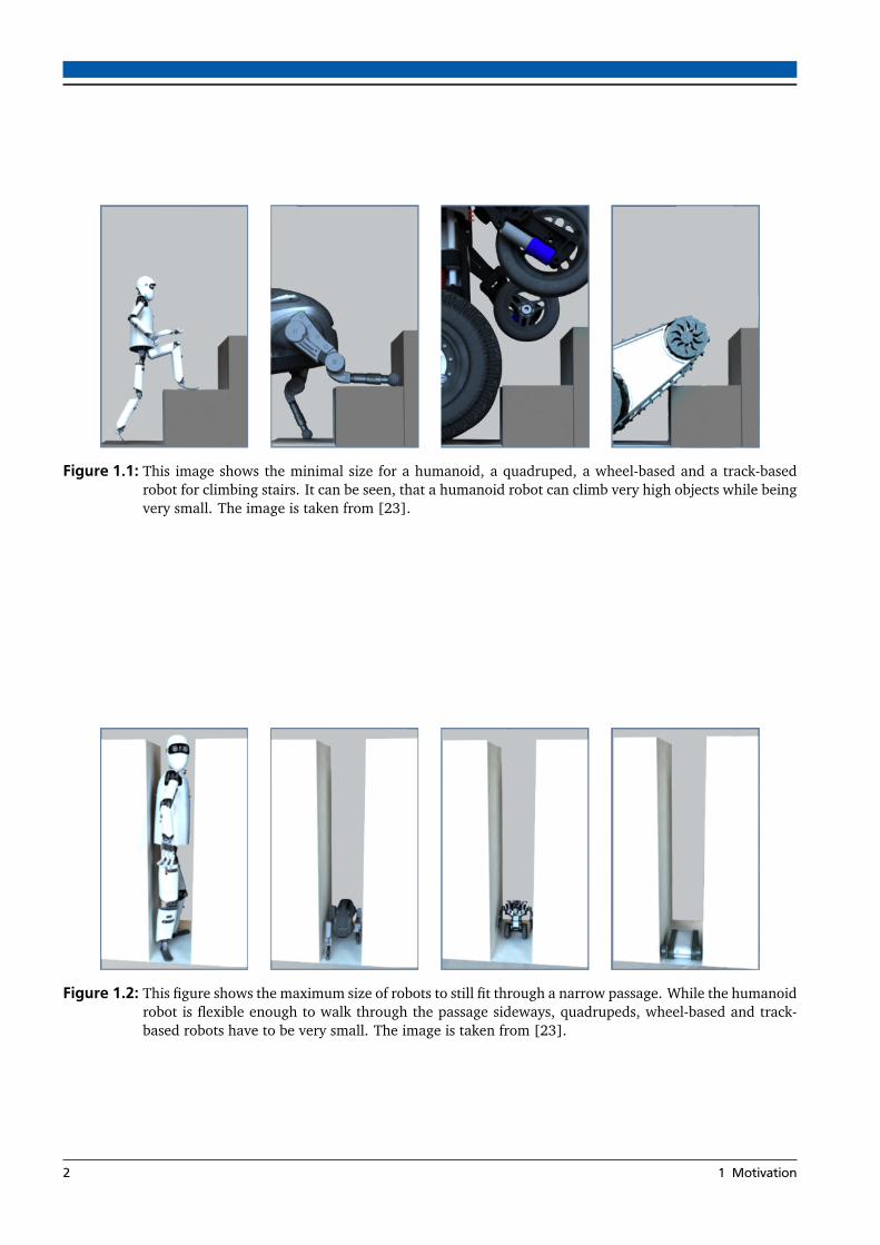
Figure 1.1: This image shows the minimal size for a humanoid, a quadruped, a wheel-based and a track-basedrobot for climbing stairs. It can be seen, that a humanoid robot can climb very high objects while beingvery small. The image is taken from [23].

Figure 1.2: This figure shows the maximum size of robots to still fit through a narrow passage. While the humanoidrobot is flexible enough to walk through the passage sideways, quadrupeds, wheel-based and track-based robots have to be very small. The image is taken from [23].

2 1 Motivation

the feet and on the knees and therefore could kneel down and drive on flat ground. The robot still hada humanoid form and was able to step over objects, climb stairs, use tools and drive the vehicle. TeamKAIST made the first place in the DRC Finals, as they were able to perform the tasks quicker by drivinginstead of walking.Despite of the ability to drive on flat ground, the robot still has to be able to walk in order to benefitfrom the humanoid shape easily. Otherwise, it would not be able to climb stairs or step over gaps andexperience the drawbacks that were already mentioned before.

When operating in a disaster scenario, we might face the problem that the robot has to use a tool tocomplete the mission. For instance, the robot might have to cut a hole through a wall as in the DRC.However, we cannot assume, that we always have access to tools right where they are needed, as it wasthe case in the DRC Finals. The robot might have to pick up a tool from one place and carry it to thetarget place. This means that the robot has to grasp the tool and walk with it to a different location.Obviously, it is important that the robot does not fall during walking.We can also imagine other scenarios where robots have to carry tools or other heavy objects. For instance,a robot for home and industrial use might have to perform pick and place tasks to tidy up a room, sortobjects or pack them for shipping. Also in this case it is important, that the additional weight does notcause the robot to fall over during walking.

3

2 Thesis Overview

We divide this thesis into two goals. The first goal is to get a robot walking by utilizing existing walkingapproaches. The second goal is to extend the approach to enable it to carry objects without falling down.At first, we will present some related work that has been published in both areas in Chapter 3. As wewant to apply all investigated approaches to our THOR-MANG robot, the robot setup is introduced inChapter 4. We will give an overview over both the hardware and the software in that chapter.In Chapter 5 we will cover the most important principles of bipedal walking with robots. We will explaindifferent ways how to model a robot and how to balance it during walking. In Chapter 6 we will explainthree approaches to enable the THOR-MANG to walk without grasped objects. These approaches are theRobotis Walk that comes bundled with the THOR-MANG robot, the Drake toolbox and Missura’s CaptureStep Framework. We will check how applicable those approaches are for our purpose and try to applythem.In Chapter 7 we will explain the steps we took in order to carry an object without falling based on theapproach by Harada et al. [6]. After that, we extend Missura’s Capture Step Framework in order toutilize it to carry objects and take a deeper look on our modifications for the open-loop walk and theclosed-loop controller. In Chapter 8 we present our results and show experiments to evaluate how wellour system of carrying objects performs.In Chapter 9 we conclude this thesis and in Chapter 10 we will give an overview over future steps inorder to improve the system.

5

3 Related Work

Bipedal walking is a deeply investigated research topic. In the last decades, walking controllers havebecome more and more sophisticated. One common characteristic of almost all state of the art walkingcontrollers is the usage of the Zero Moment Point (ZMP) notion [31] to evaluate the balance of the robotand control the gait [12, 18, 5, 8, 6, 38, 35]. A very popular approach is ZMP Preview Control [11],where a ZMP trajectory is used to compute a CoM trajectory that reduces the tracking error. The robotthen tries to follow the CoM trajectory, e.g. by using a Linear Inverted Pendulum Model (LIPM) as robotmodel. For the Model Predictive Control (MPC) approach, Wieber also computes a CoM trajectory from aZMP trajectory, but recomputes the entire trajectory after each iteration based on the current state [33].This approach makes the controller more robust to perturbations. He uses a Quadratic Program (QP)to compute the CoM trajectory, which is computationally expensive but still doable in real time. Mis-sura has presented a pattern generated open-loop walk [1, 21, 18], which is a rather classical approach.While a pure open-loop walk is not state of the art any more, he also developed a closed-loop controllerin parallel, that uses the pattern-based gait and balances the robot using Capture Steps [19, 20, 18, 22].The idea behind Capture Steps is to compensate a disturbance by an adjusted step size when the robotis pushed from any direction. Although this is a very intuitive way of disturbance rejection for humans,the Capture Point was first formalized in 2006 [24] and even later used for walking [7, 4, 20].In contrast to pattern-based walking, there are whole body controllers that can also be used for walking.In general, a whole body controller uses all joints and links of the robot in order to achieve a pre-definedtask. For this purpose, a whole body controller usually has very detailed knowledge about the robotdynamics. As classical control approaches are not applicable for a high DOF system, they often use QPsto generate an optimal solution for a given cost function with respect to a set of constraints (e.g. jointlimits). For Instance, the DRC Teams IHMC and MIT are using whole body controllers for their bipedalAtlas robots [9, 15, 30, 2].

To our knowledge, there are few publications dedicated to walking with grasped objects. Kanehiroet al. described a robot that can carry objects while walking in 1996 [13]. Their walking approach is notstate of the art any more, as they use a pure kinematic pattern generator to generate movements andonly consider the ground projected CoM to stay within the support polygon, not the ZMP. For carryingobjects, they assume the size, weight and CoM of the object to be known.A more recent approach to carry objects has been presented by Harada et al. [6]. They describe a robotthat can perform pick and place tasks. They assume not to know the mass of the object prior to pickingit up and utilize force / torque (F/T) sensors in the hands to estimate the properties of the objects.Additional to special approaches for carrying objects, whole body controllers that use full body dynamicssupport additional weights by design. As long as we can add a model of the grasped object to the robotmodel, the controller can compute a pose that will prevent the robot from falling. In this case, the mostdifficult task is to obtain a precise model of the object, as the robot would have to perform some kind ofcalibration movement [6].

7

4 The Robot Setup

The author of this thesis is a member of Team Hector from Technische Universität Darmstadt in Germany.We participated in the DRC Finals with the THOR-MANG robot named Johnny 05. Thus, we are goingto use that robot for experimentation in this thesis. The robot was developed by Robotis and consists ofstandardized, general-purpose actuators and structural components. We only made minor modificationsto the robot. We removed the additional head LIDAR, upgraded the onboard computer and its PSU andadded a wireless emergency stop and a router as required by the DRC Finals regulations. We also usecustom hands developed by the Virginia Tech. Those hands consist of a stiff wall on the one side and twoactive fingers on the other side. The fingers are underactuated and allow for easy and secure grasping.

The robot is around 1.47 m tall and has a weight of 49.8 kg including all modifications and batteries.The legs have 6 DOF, the arms 7 DOF and the torso 2 DOF.Except for the hands and panning LIDAR, the robot completely uses Robotis Dynamixel Pro servomotorsin different sizes. The robot has a Logitech C920HD Pro Webcam in the head and a Microstrain 3DM-GX3-45 IMU in the pelvis near the CoM. It is also equipped with ATI mini 58 F/T sensors in the anklesand ATI mini 45 F/T sensors in the wrists. Figure 4.1 shows a photo of the robot.

Figure 4.1: The THOR-MANG robot

9

Figure 4.2: We define the global coordinate system as shown in the image. When all joint angles are zero, therobot stands upright with completely stretched knees and the arms hanging to the bottom. In thispose, the joint coordinate systems are aligned with the global coordinate system. The image is takenfrom [18].

We are using the Robot Operating System (ROS) [25] for operating the robot. ROS is a message-oriented middleware that separates each component into a node. Nodes can publish messages to topicsand subscribe to topics to get messages from other nodes. This allows for easy decoupling of softwarecomponents; they might even be distributed over multiple machines and communicate over the network.Communication via ROS topics is not coupled to the internal control loop, which is why ROS providesthe ros_control package. A ROS controller has to implement an update method, which is called at agiven frequency. Thereby, ROS controllers are kept synchronized with the internal control loop. We usea 125 Hz update rate. ROS-Control also defines a hardware_interface for easy access to motors andsensors.

For simulation, we are using GAZEBO 6. GAZEBO can load robots as Universal Robotic DescriptionFormat (URDF) files and is well integrated into ROS. As on the real robot, we can access simulatedhardware from a hardware_interface, execute ROS controllers and control the robot using ROS topics.Therefore, we can use the same code on the real robot and in simulation with only few modifications.For simulating dynamics, we use the default Open Dynamics Engine.

Unless stated differently, we will always assume the following coordinate systems. The robot’s coordi-nate system is right handed with the x-axis pointing to the front of the robot, the y-axis to the left andthe z-axis to the top as shown in Figure 4.2. When all joint angles are zero, the robot stands upright withcompletely stretched knees and the arms hanging downward from the shoulders. In this zero-pose, thecoordinate systems of all joints have the same orientation as the global coordinate system.

10 4 The Robot Setup

5 Foundations of Walking with Bipedal Robots

In this chapter, we will give an overview over important concepts used in a lot of walking algorithms.At first, we will explain two different approaches to model the dynamics of the robot. Most closed-loopwalking controllers use a dynamic model to keep the robot balanced. After that, we will give examplesof two concepts that can be used in order to estimate and preserve the balance of the robot.

5.1 Modelling Robot Dynamics

Not all bipedal walking algorithms use a model of the robot’s dynamics. For instance, Missura andBehnke presented a pattern generator that creates a self-stable open-loop walk using only an abstractkinematic model and hand tuned parameters [21]. Nevertheless, almost all closed-loop controllers re-quire a model of the robot to estimate the impact of a disturbance on the robot and to calculate anappropriate control signal.There are two major classes of dynamic models: Models that only contain limited knowledge and mod-els containing precise knowledge about the dynamic parameters [10]. Firstly, we will give an overviewover the Linear Inverted Pendulum Model (LIPM), which is part of the first family. The LIPM is the mostcommon limited-knowledge-model and is used in many walking and balancing concepts [11, 22, 5, 28].In this thesis, we will utilize the LIPM in Section 6.3 to control the robot. Then we give an overview overthe concept of having a full dynamic model. That concept is relevant for Section 6.2 where we try tocontrol our robot using Drake [30].

5.1.1 Linear Inverted Pendulum Model

The Linear Inverted Pendulum Model is a simplified dynamics model that uses very limited knowledge.It was first formalized by Kajita et al. [10]. The LIPM is derived from the (non-linear) Inverted PendulumModel. The Inverted Pendulum Model assumes the robot to be a point mass rotating around a stick asshown in Figure 5.1a. For the linearization, we assume the mass never moving far from the pivot point.Thus, we assume the point mass having a constant height at all time making the approximation look likein Figure 5.1b. This leads to very simple dynamics:

x = C2 · x (5.1)

with

C =s

gh

. (5.2)

where g = 9.81 m/s2 is the gravitational acceleration and h is the height of the point mass [18]. Kajitaet al. use a more complex definition by including external momentum in their equations [10]. Neverthe-less, most walking concepts that use the LIPM neglect the effects of external momentum.

The linearization also decouples the x and y dimension. Thus, it is possible to construct a two dimen-sional model by combining two one dimensional LIPMs [18]:

�

x

y

�

=

�

C2 0

0 C2

�

·

�

x

y

�

(5.3)

11

(a) Inverted Pendulum (b) Linear Inverted Pendulum

Figure 5.1: The Inverted Pendulum models the robot as a point mass rotating around a stick. The Linear InvertedPendulum neglects the change of the height of that point mass. Both images show the one-dimensionalmodel.

Assuming an undisturbed LIPM, we can calculate both the location and the velocity of the point massat any given time in closed form [18]:

x(t) = x0 cosh (C t) +x0

Csinh (C t) (5.4)

x(t) = x0C sinh (C t) + x0 cosh (C t) (5.5)

x0 and x0 represent the location and the velocity of the point mass at the time t = 0. We can alsocalculate the time when the mass will reach a certain location or have a specific velocity [18]:

t (x) =1C

ln

xc1±

√

√

√x2

c21

−c2

c1

!

(5.6)

t ( x) =1C

ln

xc1C±

√

√

√x2

c21 C2

+c2

c1

!

(5.7)

where

c1 = x0 +x0

C, (5.8)

c2 = x0 −x0

C. (5.9)

Being able to predict the state of the pendulum in closed form is a great advantage when developing aclosed-loop balancing or walking controller, since we can estimate the future movement of the pendulumat any time.

For modelling a robot as Linear Inverted Pendulum (LIP), we need to obtain its CoM. If the movementof the robot is built around a static pose, we can obtain the CoM location as an offset from the robot’s

12 5 Foundations of Walking with Bipedal Robots

pelvis in that static pose and assume it staying constant. This is applicable if the robot does not move toofar from that pose. In order to model movements that are more complex and induce a significant changeof the CoM, we would have to use models that are more complex. For instance, the Extended LIPM [36]uses one LIPM for the torso and each arm of the robot.Especially if the robot is walking, the constant height assumption of the LIPM might not be accurate anymore. Nevertheless, the LIPM has proven to be sufficient for most applications. Johnson et al. even usea LIPM to step over cinder blocks [9], which obviously results in a great change of the CoM height.Wieber has evaluated a whole dynamics model against a simple LIPM while walking with a ZMP-trackingcontroller. The difference between both models stayed within 2 cm on a human sized robot, which waswithin the range of admissible values [33].The LIPM has also been used outside the robotics for human gait analysis and has proven to be sufficientlyaccurate for that application [27].

5.1.2 Full Dynamic Model

In contrast to limited-knowledge-models like the LIPM, a full dynamic model does not make any as-sumptions or approximations on the robot dynamics. Thus, the mass and inertias of every link has tobe known. Determining this model is a hard task, but once obtained it will be more accurate than a LIPM.

Since a full dynamics model contains more information, it can be used for more scenarios than theLIPM. Stephens and Atkeson use a full dynamics model for their Virtual Model Control [28]. By using afull dynamic model, they can directly compute the joint torques from given desired contact forces.Similar to that application, a full dynamics model can be used to reduce the joint tracking error in afeedforward manner. When using a PID controller, the control input is only generated from the errorterm, i.e. if a PID controller is used to track a joint trajectory, there has to be a certain tracking errorto generate a torque in the motors. Even when tracking a constant point, that tracking error might notvanish due to gravitational forces and friction in the joints [9]. In this case, a model can be used tocompute the expected error and compensate it.Since a full dynamics model stays accurate even when the robot changes its pose, we can also use itto obtain a lower dimensional model (e.g. a LIPM). Yi et al. compute the CoM of their robot from adetailed mass model. During manipulation, the robot might extend its arms causing the robot to falleven though the pelvis is not moved. By recalculating the CoM, they are able to move the pelvis in theopposite direction and compensate that effect [38].

A full dynamic model depends on many parameters. When trying to achieve complex goals like walk-ing, this complexity can lead to systems that cannot be solved analytically in real world scenarios, as theanalytic solution does not exist or it is infeasible to solve it. Therefore, some state of the art walking andbalancing controllers use numerical optimization (in the form of quadratic programming) to computedesired joint torques that will fulfill given constraints in the next iteration. While walking, those con-straints are the position and velocity of the CoM or the ZMP that can be computed from the full dynamicmodel. This effectively reduces the full dynamics model to a LIPM again, but enables the controller tocompute a new LIPM in each iteration that better matches the current state of the robot and can includeeffects like arm swinging or other external momentum. An example for a walking controller that uses aQP to track a ZMP trajectory is Drake [30]. We will take a deeper look at Drake in Section 6.2.

5.2 Concepts for Preserving Balance

For this Thesis, there are two concepts of special importance. The first one is the notion of the Zero Mo-ment Point (ZMP) [31]. The ZMP is used in almost all state of the art balancing and walking controllers

5.2 Concepts for Preserving Balance 13

x

y

z

Figure 5.2: A right handed coordinate system where the x-axis points to the front, the y-axis to the left and thez-axis to the top of the foot. Moments and rotations around those axes act in the direction of thecircular arrows.

[12, 18, 5, 8, 6, 38, 35]. The second concept are Capture Steps [24]. Capture Steps can be used inwalking controllers to react to disturbances and regain balance after a push [4, 22, 18].

5.2.1 Zero Moment Point

The ZMP was first mentioned in 1972 by Vukobratovic and Stepanenko in [32], although Vukobratovicalready used the concept in 1968. For the ZMP Notion, we assume the following system: The robot isbalanced, i.e. not falling or tipping around the edge of a foot. The coordinate system is a right-handedsystem with the x-axis pointing to the front, the y-axis to the left and the z-axis to the top of the foot,which is shown in Figure 5.2. When the robot is standing on the ground, the Ground Reaction Force(GRF) consists of the linear force F = (Fx , Fy , Fz) and the moment M = (Mx , My , Mz). Fx , Fy and Mzrepresent the friction force and moment. Because we usually assume those being balanced, we are onlyinterested in the remaining force Fz and moments Mx and My .Using that definition, the ZMP is the point on the ground, where Mx and My are 0, i.e. they are com-pletely expressed by the linear force Fz [31].This point can only exist within the support polygon, because Fz cannot act on a point that is outsidethat polygon. When computing the ZMP from sensor data, there are cases in which the result exceedsthe support polygon. In these cases, the robot will start rotating around the edge of a foot and the resultof the calculation is called Fictional Zero Moment Point (FZMP) [31]. When the ZMP exists, it is alwaysequivalent to the Center of Pressure (CoP) [31].

The notion of the ZMP is used in almost all walking and balancing controllers. When the controllerassures the ZMP staying within the support polygon of the robot at all time, the robot will not fall.For walking algorithms, this leads to a trivial control scheme called ZMP tracking where the walkingtrajectory is represented by a ZMP trajectory. The walking controller can track the ZMP trajectory indifferent ways. For instance by using ZMP Preview Control [11], a CoM trajectory is computed from theZMP trajectory that reduces the ZMP tracking error and the CoM trajectory is tracked instead. Wieberpresented an approach which is called Model Predictive Control or Receding Horizon Control [33]. Healso computes a CoM trajectory from the ZMP trajectory using a QP. After each iteration, the entiretrajectory is recomputed based on the current state, whereby this controller can compensate strongerperturbations than ZMP Preview Control.

14 5 Foundations of Walking with Bipedal Robots

Whenever we compute a CoM trajectory from the ZMP trajectory, we need some kind of robot model.When using a LIPM, the pivot point of the pendulum on the ground is the ZMP. As mentioned earlier,many controllers use a LIPM.

5.2.2 Capture Steps

Pratt et al. introduced the concept of Capture Steps in 2006 as a concept for humanoid push recovery[24]. They defined the Capture Point (CP) as the point on the ground the robot has step to in order tocome to a complete stop. They also defined the Capture Region to be the region of all possible CPs.

Computing the CP is very difficult for complex models. Thus, most publications use a LIPM for thatpurpose [24, 4, 22, 34]. The CP can be calculated from the orbital energy of the LIP [24]:

E =12

x2 −g

2hx2. (5.10)

When the orbital energy is 0, the CoM will come to a rest above the support point of the pendulum. Prattet al. calculate this point to:

xcp = x

√

√hg

. (5.11)

By stepping to the point calculated in Equation 5.11, the robot can reject external disturbances and standstill. We can also use the concept to analyze the current balance of the robot. When the CP is within thesupport polygon, the robot is standing stable [34].

For walking, we usually not want the robot to come to a complete stop but rather return to a nominaltrajectory after it got pushed. Hof presented a controller that uses the CP for walking by calculatinga step duration and CoP position as a function of the CP. The concept was later used by Englsbergeret al. [4]. They expressed the walking trajectory as CP trajectory and developed two ways to control therobot. Their CP End of Step Controller takes only the end of step CP into account and does not dependon future step positions, while the CP Tracking Controller tracks the CP trajectory at all time and tries torealign with the nominal trajectory after a disturbance.Later Missura and Behnke utilized CP tracking for push recovery in their Capture Step Framework [20].They presented a pattern generator for self-stable open-loop walking [21] and added a CP-based con-troller that copes with disturbances by adjusting the step timing and step position. In contrast to Engls-berger et al. [4], they first compute a desired CoM trajectory and compute the CP from that using a LIPM[20].

5.2 Concepts for Preserving Balance 15

6 Walking with THOR-MANG

The first goal of this thesis is to stably walk with a THOR-MANG robot. Robotis already provides awalking approach for the THOR-MANG which is deeper analyzed in Section 6.1. We also tried to adaptboth the Atlas Walking algorithm from Drake [30] and the Capture Step Framework by Missura [18].

6.1 Robotis Walk

The THOR-MANG robot already comes with a walking approach provided by Robotis named RobotisWalk. It implements the ZMP Preview Control scheme that we have explained in the last chapter. TheRobotis Walk is proprietary, i.e. it is only available as binary with headers and we do not have access tothe source code. Additionally, there are no publications regarding this implementation, which makes itextremely hard to adapt to situations it is not designed to work in.The Robotis Walk uses IMU and F/T sensor data as feedback. The F/T sensors are used to always keepthe feet of the robot flush on the ground in order to prevent the robot from lossing traction. Effectively,this results in a certain degree of simulated compliance when the robot gets pushed from either sidewhile it is standing. For instance, if the right F/T sensor measures a higher force than the left sensor, therobot will slightly shorten the right leg.

This simulated compliance is a drawback when walking with grasped objects. If the robot has an objectattached to the right hand, it will apply more weight on the right foot F/T sensor. By shortening the rightleg, the robot will transfer even more weight on that leg and the robot will very likely fall while walking.The desired behavior is to shift the pelvis to the opposite site to move the ground projected CoM in themiddle between the feet again. However, we might also be able to use the compliance to achieve thatbehavior, by simulating different F/T data. We would only have to estimate the properties of the object(mainly the mass and the CoM position with respect to the robot’s pelvis) and add or subtract an offsetfrom the F/T data prior to giving it to the Robotis Walk controller. Thereby, we are able to move the CoMof the robot in the middle again, even if the robot is carrying an object.Unfortunately, the F/T sensors of the robot did not function properly during this thesis and the RobotisWalk is not available in any simulation. Thus, we were not able to investigate whether carrying objectswith simulated F/T data is possible.

6.2 Drake

Our first approach to get THOR-MANG walking with a different algorithm was using the Atlas Walk Al-gorithm from Drake [30]. Drake is a toolbox for analyzing the dynamics of robots and building controlsystems for them. It was developed by the Robot Locomotion Group at MIT, mainly by Tedrake.Drake makes heavy use of optimization based control using quadratic programming. It is written in Mat-lab but uses external .mex code and third party optimizers (SNOPT and Gurobi) for heavy computationtasks.The MIT used the Atlas robot during the DRC Trials and Finals. Thus, although Drake is a general-purpose toolbox, it contains much functionality specific for the Atlas robot. They also used Drake tocontrol the simulated Atlas during the VRC. Among other things, Drake contains a walking controller forAtlas that will be called Drake Atlas Walk for this section.In the next subsections, we will give an overview over the most relevant parts of Drake. We will thenexplain how we applied Drake to THOR-MANG and what problems occurred during the process.

17

6.2.1 Overview

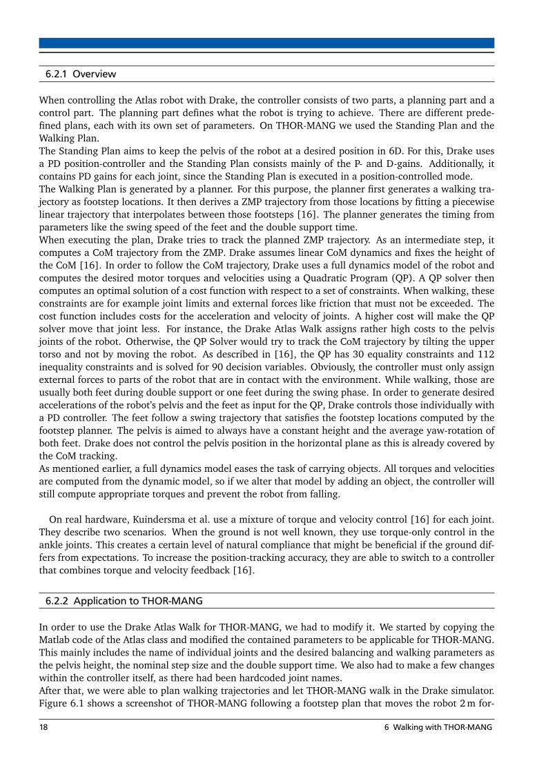
When controlling the Atlas robot with Drake, the controller consists of two parts, a planning part and acontrol part. The planning part defines what the robot is trying to achieve. There are different prede-fined plans, each with its own set of parameters. On THOR-MANG we used the Standing Plan and theWalking Plan.The Standing Plan aims to keep the pelvis of the robot at a desired position in 6D. For this, Drake usesa PD position-controller and the Standing Plan consists mainly of the P- and D-gains. Additionally, itcontains PD gains for each joint, since the Standing Plan is executed in a position-controlled mode.The Walking Plan is generated by a planner. For this purpose, the planner first generates a walking tra-jectory as footstep locations. It then derives a ZMP trajectory from those locations by fitting a piecewiselinear trajectory that interpolates between those footsteps [16]. The planner generates the timing fromparameters like the swing speed of the feet and the double support time.When executing the plan, Drake tries to track the planned ZMP trajectory. As an intermediate step, itcomputes a CoM trajectory from the ZMP. Drake assumes linear CoM dynamics and fixes the height ofthe CoM [16]. In order to follow the CoM trajectory, Drake uses a full dynamics model of the robot andcomputes the desired motor torques and velocities using a Quadratic Program (QP). A QP solver thencomputes an optimal solution of a cost function with respect to a set of constraints. When walking, theseconstraints are for example joint limits and external forces like friction that must not be exceeded. Thecost function includes costs for the acceleration and velocity of joints. A higher cost will make the QPsolver move that joint less. For instance, the Drake Atlas Walk assigns rather high costs to the pelvisjoints of the robot. Otherwise, the QP Solver would try to track the CoM trajectory by tilting the uppertorso and not by moving the robot. As described in [16], the QP has 30 equality constraints and 112inequality constraints and is solved for 90 decision variables. Obviously, the controller must only assignexternal forces to parts of the robot that are in contact with the environment. While walking, those areusually both feet during double support or one feet during the swing phase. In order to generate desiredaccelerations of the robot’s pelvis and the feet as input for the QP, Drake controls those individually witha PD controller. The feet follow a swing trajectory that satisfies the footstep locations computed by thefootstep planner. The pelvis is aimed to always have a constant height and the average yaw-rotation ofboth feet. Drake does not control the pelvis position in the horizontal plane as this is already covered bythe CoM tracking.As mentioned earlier, a full dynamics model eases the task of carrying objects. All torques and velocitiesare computed from the dynamic model, so if we alter that model by adding an object, the controller willstill compute appropriate torques and prevent the robot from falling.

On real hardware, Kuindersma et al. use a mixture of torque and velocity control [16] for each joint.They describe two scenarios. When the ground is not well known, they use torque-only control in theankle joints. This creates a certain level of natural compliance that might be beneficial if the ground dif-fers from expectations. To increase the position-tracking accuracy, they are able to switch to a controllerthat combines torque and velocity feedback [16].

6.2.2 Application to THOR-MANG

In order to use the Drake Atlas Walk for THOR-MANG, we had to modify it. We started by copying theMatlab code of the Atlas class and modified the contained parameters to be applicable for THOR-MANG.This mainly includes the name of individual joints and the desired balancing and walking parameters asthe pelvis height, the nominal step size and the double support time. We also had to make a few changeswithin the controller itself, as there had been hardcoded joint names.After that, we were able to plan walking trajectories and let THOR-MANG walk in the Drake simulator.Figure 6.1 shows a screenshot of THOR-MANG following a footstep plan that moves the robot 2 m for-

18 6 Walking with THOR-MANG

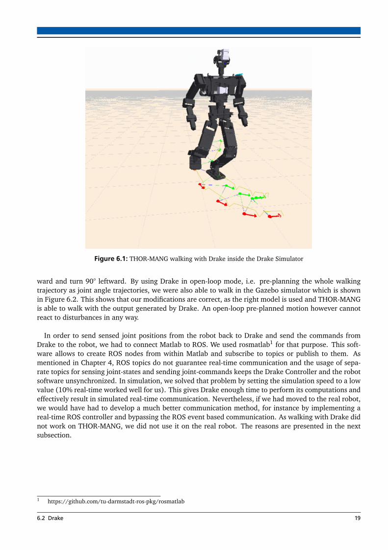
Figure 6.1: THOR-MANG walking with Drake inside the Drake Simulator

ward and turn 90° leftward. By using Drake in open-loop mode, i.e. pre-planning the whole walkingtrajectory as joint angle trajectories, we were also able to walk in the Gazebo simulator which is shownin Figure 6.2. This shows that our modifications are correct, as the right model is used and THOR-MANGis able to walk with the output generated by Drake. An open-loop pre-planned motion however cannotreact to disturbances in any way.

In order to send sensed joint positions from the robot back to Drake and send the commands fromDrake to the robot, we had to connect Matlab to ROS. We used rosmatlab1 for that purpose. This soft-ware allows to create ROS nodes from within Matlab and subscribe to topics or publish to them. Asmentioned in Chapter 4, ROS topics do not guarantee real-time communication and the usage of sepa-rate topics for sensing joint-states and sending joint-commands keeps the Drake Controller and the robotsoftware unsynchronized. In simulation, we solved that problem by setting the simulation speed to a lowvalue (10% real-time worked well for us). This gives Drake enough time to perform its computations andeffectively result in simulated real-time communication. Nevertheless, if we had moved to the real robot,we would have had to develop a much better communication method, for instance by implementing areal-time ROS controller and bypassing the ROS event based communication. As walking with Drake didnot work on THOR-MANG, we did not use it on the real robot. The reasons are presented in the nextsubsection.

1 https://github.com/tu-darmstadt-ros-pkg/rosmatlab

6.2 Drake 19

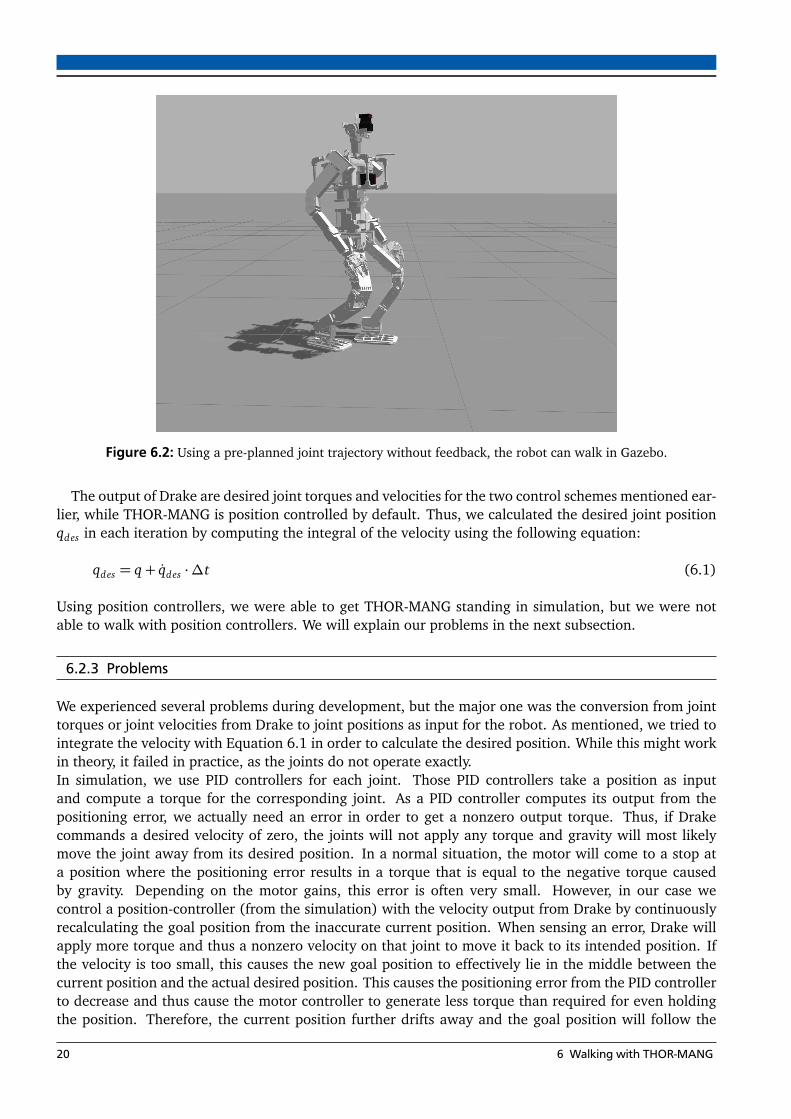
Figure 6.2: Using a pre-planned joint trajectory without feedback, the robot can walk in Gazebo.

The output of Drake are desired joint torques and velocities for the two control schemes mentioned ear-lier, while THOR-MANG is position controlled by default. Thus, we calculated the desired joint positionqdes in each iteration by computing the integral of the velocity using the following equation:

qdes = q+ qdes ·∆t (6.1)

Using position controllers, we were able to get THOR-MANG standing in simulation, but we were notable to walk with position controllers. We will explain our problems in the next subsection.

6.2.3 Problems

We experienced several problems during development, but the major one was the conversion from jointtorques or joint velocities from Drake to joint positions as input for the robot. As mentioned, we tried tointegrate the velocity with Equation 6.1 in order to calculate the desired position. While this might workin theory, it failed in practice, as the joints do not operate exactly.In simulation, we use PID controllers for each joint. Those PID controllers take a position as inputand compute a torque for the corresponding joint. As a PID controller computes its output from thepositioning error, we actually need an error in order to get a nonzero output torque. Thus, if Drakecommands a desired velocity of zero, the joints will not apply any torque and gravity will most likelymove the joint away from its desired position. In a normal situation, the motor will come to a stop ata position where the positioning error results in a torque that is equal to the negative torque causedby gravity. Depending on the motor gains, this error is often very small. However, in our case wecontrol a position-controller (from the simulation) with the velocity output from Drake by continuouslyrecalculating the goal position from the inaccurate current position. When sensing an error, Drake willapply more torque and thus a nonzero velocity on that joint to move it back to its intended position. Ifthe velocity is too small, this causes the new goal position to effectively lie in the middle between thecurrent position and the actual desired position. This causes the positioning error from the PID controllerto decrease and thus cause the motor controller to generate less torque than required for even holdingthe position. Therefore, the current position further drifts away and the goal position will follow the


current position rather than moving the joint back, as in every iteration it lays between the old desiredposition and the current position.For balancing without walking, we can change the joint PD gains Drake uses to compute the desired joint-velocities. By applying high gains, the commanded velocities eventually get high enough to compensatethe effects of gravity. Thus, we were able to get THOR-MANG balancing in simulation. However, ourgoal was to use the walking algorithm of Drake. As explained in Section 6.2.1, the walking controllercomputes the desired velocities by assigning external forces, moving the feet with a PD controller andsolving a cost function with a QP. Thus, we do not have a per-joint PD controller and the robot doesnot operate in a position-controlled mode. For the same reasons as before, the desired position followsthe current position and the robot sinks to the ground when we try to walk. We experimented with aconstant overcompensation variable and computed a new desired position q′des for the motors with theequation

q′des = q+ (qdes ·∆t) · X (6.2)

where X can be chosen freely in order to overshoot the actual desired position and get motor torques thatwould be high enough to at least hold the current position. Again, we were able to execute a standingplan on THOR-MANG without the robot sinking to the ground. Even adaptation to disturbances workedto a certain extent, as the robot would always try to keep the feet on the ground and the pelvis straightupwards even if we tilted the robot. Nevertheless, that concept of constant overcompensation fails forwalking, since the external forces that act on the joints are not constant. Whenever the robot tries totransfer its weight from the middle to the first support foot, the chosen X becomes too small for thesupport leg and too high for the swing leg.Since we have a position-controlled robot, we might not need Drake to keep track of the current motorpositions. Thus, we gave the desired positions of all joints back into Drake and left the actual tracking ofthose positions to the robot itself. At that point, the only real feedback was the pelvis position measuredin world coordinates that Drake uses for the CoM tracking. This improved the motions of the robot, sincethe desired position was not able to follow the current position any more. For the pelvis position howeverwe used the ground truth as computed from the simulator. While this value can be considered exact, itdoes not match the internal model of Drake, which was built with the desired joint states rather thanwith the actual ones. For instance, Drake now thinks that the feet slipped over the ground, as the robotpose has changed, but the pelvis position stayed almost the same due to the actual error in the joints.This causes Drake to not properly shift the pelvis of the robot resulting in a fall as soon as the robotraises the leg. Obviously, we can try to solve that problem by also replacing the real pelvis position withthe desired one, but this would finally degenerate Drake to a pure planning approach with open-loopexecution. We did not try that, as we have already shown that open-loop walking with a pre-plannedtrajectory is possible, but cannot react to external disturbances.

We were not able to solve the transformation from joint velocities to joint positions in a way thatworked for walking. We still think that it is feasible to use the Drake Atlas Walk on THOR-MANG. TheDynamixel Pro Motors actually use a cascaded position controller that is also capable of velocity control,so the next step would be to use the computed velocity as input for the robot. We also would have toextend the simulation to accept a joint velocity as input. We could also try to incorporate the desiredjoint torque without converting it to a position and run the motors in some kind of torque-controlledmode. However, performing torque control on a position-controlled motor is a difficult task. It usuallymeans that we have to determine an accurate model of the motor including the controller and computea position that will make the internal controller generate a given torque. This requires deep knowledgeof the behavior of all mechanical parts like the gearing system, as well as the internal motor controller.Different authors have claimed that torque control with position controlled motors is possible [3, 14],but this would exceed the scope of this thesis. Anyway, considering the Dynamixel Pro motors, it might

6.2 Drake 21

be easier to use those motors in current-control mode as the current is more directly related to the outputtorque than the goal position.Instead of investing additional time into Drake, we decided to use a different walking approach that hasbeen designed for position-controlled robots.

6.3 Missura’s Capture Step Framework

Our second attempt to get THOR-MANG walking was by using Missura’s Capture Step Framework [18].The Capture Step Framework is a closed-loop walking algorithm for omnidirectional walking that targetssoccer robots in the teen-size humanoid RoboCup League. Although those robots are humanoid, theynotably differ from the THOR-MANG. Compared to the THOR-MANG robot, those robots are usuallylightweight and small. Since soccer includes few manipulation tasks and the robots play on flat ground,arms and legs of those robots are usually build very simple and do not have as many degrees of free-dom as the THOR-MANG. For instance, the robot Missura uses for his experiments has legs constructedwith parallel kinematics, which forces the foot to always stay parallel to the hip [18]. In order to in-crease the walking stability, soccer robots often have quite large feet. They usually do not have F/Tsensors in the feet and are only equipped with an IMU. Additionally, soccer robots have low computa-tional power due to restrictions of size. Thus, the Capture Step Framework does not use QP Solversas Drake, but solves all equations in closed form instead. While soccer robots never have to cope withuneven or unknown terrain, they still have to react to sudden disturbances as the robots might hiteach other. As the name implies, the Capture Step Framework uses Capture Steps to reject those distur-bances and keep the robot balanced. The framework also adapts the gait frequency and controls the ZMP.

As the Capture Step Framework uses a LIPM as robot model, we cannot simply add a model of ourgrasped object as it would have been possible in Drake. Nevertheless, the simple design of the CaptureStep Framework along with good code documentation makes it much easier to modify. Thus, we mightbe able to modify the framework and extend it for our purpose. The main advantage over Drake is thatthe Capture Step Framework assumes a position-controlled robot. Therefore, we will not have to handlethe issue of torque to position conversion as in Drake.Unless stated differently, all information regarding the Capture Step Framework in the rest of this sectionare taken from [18].

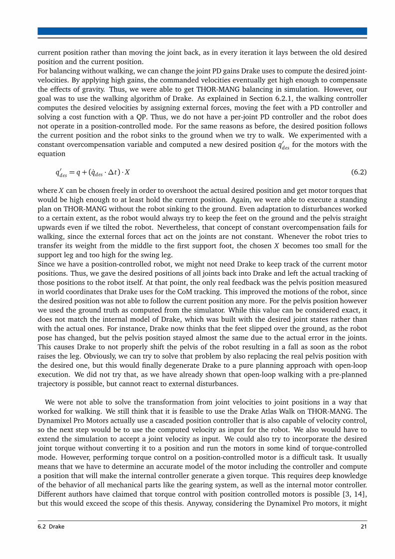
The Capture Step Framework consists of two major components:

1. The Central Pattern Generator (CPG) [1, 21, 18] is a simple open-loop pattern generator thatcreates basic leg movements. It takes a foot placement and a step time as input and creates anomni-directional gait. By tuning many parameters, that gait becomes self-stable, although the CPGcannot actively compensate disturbances.

2. The Footstep Controller [19, 20, 18, 22] actively balances the robot and rejects disturbances. Ituses a LIPM to generate a reference CoM trajectory. When the robot differs from that trajectory, theFootstep Controller balances the robot by calculating appropriate foot placement and step timingvalues as input for the CPG.

Figure 6.3 shows a block diagram of the Capture Step Framework. Both the Central Pattern Generatorand the Footstep Controller are interchangeable. For instance, we can use the CPG in open-loop modewithout any controller or use the Footstep Controller with a different open-loop walking algorithm, aslong as it accepts a foot placement and step timing as input. In the next two chapters, we will take alook at both parts in more detail.


x

y

(q1, . . . , qn)

Robot

c

CPGFootstepController

�

S, T�

Figure 6.3: The Capture Step Framework consists of the CPG and the Foostep Controller. The Footstep Controllersends commands to the CPG in order to balance the robot.

6.3.1 Central Pattern Generator

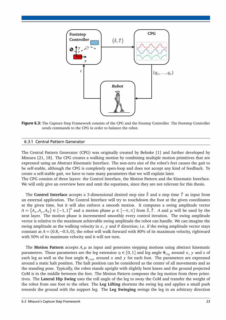
The Central Pattern Generator (CPG) was originally created by Behnke [1] and further developed byMissura [21, 18]. The CPG creates a walking motion by combining multiple motion primitives that areexpressed using an Abstract Kinematic Interface. The non-zero size of the robot’s feet causes the gait tobe self-stable, although the CPG is completely open-loop and does not accept any kind of feedback. Tocreate a self-stable gait, we have to tune many parameters that we will explain later.The CPG consists of three layers: the Control Interface, the Motion Pattern and the Kinematic Interface.We will only give an overview here and omit the equations, since they are not relevant for this thesis.

The Control Interface accepts a 3-dimensional desired step size S and a step time T as input froman external application. The Control Interface will try to touchdown the foot at the given coordinatesat the given time, but it will also enforce a smooth motion. It computes a swing amplitude vectorA =

�

Ax , Ay , Aθ�

∈ [−1,1]3 and a motion phase µ ∈ [−π,π] from S, T . A and µ will be used by thenext layer. The motion phase is incremented smoothly every control iteration. The swing amplitudevector is relative to the maximum achievable swing amplitude the robot can handle. We can imagine theswing amplitude as the walking velocity in x , y and θ direction; i.e. if the swing amplitude vector staysconstant at A= (0.8,−0.5, 0), the robot will walk forward with 80% of its maximum velocity, rightwardwith 50% of its maximum velocity and it will not turn.

The Motion Pattern accepts A,µ as input and generates stepping motions using abstract kinematicparameters. Those parameters are the leg extension η ∈ [0, 1] and leg angle Φleg around x , y and z ofeach leg as well as the foot angle Φ f oot around x and y for each foot. The parameters are expressedaround a static halt position. The halt position can be considered as the center of all movements and asthe standing pose. Typically, the robot stands upright with slightly bent knees and the ground projectedCoM is in the middle between the feet. The Motion Pattern composes the leg motion from three primi-tives. The Lateral Hip Swing uses the roll angle of the leg to sway the CoM and transfer the weight ofthe robot from one foot to the other. The Leg Lifting shortens the swing leg and applies a small pushtowards the ground with the support leg. The Leg Swinging swings the leg in an arbitrary direction

6.3 Missura’s Capture Step Framework 23

using the swing amplitude and motion phase. When walking forward, the support leg moves backwardswith a linear motion and the swing leg swings forward with a sinusoidal motion to create a smooth gait.To prevent the foot from scratching over the ground, the swing phase is delayed to start shortly after thefoot is lifted off the ground and ends before the touchdown.

The Abstract Kinematic Interface accepts the leg extension η, leg angle Φleg and foot angle Φ f oot foreach leg as input and converts those abstract kinematic parameters to joint angles. The leg extension isfrom the interval [0, 1]. A leg extension of 0 represents a stretched leg, while 1 means that the leg isfully retracted. The reference coordinate system for the leg angle and the foot angle is the robot’s pelvis.This creates an easy way to express swing trajectories, because changing the leg angle for swinging theleg forward preserves the orientation of the foot with respect to the pelvis without any additional cal-culations. The Abstract Kinematic Interface is mainly model free. It only assumes the thigh and shankof the robot having equal length and all joints being beneath each other on a vertical line when all jointangles are zero. Thus, the actual outcome of the CPG as the step size or the step height depends on therobot.

6.3.2 Footstep Controller

The Footstep Controller receives the current state from the robot, evaluates the current balance and cal-culates appropriate inputs for the CPG. The Footstep Controller uses a LIPM, which is why the currentstate of the robot is represented by the CoM state c and consist of the ground projected centroid positionand the velocity. It is important to know, that the Footstep Controller does not aim to track the real CoMof the robot but assumes the ground projected middle point between the hip joints to be the groundprojected CoM, instead. It also assumes the IMU sitting between the hip joints. Missura claims that thisis sufficient, as all disturbances that act on the CoM will also act on that point between the hip joints[18]. Thereby, we can track any arbitrary point on the robot to evaluate its balance.

The Footstep Controller maintains three robot-states, each consisting of the ground projected centroidposition and velocity as mentioned above:

1. The rx-state is the state the Controller receives from the robot. The Controller does not directlyoperate on that state.

2. The mx-state is the model state that aims to reduce noise. The model state is a mixture of thereal rx-state and a pure LIPM driven robot model. In each iteration, the controller computes a newmx-state by assuming that the robot will behave like a perfect LIPM for the time of one controliteration. Then, the Footstep Controller interpolates linearly between the mx-state and the rx-statewith a blending factor b. Thus, the Controller can base its calculations on the noise-free open-loopmodel when the rx-state evolves as expected. It is also used closely before and after the supportexchange, as this causes additional noise.

3. The tx-state is the actual state the controller is working on. It is the expected state the robot shouldhave when the motors executed the commands. It is calculated by using the mx-state as start andassuming, that the robot will behave like a perfect LIPM for the time span of a predefined latencyl. The latency is the complete latency of the system including communication latency and the timethe motors need to execute commands. We have to manually determine l when tuning the FootstepController. Compliant actuation has a significant effect on the latency, as the motors might needmore time to execute commands.

The connection between those three robot states is illustrated in Figure 6.4.


rx mx tx 𝑙

1

𝑏𝑙𝑒𝑛𝑑

b

Figure 6.4: This diagram shows the calculation of the tx-state the controller operates on. The circular blocksrepresent a prediction of the future (one iteration or l seconds ahead) under the assumption that therobot behaves like a perfect LIPM.

In order to evaluate the balance of the robot and compensate disturbances, the Footstep Controllertracks the CoM and steers it towards a reference trajectory. The Footstep Controller assumes the robotacting as a perfect LIPM unless disturbed. As explained in Section 5.1.1, using a LIPM decouples sagittaland lateral motions. Those motions differ notably from each other as shown in Figure 6.5. In the lateraldirection, the CoM oscillates between the two pivot points of the pendulum, but never crosses them. Ifthe CoM would cross the pivot point, the robot would fall. In the sagittal direction, the CoM crosses thepivot point in each step. In order to describe the CoM trajectory, the Capture Step Framework uses fourparameters of which three are used to describe the lateral motion and one is used for the sagittal motion.

The lateral motion is shown in Figure 6.5a. The minimum lateral distance of the CoM to the pivotpoint of the LIP is called α. This is the lateral pendulum apex and the lateral CoM velocity is zero at thatpoint. The lateral support exchange happens at a location from the interval [δ,ω]. We can consider thisthe half step width. At the point of support exchange, the lateral CoM velocity reaches its maximum.When not walking sideward, the support exchange always happens at the distance δ. When walkingsideward, the robot takes a larger leading step with a support exchange at a distance up to ω. Thetrailing step will again aim to cause a support exchange at δ.We only need one parameter to model the sagittal motion as shown in Figure 6.5b. σ denotes the max-imum sagittal CoM distance from the pivot point and thus can be considered the maximum half steplength. The sagittal support exchange will happen at a distance within [0,σ] depending on the sagittalwalking velocity. At that point, the sagittal CoM velocity is at maximum.The Capture Step Framework aims not to force an unnatural oscillation on the robot. Thus, we have totune the parameters α,δ,ω,σ manually to represent the undisturbed movements of the robot as pre-cisely as possible. In Section 6.3.3 we will explain how to obtain those parameters.

Since the ZMP is the pivot point of the pendulum, the Controller can use that point to influence themovement of the CoM. It just has to enforce that the ZMP always lies within the support polygon ofthe feet. Since the Capture Step Framework does not model a double support phase, the ZMP has tobe within the area of the current support foot. The Capture Step Framework always assumes the ZMPstaying constant during a whole step.The lateral ZMP is computed, so that the CoM reaches the lateral support exchange location at the nomi-nal step time. For this, the Footstep Controller uses the LIPM location predictor equation (Equation 5.4).When the disturbance is strong enough, there are several cases when the nominal time, the nominalsupport exchange location or both cannot be met. These cases happen because the foot size is limitedand the ZMP cannot be positioned outside the convex hull of the support foot. If the controller detectssuch a case, it chooses another support exchange location and computes a new predicted step time. Thisnew predicted step time is used for all further calculations, so the lateral movement controls the timingof the gait.


δ (sidewards walking: ω)α

Lateral:

(a) The Lateral motion can be described by three paremeters. α is the minimal distance to the pen-dulum pivot point, the CoM may have. When walking in place, the support exchange happenswhen the CoM is at distance δ to the pivot point. When walking sideward, the support exchangehappens at a distance from the interval [δ,ω].

σ

Sagittal:

(b) For the sagittal motion, we only need one parameter to describe the pendulum. σ is the maximumhalf step size, i.e. when walking forward, the support exchange happens at a distance from [0,σ].

Figure 6.5: The lateral and sagittal motion of the robot behave notably different. For the lateral motion, the CoMnever crosses the pivot point of the pendulum, while for the sagittal motion, the CoM crosses that pointin every step.

The sagittal ZMP is computed so that the CoM will arrive at the sagittal support exchange location atthe predicted step time that is taken from the lateral direction.It is notably, although Missura’s Capture Step Framework calculates the ZMP location in every controliteration, this mainly remains a theoretical construct. The Footstep Controller does not enforce the ZMPto actually be at that position. Measuring the real ZMP was not possible for Missura, since soccer robotsusually do not have F/T sensors in the feet. Thus, the computed ZMP is only used to check, if the footplacement has to be modified, i.e. if the robot has to perform a Capture Step.

In order to calculate the footstep location, the controller uses the predicted step time and ZMP loca-tion calculated in the previous step and the current CoM-state c. From those values, it calculates theachievable end-of-step CoM-state c′ =

�

c′x , c′x , c′y , c′y�

. That achievable CoM-state might differ from thenominal state, as the robot might not be able to compensate a disturbance completely by relocating theZMP.For the sagittal footstep location, the controller first computes the sagittal velocity at the pendulumapex that would result in the achievable end-of-step velocity using the LIPM velocity predictor equation(Equation 5.5). Since sagittal steps are symmetrical, that velocity can be used with the LIPM locationpredictor equation (Equation 5.4) to compute the end-of-step location. The controller calculates thelateral footstep location so the CoM will pass the apex of the next step at the distance α. For this, itassumes the orbital energy (Equation 5.10) to stay constant at all times, i.e. the orbital energy right afterthe support exchange is equal to the orbital energy at the lateral apex.The Footstep Controller does not control the rotation of the robot. It assumes the rotation being smallenough to have no effect on the robot’s balance and simply passes it through.


6.3.3 Application to THOR-MANG

We successfully applied Missura’s Capture Step Framework to THOR-MANG. Although we had to makesome modifications on the Capture Step Framework, most of the work was tuning the Central PatternGenerator and the Footstep Controller. This requires deep knowledge about the Capture Step Frameworkand an understanding of what the robot is supposed to do and how the graphs have to look like in order toachieve a stable gait. Some parameters have to be tuned in a certain order. In the following subsections,we will explain how we got THOR-MANG walking, but the technique can also be applied to other robots.

Preparations

Missura provided us with his implementation of the Capture Step Framework, so we did not have toreimplement it based of his papers. Nonetheless, we had to implement a communication interface be-tween the robot and the Capture Step Framework. As it is quite simple to get the data out of the CaptureStep Framework using a UDP socket, our first attempt was to implement a ROS node that acted as abridge by converting data from the Capture Step Framework and sending it to the robot via ROS topics.This was not suitable due to the limited real-time capabilities of the event based communication in ROS,and we developed a UDP Controller as ROS-Controller instead. The UDP Controller runs on the robot’sonboard computer and communicates with the Capture Step Framework application via UDP. The com-munication is fast enough to stay synchronized with the robot’s main control loop at 125 Hz without anyproblems, even though the Capture Step Framework runs on a different computer and is connected withan Ethernet cable.

As mentioned in Section 6.3.1, the Abstract Kinematic Interface of the CPG assumes equal lengthof thigh and shank of the robot, as well as all joints being on a straight vertical line when the anglesare zero. While THOR-MANG meets the first requirement, the knee motor violates the latter which isillustrated in Figure 6.6a. Thus, we added an option to the Capture Step Framework to compensate themisalignment by redefining the zero pose. The offset for the hip pitch and ankle pitch is

∆q = −arcsin�

0.03p

0.32 + 0.032

�

= −0.0997 rad (6.3)

and the offset for the knee is −2 ·∆q. Figure 6.6b illustrates the new zero pose with compensated jointmisalignment. Obviously, the redefined zero pose also causes a change of the leg length which howeveris not a problem, as the CPG does not use any robot model.

We discovered that the motor gains are of special importance for the gait quality, both in simulationand with the real robot. We can set custom control-parameters in the Dynamixel Pro motors, but at thetime we started working with the robot, the onboard software did not provide an easy option for that.Therefore, we implemented a ROS Dynamic Reconfigure server that enables us to configure control-gains.The Dynamixel Pro motors accept three gains that are called position P gain, velocity P gain andvelocity I gain. Since Robotis does not provide further information regarding the controller, wereverse-engineered it experimentally. The controller is a cascaded velocity and position controller asshown in Figure 6.7. When setting a desired position, the controller first computes a desired velocityusing a P-controller. The velocity is controlled using a PI control loop.


0.3 m

0.3 m

0.03 m

(a) Original zero-pose

Front

(b) New zero-pose

Figure 6.6: The knee joint of the THOR-MANG robot has an offset towards the back. Since the CPG assumes alljoints being at a vertical line when the angles are zero, we have to redefine the zero pose.

𝑃𝑝𝑜𝑠 𝑃𝑣𝑒𝑙

𝐼𝑣𝑒𝑙 ⋅ 𝑥 dt

Motor 𝑞

−

𝑞 𝑞

− 𝑞

𝐼

Figure 6.7: The controller of the Robotis Dynamixel Pro motors is a cascaded position and velocity controller. Theposition control loop is a simple P-controller that computes a desired velocity. The velocity controlleris a PI controller.

Tuning the Central Pattern Generator

The Central Pattern Generator is responsible for the open-loop gait of the robot. As mentioned earlier,the open-loop walk has to be self-stable, as we determine the LIPM of the robot from this gait. The CPGbuilds its motions around a static halt position, so we need to tune both the halt position and the motiongeneration. In this section, we will go over the important parameters and explain how we tuned them.

At first, we have to tune an arbitrary halt position. There are only three constraints for that position:

1. The ground projected CoM of the robot has to be in the middle between the feet. Obviously, therobot must not fall while standing.

2. The legs have to be spread apart slightly.3. The knees must at least be bent slightly.

The halt position is expressed in abstract kinematic parameters as explained in Section 6.3.1. Originally,the CPG offers the leg angle and foot angle that are both two-dimensional around the x and y axis andthe one-dimensional leg extension to express the halt positon. The weight of THOR-MANG’s upper bodyis not centered above the hip joints, as the batteries and the computer are on the back. Thus, we found


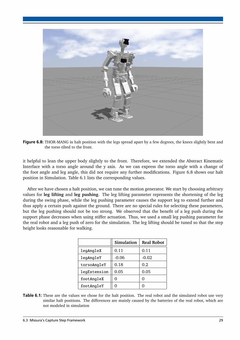
Figure 6.8: THOR-MANG in halt position with the legs spread apart by a few degrees, the knees slightly bent andthe torso tilted to the front.

it helpful to lean the upper body slightly to the front. Therefore, we extended the Abstract KinematicInterface with a torso angle around the y axis. As we can express the torso angle with a change ofthe foot angle and leg angle, this did not require any further modifications. Figure 6.8 shows our haltposition in Simulation. Table 6.1 lists the corresponding values.

After we have chosen a halt position, we can tune the motion generator. We start by choosing arbitraryvalues for leg lifting and leg pushing. The leg lifting parameter represents the shortening of the legduring the swing phase, while the leg pushing parameter causes the support leg to extend further andthus apply a certain push against the ground. There are no special rules for selecting these parameters,but the leg pushing should not be too strong. We observed that the benefit of a leg push during thesupport phase decreases when using stiffer actuation. Thus, we used a small leg pushing parameter forthe real robot and a leg push of zero for the simulation. The leg lifting should be tuned so that the stepheight looks reasonable for walking.

Simulation Real Robot

legAngleX 0.11 0.11

legAngleY -0.06 -0.02

torsoAngleY 0.18 0.2

legExtension 0.05 0.05

footAngleX 0 0

footAngleY 0 0

Table 6.1: These are the values we chose for the halt position. The real robot and the simulated robot use verysimilar halt positions. The differences are mainly caused by the batteries of the real robot, which arenot modeled in simulation


The next step is to select arbitrary values for the lateral and sagittal swing slope. Those parameterscause the robot to swing the leg in lateral or sagittal direction depending on the commanded gait velocity.The value is mainly important for walking in open-loop mode where a gait velocity of one representsmaximum speed. Again, we tune those parameters, so that the outcome looks reasonable. When walkingat full speed, our THOR-MANG robot moves at approximately 0.2 m per step.At last, we have to tune the step frequency and lateral hip swing. Those parameters are extremelyimportant for a stable open-loop gait and have to be tuned in parallel as they influence each other. Thegoal of this step is to get a stable oscillation of the robot in lateral direction. This oscillation will laterprovide the reference timing and CoM movement for the Footstep Controller. To our knowledge, allrobots the Capture Step Framework has been applied to, use a step frequency from 2.0 Hz to 2.5 Hz, soit seems like good practice to start with a value from within that range. Without any lateral hip swing,the robot will now perform a walking motion, but it will not shift its weight from one foot to the otherproperly. Thus, we can raise the lateral hip swing, until we get a lateral oscillation that looks smooth.The feet should always hit the ground in plane. If the feet lift at one edge, the lateral hip swing is too lowor too high. After this first rough tuning step, we can fine-tune the oscillation. The goal is to get a goodrepetitive movement of the CoM. The support exchange should always happen at the same time and theCoM should always be at the same location at that time. Figure 6.9 shows the CoM y component of theCoM state and the roll angle of the robot as reported by the IMU for a non-perfect oscillation. The CoMstate is relative to the current support foot causing the graph to jump and displaying the time of supportexchange. The robot is walking in place at 2 Hz. We can clearly see the spikes of the CoM y value and thelocal minima and maxima of each step being at different heights. This is undesired, since the FootstepController will later estimate the balance of the robot based on those values. If they show irregularbehavior, the Footstep Controller will assume that the robot has been disturbed and try to compensatethe disturbance by adapting the step timing and foot placement. The IMU roll angle is not important forthe Footstep Controller, but we figured out that it is a good indicator to see if we found a good oscillation.Figure 6.9 clearly shows an IMU roll angle with an irregular behavior. Figure 6.10 shows the same robotafter fine-tuning the CPG. The IMU roll angle shows a regular oscillation synchronized with the steppingmotion and the CoM y curve looks the same in every step. In this state, we can apply small disturbancesand the robot will return to that oscillation after some time. Getting this behavior requires exhaustivetuning by modifying the lateral hip swing and step frequency. We achieved the result from Figure 6.10mainly by trial and error, i.e. trying a different step frequency and retuning the lateral hip swing. Wefigured out that a higher step frequency often requires a lower lateral hip swing and vice versa.

After we have created a stable lateral oscillation, the robot should be able to walk self-stable. If ittends to tilt when walking forward or backward, we can adjust the halt position slightly to move theCoM to the back or to the front. Table 6.2 shows our values for the simulated and the real robot. Themain difference between both are the lateral hip swing and the gait frequency, which are also the mostimportant parameters. The difference is primarily caused by different motor parameters for hip roll andankle roll motors, as the simulated robot uses stiffer actuation.

Tuning the Footstep Controller

As explained earlier, the Footstep Controller uses a CoM reference trajectory to analyze the balance ofthe robot. It then computes a ZMP and adapts the step timing and foot placement to steer the robottowards that reference trajectory. Since the Footstep Controller only receives the current CoM state fromthe robot, we need to set all values representing the undisturbed robot manually. Those values are thependulum constant C2 from Equation 5.1, the latency l from Section 6.3.2 and the values α,δ,ω and σthat represent the CoM trajectory as shown in Figure 6.5.


−0.2

0

0.2 CoM y

0 1 2 3 4 5 6 7 8 9 10−4−2

0

2

4

time [s]

IMU roll [°]

Figure 6.9: A non-harmonic lateral oscillation prevents the robot from walking self-stable. The CoM y value hasspikes at different heights and the IMU roll angle shows an irregular behaviour. The CoM position isalways measured with respect to the current support foot and thus jumps whenever the robot takes astep.

−0.2

0

0.2 CoM y

0 1 2 3 4 5 6 7 8 9−4−2

0

2

4

time [s]

IMU roll [°]

Figure 6.10: When we successfully tuned the lateral oscillation, the CoM y value will roughly look the same atevery step and all spikes are at the same height. A regular IMU roll angle is a good indicator to seeif we found the perfect oscillation. Again, we measure the CoM position with respect to the currentsupport foot.



gaitFrequency 2 2.3

pushHeight 0 -0.01

stepHeight 0.1 0.1

stepLengthYSlope 0.08 0.08

stepLengthZSlope 0.2 0.2

stepLengthXSlopeFwd 0.2 0.2

stepLengthXSlopeBwd 0.2 0.2

lateralHipSwing 0.096 0.132

Table 6.2: These are the values we chose for the CPG. The difference of the lateral hip swing and gait frequency ismainly caused by different motor stiffness.

0 0.5 1 1.5 2 2.5 3 3.5 4 4.5 5 5.5 6

−0.2

0

0.2

α δ

time [s]

CoM y

Figure 6.11: By looking at recorded data of the robot walking in place open-loop, we can directly obtain the correctvalues for α and δ. δ is the maximum CoM displacement and α is the minimum CoM displacementfor each step.

At first, we need to tune the lateral trajectory. As we have already tuned a self-stable CPG, we want theFootstep Controller to replicate that motion as closely as possible; respectively we want the controllernot to adapt the foot placement unless the robot is disturbed.We begin with tuning the pendulum apex α and the half step width δ. For this purpose, we let therobot walk in place in open-loop mode and record the lateral CoM movement. As explained earlier, δis the half step width, respectively the maximum CoM displacement from the current support foot whennot walking sideward. Thus, we can determine δ to be the maximum values of the recorded CoM y data.Analogously, α is the CoM apex in lateral direction, respectively the minimum CoM displacement whennot walking sideward. Figure 6.11 shows the recorded lateral CoM data from the previous figure. Thedashed lines show the values for α and δ. The controller uses only one value α and δ for both supportfeet. Therefore, the walking trajectory must be symmetrical while walking in place. The figure showswell how the local extrema and spikes of each step line up with the dashed lines both on the top and onthe bottom.

In the next step, we need to tune the maximum half step width ω. Again we can obtain thatparameter from walking in open-loop mode, but as ω only affects sideward walking, we have to walksideward with maximum speed (the lateral walking velocity has to be 1). Figure 6.12 shows the CoM ymovement for a robot while walking leftward at maximum speed. Since the leading step is longer, thelarger spikes represent the maximum CoM displacement.


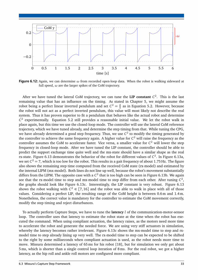
0 0.5 1 1.5 2 2.5 3 3.5 4 4.5 5 5.5 6

−0.2

0

0.2ω

time [s]

CoM y

Figure 6.12: Again, we can determine ω from recorded open-loop data. When the robot is walking sideward atfull speed, ω are the larger spikes of the CoM trajectory.

After we have tuned the lateral CoM trajectory, we can tune the LIP constant C2. This is the lastremaining value that has an influence on the timing. As stated in Chapter 5, we might assume therobot being a perfect linear inverted pendulum and set C2 = g

h as in Equation 5.2. However, becausethe robot will not act as a perfect inverted pendulum, this value will most likely not describe the realsystem. Thus it has proven superior to fit a pendulum that behaves like the actual robot and determineC2 experimentally. Equation 5.2 still provides a reasonable initial value. We let the robot walk inplace again, but this time we use the closed-loop mode. The controller will use the lateral CoM referencetrajectory, which we have tuned already, and determine the step timing from that. While tuning the CPG,we have already determined a good step frequency. Thus, we use C2 to modify the timing generated bythe controller to achieve the same frequency again. A higher value for C2 will raise the frequency as thecontroller assumes the CoM to accelerate faster. Vice versa, a smaller value for C2 will lower the stepfrequency in closed-loop mode. After we have tuned the LIP constant, the controller should be able topredict the support exchange time quite well and the mx-state should have a similar shape as the realrx-state. Figure 6.13 demonstrates the behavior of the robot for different values of C2. In Figure 6.13a,we set C2 = 7, which is too low for the robot. This results in a gait frequency of about 1.75 Hz. The figurealso shows the remaining step time computed from the received CoM state (rx-model) and estimated bythe internal LIPM (mx-model). Both lines do not line up well, because the robot’s movement substantiallydiffers from the LIPM. The opposite case with a C2 that is too high can be seen in Figure 6.13b. We againsee that the rx-model time to step and mx-model time to step differ from each other. After tuning C2,the graphs should look like Figure 6.13c. Interestingly, the LIP constant is very robust. Figure 6.13shows the robot walking with C2 ∈ [7,16] and the robot was able to walk in place with all of thosevalues. Considering a perfect LIP, the resulting range of the CoM height is between 0.6 m and 1.4 m.Nonetheless, the correct value is mandatory for the controller to estimate the CoM movement correctly,modify the step timing and reject disturbances.

To actually perform Capture Steps, we have to tune the latency l of the communication-motor-sensorloop. The controller uses that latency to estimate the robot state at the time when the robot has exe-cuted the command. When using compliant actuation, the latency raises, as the motors need more timeto accelerate the robot and generate the needed force. We are using very stiff actuators in simulation,whereby the latency becomes rather irrelevant. Figure 6.13c shows the mx-model time to step and rx-model time to step already lining up very well. The rx-model time to step can be expected to be shiftedto the right by some milliseconds when compliant actuation is used, as the robot needs more time tomove. Missura determined a latency of 65 ms for his robot [18], but for simulation we only get about5 ms, which is shorter than a single control loop iteration of 8 ms. For the real robot, we got a higherlatency, as the hip roll and ankle roll motors are configured more compliant.


1.5

2

2.5

3 Gait Frequency [Hz]

0 0.5 1 1.5 2 2.5 3 3.5 4 4.5 5 5.5 60

1

2

3

time [s]

rx-model time to step [s]mx-model time to step [s]

(a) If C2 is too low, the robot steps too slowly. We can also see the poor estimation of the remaining time to step, i.e. therobot does not behave like the internal LIPM. In this figure C2 is 7.

1.5

2

2.5


0 0.5 1 1.5 2 2.5 3 3.5 4 4.5 5 5.5 6−0.2

0

0.2

0.4

time [s]


(b) If C2 is too high, the robot steps too fast. Again, we can observe that the movement of the robot differs from the LIPMby looking at the remaining step time. In this figure C2 is 16.

1.5

2

2.5


0 0.5 1 1.5 2 2.5 3 3.5 4 4.5 5 5.5 60

0.20.40.6

time [s]


(c) A correctly tuned C2 value of 8.2 gives us approximatley the same gait frequency as the open-loop walk.

Figure 6.13: For tuning the LIP constant C2, we let the robot walk in closed-loop mode and try to reproduce thestep frequency that we have chosen originally when tuning the CPG. A higher C2 makes the robotstep faster and vice versa. This figure is from our simulated robot, so the CPG gait frequency is 2 Hz.


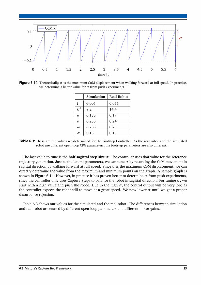
0 0.5 1 1.5 2 2.5 3 3.5 4 4.5 5 5.5 6

−0.1

0

0.1

σ

time [s]

CoM x

Figure 6.14: Theoretically, σ is the maximum CoM displacement when walking forward at full speed. In practice,we determine a better value for σ from push experiments.


l 0.005 0.055

C2 8.2 14.4

α 0.185 0.17

δ 0.235 0.24

ω 0.285 0.28

σ 0.13 0.15

Table 6.3: These are the values we determined for the Footstep Controller. As the real robot and the simulatedrobot use different open-loop CPG parameters, the footstep parameters are also different.

The last value to tune is the half sagittal step size σ. The controller uses that value for the referencetrajectory generation. Just as the lateral parameters, we can tune σ by recording the CoM movement insagittal direction by walking forward at full speed. Since σ is the maximum CoM displacement, we candirectly determine the value from the maximum and minimum points on the graph. A sample graph isshown in Figure 6.14. However, in practice it has proven better to determine σ from push experiments,since the controller only uses Capture Steps to balance the robot in sagittal direction. For tuning σ, westart with a high value and push the robot. Due to the high σ, the control output will be very low, asthe controller expects the robot still to move at a great speed. We now lower σ until we get a properdisturbance rejection.

Table 6.3 shows our values for the simulated and the real robot. The differences between simulationand real robot are caused by different open-loop parameters and different motor gains.


7 Carrying Objects

At this point, THOR-MANG is able to walk stably and recover from pushes using Capture Steps. Asexplained in Chapter 2, carrying objects with the robot is the second goal of this thesis. Consideringthe disaster scenario from the DRC, the robot might have to use tools that are not located next to theoperation site.Carrying objects was not that important for the DRC itself. The robots just had to cut a hole in a wallusing a battery powered DEWALT cutout tool or a drill. Those tools were located right next to the wall,so the robots did not have to move much after grasping the tool. Additionally, many teams used theAtlas robot from Boston Dynamics, which weights around 180 kg. The tools only weight about 1.5 kgin comparison. In this thesis, we will use a much lighter robot and assume heavier tools. We also as-sume no model of the object to be known, i.e. we know neither the weight, nor the location of the CoMor the inertia of the object. This applies to a real life situation where the robot has to use an arbitrary tool.

When a robot is carrying a grasped object, this object acts a constant force and moment on the robot.Since we cannot assume the object being in the CoM of the robot, the additional weight causes a CoMdisplacement in the corresponding direction. If the ground projected CoM position exceeds the supportpolygon in a static stance, the robot will fall down. When the robot is walking, the effect of an additionalmass will be even more relevant because a gait is naturally less stable and usually requires active controlto balance the robot due to the smaller support polygon and external disturbances. Thus, an object mightcause the robot to fall when walking, even if the robot is still able to stand.

7.1 Approach by Harada et al.

As already mentioned in Chapter 3, not many publications dedicated to walking with grasped objects areavailable. The approach by Kanehiro et al. is not state of the art anymore and assumes the size, weightand CoM of the object being known [13].In contrast, the approach by Harada et al. does not make those assumptions [6]. In order to measure theproperties of the object, they use F/T sensors in the hands. Although their hardware is able to measurethe moment created by the object, they neglect that effect and only include linear forces of the hand F/Tsensors in their equations. Thereby, they always assume the CoM of the object being vertically beneath orabove the hands. Obviously, this produces an inaccurate result whenever the robot grasped the object ata different position. For walking, Harada et al. plan a ZMP trajectory without considering the additionalmass. Using the estimated weight of the object, they create a new model of the robot including theobject. By moving the robot’s pelvis, they compensate the CoM displacement prior to walking and usetheir ZMP-tracking controller without further modification. Summarized, Harada et al. use three stepsto cope with grasped objects:

1. Estimate the mass model of the object while the robot is not moving2. Fuse the robot model with the object to obtain a combined model (represented by a ZMP offset)3. Move the waist to bring the ZMP in the middle between the feet again

Actually, we are not interested in a dedicated mass model of the grasped object, as we would just fuseit with the robot model anyway. It might be possible to directly obtain the combined model using F/Tsensors in the feet, thus for this thesis we will reduce the three steps from Harada et al. to the followingtwo:

1. Obtain the combined model including the object2. Compensate the effects of the object e.g. by moving the waist

We will take a deeper look on how to achieve those two steps in the next two subsections.

37

7.1.1 Obtaining the new Robot Model

As already explained in Section 5.1, there are different types of models. If we are using a full dynamicsmodel, we just have to add the dynamics of the grasped objects to that model in order to obtain thecombined model. However, determining a precise model of the object is very difficult. Using 6-axis F/Tsensors in the hands, we can only measure the weight of the object and the CoM location in the horizon-tal plane, i.e. we cannot calculate the height of the CoM from that data [6]. In order to determine thecentroid height, the robot has to turn the object, obtain another horizontal CoM location and computethe 3D CoM location using a triangle equation. A full dynamic model would also require the inertias ofthe object. In order to determine those, the robot has to perform calibration movements and measurethe resulting F/T data.As we did not succeed in walking with Drake, our controller does not use whole body dynamics. ForMissura’s Capture Step Framework, we need to obtain the LIPM of the robot, which can be achieved ineasier ways.

If the controller relies on a low dimensional model like a LIPM or continuously reduces a complexmodel to a single CoM, it might be sufficient to directly obtain the new CoM location. Estimating thecurrent CoM is a matter of state estimation. As state estimation is a very important part of every walkingand balancing controller, there are many publications regarding that topic.Most state estimators need some kind of robot model that remains unchanged. For instance, Kwon andOh presented a CoM estimator using a discrete Kalman Filter [17]. They first predict the CoM locationwith internal measurements (F/T sensor data with a LIPM) and use a precise mass model of the robot ascorrector. As we assume not to have a mass model of the object, we can only use the predictor step, i.e.measure the CoM location of the robot in the horizontal plane.Xinjilefu et al. developed a CoM-estimator that aims to reduce a modeling error [34]. In our case, themodeling error would represent the grasped object. They performed tests with their robot using a quasi-static test motion and observed that the CoM-offset would stay constant even if the robot is moving.Thus, they calculated a corrected CP by adding their constant CoM offset to the original CoM location.Measuring that constant CoM offset is not difficult. Schepers et al. use 6 axis F/T sensors to calculate theCoP of humans from the measured ground reaction forces [26, 27]. They then use a LIPM to estimate thecurrent location of the CoM. As their approach is quite straight forward, we chose to use their equations(with small modifications) to estimate the CoM of our robot.

7.1.2 Compensating the Center of Mass Displacement

When we attach an arbitrary object to the robot, this object will cause a CoM displacement and thus aZMP displacement when walking. In order to compensate the object, we have to modify the robot’s pose.If our walking algorithm determines the robot pose by analyzing a dynamic model, this becomes an easystep. We only have to create a sufficient model of the object and add it to the dynamics model of therobot. In contrast, if the controller does not calculate its own pose but for instance builds the walkingmotion around a manually defined zero position, we need to modify that. The most common way toshift the CoM is to move the pelvis of the robot, because it is the heaviest part of the robot. Harada et al.also chose that approach and were able to walk with a ZMP trajectory that had been planned for theunmodified robot [6].As mentioned in the last chapter, Missura’s Capture Step Framework builds its motions around the haltposition that we tuned for the CPG. Thus, modifying the halt position provides a convenient way toinduce a constant pelvis offset.

38 7 Carrying Objects

7.2 Carrying Objects with Missura’s Capture Step Framework

In this section, we will apply our two steps from the last section in order to carry an object. As statedearlier, we assume the weight and shape of the object being unknown to the robot. We also assume thatthe robot has already picked up the object, thus this thesis does not focus on grasping and manipulation.Since we do not know the dynamic parameters of the grasped object, we need to measure them usingthe robot’s sensors. As THOR-MANG cannot measure torque in the motors, we must only rely on theF/T sensors that are attached in the wrists and in the ankles. Unfortunately, the F/T sensors on the realrobot did not work properly during this thesis, so we had to perform all tests in simulation. Since thesimulation has proven to perform similar to the real robot, we claim that the technique presented in thissection would achieve similar results in reality.

7.2.1 Hip Offset for Open Loop Walking

Any object that is attached to either hand of the robot induces a constant CoM offset in the horizontalplane. Therefore, we need to measure the offset and move the hip of the robot to compensate the effectof the object. While Harada et al. use the hand F/T sensors of their robot to measure only the linearforces and calculate a new CoM by neglecting a potential torque implied by the object [6], we choseto measure the CoP of the robot directly using the ankle F/T sensors and implicitly include additionalmoments as in [26].

When we have 6-axis F/T data, we can transform the force and the moment to an arbitrary coordinatesystem using the following equations [26]:

F s2 = Rs2s1F s1 (7.1a)

M s2 = Rs2s1M s1 + ps2

s1 × F s1 (7.1b)

where s1 is the origin coordinate system we measured the data in, s2 is the target coordinate system,Rs2

s1 is the rotation matrix and ps2s1 the translation vector of the affine transformation from the coordinate

system s1 to s2.As the F/T sensors of THOR-MANG are attached at the ankles, we transform the data to the sole of therobot. The F/T sensors are 8 cm above the sole. As the rotation matrix is the identity matrix, we cancalculate the force and torque in the sole with:

F sole = F ankle (7.2a)

M sole = M ankle +

0

0

−0.08

× F ankle. (7.2b)

As explained earlier, at the CoP all moments are zero, because it is equivalent to the ZMP. Thus, we needto find the point xCoP , where we can entirely express the moments with linear forces. This point can becalculated by solving the equation

M sole = xCoP × F sole (7.3)

7.2 Carrying Objects with Missura’s Capture Step Framework 39

for xCoP . This leads to the result

xCoP =

−MyFz

MxFz

0

(7.4)

where M sole =�

Mx , My , Mz

�Tis the moment at the sole from the previous equation and Fz is the force

at the z-axis [26].Missura’s Capture Step Framework does not model a double support phase, so using the F/T sensorof the current support foot along with those equations might be enough for estimating the CoP whilewalking. However, we already want to compensate the grasped object while standing, as we might notbe able to start walking and the additional movement would disturb the measurements. Thus, whenstanding still, we calculate a global CoP by using the weighted average similar to the equation given in[26]:

xCoP =Fz,l

Fz,l + Fz,rxCoP,l +

Fz,r

Fz,l + Fz,rxCoP,r . (7.5)

It should be noted, that for this equation we need to transform xCoP,l and xCoP,r to a common coordinatesystem. We chose to express the global CoP with respect to the middle between the feet. Thus, for theoptimal case we get xCoP = (0,0, 0)T . Any object that is attached to either side of the robot will movethe CoP in the x-y plane. We can use one measurement of the CoP and move the CoM by the oppositeamount in order to compensate the static effects of the grasped object.

A very common way to modify the location of the CoM is to move the robot’s pelvis in the horizontalplane [38, 37, 6]. The Abstract Kinematic Interface already provides functionality for this purpose, butwhen setting a pelvis offset in y direction, it does not modify the length of the legs and thus causesthe feet to loose traction as they become inclined towards the ground. Thus, we modified the AbstractKinematic Interface to adapt the leg length when using a hip offset. Figure 7.1 shows one leg of the robotfrom the front in normal configuration and with a hip offset. In latter case, the leg has to be shortened,which results in the leg length l ′. The original lateral distance between the hip joint and the ankle jointis denoted by w and the lateral hip offset by o. The leg angle α is the value we have chosen for the haltposition during the CPG tuning process. From the known values l and α and the desired hip offset o wecan compute the new leg length by:

l ′ =q

h2 + (w− o)2 (7.6a)

with:

h= cos (α) · l (7.6b)

w= sin (α) · l (7.6c)

For open-loop walking, we tested the system by applying a 50 N force on the left hand of the robot.The force always acts in negative z direction and thus simulates a grasped object without any dynamiceffects. Later we also performed experiments with objects having real dynamics in Section 8.2. For thistest, we measured the current CoP of the robot while standing and manually adjusted the hip offset untilthe CoP offset was (0, 0)T . We will automatize that procedure for closed-loop walking in Section 7.2.3.


15.02.2016 | Robust locomotion considering grasped objects | Florian Reimold | 56

ℎ 𝑙

𝑙′

𝛼

𝑜

𝑤

Figure 7.1: When moving the hip in lateral direction, we need to modify the length of the legs. In this example,the left leg is the origin configuration that we have tuned as halt position for the CPG. The right legshows the target configuration. For displaying purposes we have fixed the hip joint in this image, whilein reality of course the foot stays fixed and the hip joint moves to the side.

Figure 7.2 shows a reference graph of the undisturbed robot. As the sagittal direction is barely influencedby the simulated object, we only look at the lateral values. The robot is walking at 2 Hz. We can clearlysee the CoM y movement and the IMU roll angle being periodic for each step. The figure also showsthe lateral orbital energy from Equation 5.10. Unless the robot is disturbed, the orbital energy remainsconstant at all times, so looking at those values is a good indicator to see if the robot is disturbed. Whennot having a force acting on the hand, the orbital energy stays very constant at about −0.14.When the force is acting on the hand, the robot cannot walk stably anymore. This can be seen inFigure 7.3a, where the robot falls at 5 s. We can clearly see that the robot is disturbed, as the steps arenot symmetric any more, the IMU roll angle shows that the robot is leaning to the left and the lateralorbital energy is not constant. Figure 7.3b shows the same test with a hip offset. The gait stability hasimproved significantly and the graphs look very similar to the completely unaltered robot. When lookingclosely at Figure 7.3b, we can see the IMU roll angle slightly being shifted towards the negative area,even though the shape looks the same as in Figure 7.2. Therefore, despite the hip offset, the force stillhas an effect on the robot. However, as explained earlier, the IMU roll angle is not used for the referencetrajectory generation; it is only important that it is periodic and synchronized with the gait cycle.

7.2.2 Neglection of other Parameters

By now, we have only adjusted the halt position to move the ground projected CoM of the robot in themiddle between its feet again. We did not modify any parameters that directly affect the movements ofthe robot. Missura’s Capture Step Framework has many more parameters that all affect the gait. Whenthe robot is carrying an object, the COM location and the weight of the robot is different from the originalrobot we tuned the gait process for. The change in CoM height and weight causes the robot to act as adifferent inverted pendulum, which will lead to different values for the CPG gait frequency, the pendu-lum constant C2, the lateral reference trajectory parameters α, δ and ω, as well as the sagittal referencetrajectory parameter σ. We have tuned all those parameters manually for the unaltered robot. It actuallymight be possible to tune the reference trajectory parameters automatically, as our tuning process mainlyconsisted of recording data and reading the parameters from graphs. However, we cannot assume to beable to run a complete calibration cycle to redefine all parameters whenever the robot grasped an object.


−0.4−0.2

00.20.4 CoM y

−10

0

10 IMU roll [°]

0 0.5 1 1.5 2 2.5 3 3.5 4 4.5 5 5.5 6−1

−0.5

0

0.5

1

time [s]

Energy y

Figure 7.2: These graphs show the movement of the robot without any weight attached. The movement is evenand the lateral orbital energy is (almost) constant at all times.

After looking at equations and measurements from the real robot, we claim, that the LIPM of the robotis still applicable for the robot including the grasped object. If the LIPM does not change, all referencetrajectory parameters will also stay the same.In the Capture Step Framework the LIPM is represented in 2 parameters, the gait frequency in the CPGand the LIP constant C2 in the controller, which also encodes the frequency as we used it to reconstructthe open-loop gait frequency in close loop mode. A simple gravity pendulum swings at the frequency

f =1

2π

s

gl

(7.7)

where g = 9.81 m/s2 is the gravitational acceleration and l is the length of the pendulum. Obviously,an inverted pendulum will not return to swing around the origin in the way a simple gravity pendulumdoes. We can also express the frequency as the angular frequency

ω=s

gl

. (7.8)

It should be noted, that the angular frequency ω and the lateral reference trajectory parameter ω aretwo different values. The angular frequency of the pendulum is the same as the constant C from theinverted pendulum Equation 5.2. Neither Equation 7.7 nor Equation 7.8 depend on the mass of thependulum. Thus, we can assume that in theory changing the robot’s mass does not have an effect on theoscillation of the robot.

Both equations still depend on the length l of the pendulum which corresponds to the CoM height hof the robot. By looking at the robot, we claim that the effect on the CoM height and the correspondingeffect on the angular frequency of the pendulum are minimal and we can neglect those effects. For anexample we assume the robot to have a mass of 50 kg and the CoM to be at a height of 0.9 m. The robot


−0.4−0.2

00.20.4 CoM y

−10

0

10 IMU roll [°]

0 0.5 1 1.5 2 2.5 3 3.5 4 4.5 5 5.5 6−1

−0.5

0

0.5

1

time [s]

Energy y

(a) Without CoM offset compensation

−0.4−0.2

00.20.4 CoM y

−10

0

10 IMU roll [°]

0 0.5 1 1.5 2 2.5 3 3.5 4 4.5 5 5.5 6−1

−0.5

0

0.5

1

time [s]

Energy y

(b) With hip offset to compensate CoM displacement

Figure 7.3: When we apply 50 N to the left hand of the robot, it falls very quickly. We can clearly see the CoM ygraph being inconsistent and the orbital energy having jumps. When we move the pelvis to shift theground projected CoM in the middle between the feet, the gait quality is similar to the unaltered robotand the robot is walking stable.


has grasped an object of 5 kg. The hand has a height of 0.5 m from the ground. Thus, we can computethe new CoM height h5 kg to be

h5kg =5 kg · 0.5 m+ 50 kg · 0.9 m

5 kg+ 50 kg= 0.864 m.

(7.9)

So, the rather heavy object has only shifted the CoM height by 3.6 cm to the bottom which is an error of4.1%. We can also calculate the original angular frequency and the angular frequency with the graspedobject:

ωorig =

√

√9.81ms

0.9 m= 3.302

rads

(7.10a)

ω5kg =

√

√ 9.81ms

0.864 m= 3.370

rads

. (7.10b)

We can see, that the object only altered the angular frequency by 2.0%. As explained in Section 6.3.3,we observed C2 to be very robust to wrong values, even if they do not reassemble the original gait fre-quency. Therefore, we assume that we can reuse the inverted pendulum that we have tuned without agrasped object. This also causes the reference trajectory parameters to stay the same and modifying thehalt position as we already did will be sufficient.

In real situations, the robot will hardly carry an object heavier than 5 kg. Considering the initial DRCscenario, we want to carry tools, that weight around 1.5 kg (e.g. a cordless drill) to 4.5 kg (e.g. a cordlesshammer drill or a sledgehammer).

7.2.3 Closed Loop Walking

For closed-loop walking, we now have the problem that the controller uses a wrong CoM location. Asexplained earlier, the Capture Step Framework always assumes the CoM to be in the middle betweenthe hip joints, as tracking and controlling that point is sufficient to also control the unknown real CoM.For this section, we will call that point between the hip joints the virtual CoM, as we need to distinguishit from the real CoM. By moving the hip, we compensated the real CoM displacement caused by thegrasped object, but caused an error for the virtual CoM. When the robot has an object attached to theleft hand, the controller will perform an early touchdown of the right foot and a late touchdown of theleft foot, as we had to shift the hip (and the virtual CoM) to the right.Figure 7.4a shows the robot walking in place with a 50 N force acting on the left hand. As the timingis the most important stabilizer for the lateral direction, we can see that the robot is walking ratherunstable by looking at the time to step. The time to step of rx-model and mx-model do not line up well.This causes the gait frequency to differ significantly from the nominal 2 Hz. It should be noted, that theCoM y graph shows the virtual CoM and therefore is shifted in the negative direction, because we had toshift the hip to the right. We can also see that the CoM y position of the mx-model is different from therx-model, so the robot does not behave as expected.For Figure 7.4b we shifted the virtual CoM back by the negative value we used to shift the hip. We cansee that the CoM y graphs for mx-model and rx-model line up well and the time to step looks similar tothe unaltered robot (Figure 6.13c). Additionally, the gait frequency is very close to the desired 2 Hz.


1

1.5

2

2.5 Gait frequency [Hz]

−0.2

0

0.2 CoM y (rx)CoM y (mx)

0 0.5 1 1.5 2 2.5 3 3.5 4 4.5 5 5.5 60

0.5

1

1.5

time [s]

Time to step (rx) [s]Time to step (mx) [s]

(a) When we do not shift the virtual CoM offset back, the lateral timing estimation becomes very bad.

1

1.5

2

2.5 Gait frequency [Hz]

−0.2

0

0.2 CoM y (rx)CoM y (mx)

0 0.5 1 1.5 2 2.5 3 3.5 4 4.5 5 5.5 60

0.5

1

1.5

time [s]

Time to step (rx) [s]Time to step (mx) [s]

(b) After compensating the virtual CoM offset, the robot is walking stable again

Figure 7.4: The hip offset we use to compensate the grasped object creates an offset in the virtual CoM. Thus, thecontroller estimates wrong values and creates bad control output.


7.2.4 Automatic Determination of Lateral and Sagittal Offsets

For the previous experiments, we have manually corrected the hip offset until the CoP offset of the robotbecame zero. In order to automatize that procedure, we assume that the lateral and sagittal directionsare uncoupled, i.e. we can move the CoM independently in x and y direction by shifting the hip. Thehip offset we implemented for Section 7.2.1 uses the Abstract Kinematic Interface from the CPG. Asexplained earlier, the CPG is mainly model free, i.e. it does not know the size of each link. However,we measure the CoP with the sensors of the robot and thus get a CoP offset measured in meters usingthe actual robot model. Therefore, we need a conversion from the measured CoP offset to the abstractkinematic hip offset.We chose to use a simple linear function of the form

�

∆xhip

∆yhip

�

=

�

kx 0

0 ky

�

·

�

xCoP

yCoP

�

. (7.11)

The constants kx and ky have to be chosen manually. After setting those constants to appropriate values,the robot can measure the current CoP and determine the appropriate hip offset by only one measure-ment. When automatically applying the hip offset, we move the pelvis at a very low speed to avoidswinging that could cause a fall.

7.2.5 Importance of Motor Gains

While we worked on adapting the Capture Step Framework for THOR-MANG, we figured out that themotor gains have a significant impact on the quality of the gait. We tuned the gait parameters multipletimes during that process and realized that the motor gains usually have an even bigger impact thanmost of the Capture Step Framework parameters.Missura uses the small Dynamixel EX-106, RX-64 and RX-28 motors on his robots [18]. Those Dynamix-els support only two compliance parameters (one for clockwise and one for anticlockwise rotation). TheDynamixel Pro motors of THOR-MANG use a much more complex controller that was already shown inFigure 6.7. Thereby we have more possibilities to fine-tune the individual motors, as we can set all threegains (Ppos, Pv el , Iv el) to arbitrary values. The same applies to the simulation where we can set the P, Iand D gains for each motor.Similar to Missura’s approach we first started with very soft joints using low gains. The advantage of thatapproach is a natural compliance without the need of any additional feedback loop. However, we expe-rienced that using compliant actuatation with our robot and Missura’s Capture Step Framework makeswalking extremely difficult. The problems that we faced were:

1. The robot cannot walk open-loop at all when using compliant sagittal actuationCompliance from low motor gains cannot be influenced by the walking controller. The advantage isthat the robot will not push itself too hard if the ground is not even and an unexpected ground contactoccurs. It also dampens vibrations, which is the reason why Missura used compliant actuation. However,THOR-MANG is much taller than Missura’s robot. When walking open-loop, the robot relies on havinga small basin of attraction around the normal walking position, so it can already compensate minimaldisturbances [18]. Missura’s robot did have that basin, even when the joints had an error, due to therobot being lightweight and having large feet. For THOR-MANG this basin is very small due to its sizeand weight. By allowing an error in the sagittal joints, we allow the robot to slightly lean forward orbackward. When walking, the support leg always has large errors in its joints, while the other leg isvery accurate. When the robot is leaning forward due to a hip joint error, the swing leg will be stretchedbackwards and thus contact the ground behind the support foot at each step. Thereby, we lose the basinof attraction on THOR-MANG when using compliant sagittal actuation.


2. The closed-loop Capture Steps become inaccurate when using compliant sagittal actuationThe sagittal motion is mainly stabilized by Capture Steps. In each control iteration, the Footstep Con-troller calculates a ZMP to stabilize the robot as mentioned earlier. If the robot cannot be stabilized withthe ZMP, the Footstep Controller modifies the foot placement to steer the CoM towards the referencetrajectory. As the CPG and the Footstep Controller are decoupled, the controller does not directly relyon the accuracy of the foot placement. For instance, if a commanded step of 0.10 m only results ina 0.08 m step, we automatically compensate that error when tuning ω and σ. However, these valuescannot be changed on the fly, so if the executed step size varies, the foot placement becomes inaccurateand the footstep controller performs insufficient Capture Steps. When using compliant sagittal actuationon THOR-MANG, this mainly happens due to hip joint errors analogously to the previous point. Forinstance, if the robot is leaning to the front, the support leg will bend at the hip joint, while the swingleg stretches backwards and contacts the ground behind the support foot. Although the controller com-mands Capture Steps, this will not prevent the robot from tilting, because we determined all referencetrajectory values for the un-tilted robot.

3. Carrying objects is very hard when using lateral complianceWe actually were able to walk with THOR-MANG while not carrying an object, even though we usedcompliant actuation in the lateral motors. As the arms are on the side of the robot, the greatest impactof a carried object is on the lateral motion. When the robot is carrying an object with the left hand,we have to shift the hip to the right. Perfectly accurate motors would not be influenced by the stressapplied on them, but using compliant actuation causes an additional error. This error will be greater onthe opposite side of where the object is carried (in our example on the right side), as that leg becomesmore perpendicular to the ground. Thus, the force of the hip swing acts more on the motor itself andis not exerted towards the ground as it is the case for the inclined other leg. Similar to the sagittalmotion in the second point, the controller relies on symmetric motions of the robot. If the robot swingsasymmetrically, the timing becomes inaccurate and thus destabilizes the lateral oscillation. Figure 7.5shows an example of that problem. Figure 7.5a shows the hip roll of the robot carrying a 50 N simulatedweight in the left hand. Here, the selected gains are P = 1000, D = 0, I = 0. The right hip roll error ismuch higher than the left hip roll error. Therefore, the timing became bad and the robot did not walkstable. We solved that problem by applying higher gains. Figure 7.5b shows the same experiment withthe gains P = 2000, D = 60, I = 0. We can still see a higher error on the right hip roll motor, but theaccuracy is much better and the robot is walking stable.

After all, we ended up using very stiff joints. We do not achieve natural compliance, but the robot iswalking much more stable. We would not have been able to carry objects with low motor gains.


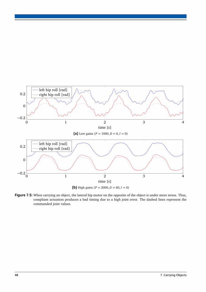
0 1 2 3 4−0.2

0

0.2

time [s]

left hip roll [rad]right hip roll [rad]

(a) Low gains (P = 1000, D = 0, I = 0)

0 1 2 3 4−0.2

0

0.2

time [s]

left hip roll [rad]right hip roll [rad]

(b) High gains (P = 2000, D = 60, I = 0)

Figure 7.5: When carrying an object, the lateral hip motor on the opposite of the object is under more stress. Thus,compliant actuation produces a bad timing due to a high joint error. The dashed lines represent thecommanded joint values.


8 Results and Experiments

In the previous chapters, we have adapted Missura’s Capture Step Framework to THOR-MANG, tunedall parameters and extended it with a hip offset to carry objects. For this purpose we had to extendthe Abstract Kinematic Interface and modify the Footstep Controller. In this chapter, we will showexperiments and evaluate how well the system performs on THOR-MANG.

8.1 Walking

After tuning the CPG as described in Section 6.3.3, THOR-MANG is able to walk open-loop both in sim-ulation and in reality. The walk is omnidirectional, i.e. the robot can walk forward, backward, sidewardand turn. When walking at a reasonable speed, we can combine all three walking dimensions withoutfalling down. We also tuned the Footstep Controller, that uses the CPG in order to stabilize the robot.We presented our methods in Section 6.3.3. When walking forward at full speed, the step size is approx-imately 0.2 m. Considering an undisturbed open-loop step frequency of 2 Hz in Simulation and 2.3 Hzin reality, the robot walks with approximately 0.4 m/s in simulation and 0.46 m/s in reality. It is actuallypossible to walk open-loop at full speed, as long as we keep the acceleration at a reasonable level. Ofcourse, a disturbance will very likely cause the robot to fall in that situation.

As long as the robot is not disturbed, the closed-loop gait does not look much different from the open-loop CPG. This is not surprising, as we tuned the Footstep Controller by fitting it to the undisturbedopen-loop gait. Thus, in order to evaluate the controller, we need to disturb the robot and observe itsmovements.Figure 8.1 shows the robot being pushed from behind in simulation. The push strength in this experimentis 200 N acting on the robot’s pelvis for 100 ms. Directly after the push, the Footstep Controller noticesthe push from the sagittal CoM velocity and the resulting wrong CoM position. The controller uses theCPG to make sagittal Capture Steps and stabilize the robot. During the recovery phase, the robot usesa much greater step size as usual, as the disturbance was very high. This shows that we have tuneda stable CPG and correctly fitted the Footstep Controller. With insufficient parameters, the Controllerwould not have been able to estimate the movements of the robot correctly. This had resulted in wrongCapture Steps that would not stabilize the robot.Figure 8.2 demonstrates that the system also works with the real robot. For safety reasons, we pulled therobot from the front instead of pushing it from behind. Again, we can see the robot making appropriateCapture Steps and compensating the disturbance.

We also conducted statistical push experiments with the simulated robot in order to show the proba-bility of a fall at different push strengths. For this chapter, we define a push to be a linear force acting onthe robot pelvis for 100 ms. We consider the robot to have successfully rejected the disturbance, if it wasstill walking after 10 s. To make the experiments statistically relevant, we had to perform a huge amountof pushes. For this purpose, we developed a Push Experimenter Tool that can be seen in Figure 8.3. Thetool provides options for the timing of the experiment, the push force and the number of repetitions. Italso provides functionality to detect simulation issues that may occur during simulation in Gazebo. Astatistical comparison between the open-loop CPG and the closed-loop Footstep Controller can be seenin Figure 8.4. In that figure, each colored square represents 50 pushes and the color shows the empiricalprobability to fall down. We can see, that the closed-loop controller stabilizes the gait as expected, whilethe open-loop robot falls more often, especially when being pushed from the side. Interestingly, we cansee in both images, that the robot is more likely to fall if it got pushed from the left. This is most likely asimulation artifact from starting the gait with the left foot.

49

(a) undisturbed (b) 0.5 s (c) 1 s (d) 1.5 s (e) 3 s

Figure 8.1: The robot can recovery from rather strong perturbations by taking Capture Steps. This shows, that theCoM reference trajectory is correct.

(a) Pulling (b) 0.5 s (c) 1 s (d) 1.5 s (e) 2.5 s

Figure 8.2: The push recovery also works with the real robot, but we cannot perform pushes as strong as insimulation without risking to damage the robot.

50 8 Results and Experiments

Figure 8.3: The custom Push Experimenter enabled us to perform the huge amount of push recovery experiments.For this this thesis, we performed 34600 pushes using that tool.

8.1 Walking 51

−150−100 −50 0 50 100 150

−150

−100

−50

0

50

100

150

Push Force X

Push

Forc

eY

0 0.2 0.4 0.6 0.8 1

(a) Open-loop

−150−100 −50 0 50 100 150

−150

−100

−50

0

50

100

150

Push Force X

0 0.2 0.4 0.6 0.8 1

(b) Closed-loop

Figure 8.4: We let the robot walk in place both in open-loop and in closed-loop mode and pushed it from differentdirections and with different strength. The colors show the empirical probability to fall determined by50 pushes per square.

8.2 Carrying Objects

During development, we simulated an additional weight by applying a vertical force on the hand of therobot. Therefore, those tests neglected any dynamical effects of the grasped object. In this section, wewill perform experiments using different objects with full dynamics. As our motivation was to carry atool, we performed experiments with a cordless drill that has a weight of 1.5 kg and a sledgehammerwith a weight of 5 kg. Additionally, the sledgehammer sticks out to the front and thus adds a largesagittal CoP offset. Figure 8.5 shows the robot with those two objects.

First, we let the robot walk in place with each grasped object and analyzed the graphs of the CoM yposition, the estimated time to step and the closed-loop gait frequency similar to our previous method.The graphs are very similar to Figure 7.4b, where we have experimented with the linear 50 N force.Thus, the dynamical objects have a very similar effect on the robot as the non-dynamical force. However,in practical situations it is not important that the graphs are looking good, but the robot shall walk stableand must reject disturbances. Therefore, we performed push experiments with the simulated robot atdifferent push-strength and with different grasped objects and compared the results with and withoutthe hip offset compensation.Figure 8.6 shows the relative frequency of falls when the robot was pushed having a drill attached tothe right hand. We performed 6600 pushes for that figure, so each bar represents 100 pushes. For thisexperiment, we let the robot walk in place for a few seconds including a random factor to average outthe effect of the current step state, before applying a push from the front or from the back. We canclearly see in Figure 8.6a, that the automatic compensation of the weight using the hip offset increasesthe stability of the gait. The figure also shows the perormance without grasped object as reference. Wecan see that the performance with the hip offset compensation is about as good as not carrying anyobject at all. When pushing the robot from the front, the hip offset does not have a noticeable effect on


(a) THOR-MANG with a drill (b) THOR-MANG with a sledgeham-mer

Figure 8.5: For experiments we attached a drill with a weight of 1.5 kg and a sledgehammer of 5 kg to the robot.The sledgehammer sticks out to the front and creates a great CoM offset in the sagittal direction.

the stability, because the drill causes a small positive sagittal CoM displacement when not compensated.This CoM displacement passively compensates pushes from the front. Moving the ground projected CoMin the middle between the feet again increases the accuracy of the Footstep Controller, but removes thepassive stability gain from the undesired CoM displacement.

When carrying a heavier object than the drill, e.g. the sledgehammer, we can see the effects moreclearly. Figure 8.7 shows the same experiment as the previous figure, but with a sledgehammer attachedto the hand. Again, each bar represents 100 pushes which sums up to a total of 4400 experiments. Wecan see that the robot always falls down when we push it from the back without compensation, becausethe hammer moves the CoP very close to the toes when standing. The robot is not able to recover frompushes in that configuration. It should be noted, that even walking in place is very difficult withoutcompensation. In this experiment, we had to move the sledgehammer to the left hand. The robot startswalking with a hip swing to the right, so attaching the hammer to the right hand causes the robot tofall over immediately. After starting to walk, the robot still walks very unstable. We always restarted theexperiment if the robot had fallen prematurely, so the figure only shows the cases when the robot wasable to walk for at least a few seconds.When pushing the robot from the front, the large CoM offset to the front helps to stabilize the robot atleast a few times, even when not actively compensating the hammer with a hip offset. We can still seein Figure 8.7b that the hip offset improves the gait stability significantly. Even when pushing from thefront, the robot will usually fall forward when not compensating the hammer.Interestingly, when comparing the results from the compensated sledgehammer in Figure 8.7a to Fig-ure 8.6a, we see that the hip offset for the hammer actually increases the gait stability compared to therobot without grasped object. There are multiple reasons that could cause that effect. Firstly, the robotbecomes heavier when carrying an object, so the acceleration is smaller when pushing with the sameforce. We might also have not perfectly tuned the CPG or the footstep controller, so the sledgehammeractually makes the robot behave more like the pendulum we have tuned and the robot’s movement bettermatches the movement estimated by the controller. Since we use a simulation, we also have to considernumerical reasons. We are using rather high D-gains for the ankles, which results in shaky feet whenever

8.2 Carrying Objects 53

150 160 170 180 190 200 210 220 230 240 2500

0.2

0.4

0.6

0.8

1

Push force X

Empi

rica

lpro

babi

lity

tofa

ll

Without any weight1.5kg cordless drill (uncompensated)1.5 kg cordless drill (compensated)

(a) Pushing from the back (positive push force)

−200 −190 −180 −170 −160 −150 −140 −130 −120 −110 −1000

0.2

0.4

0.6

0.8

1

Push force X

Empi

rica

lpro

babi

lity

tofa

ll


(b) Pushing from the front (negative push force)

Figure 8.6: This figure shows the robot walking in place with a cordless drill attached to the right hand and beingpushed with different strengths.


they are in the air. This also causes small disturbances of the support leg. The additional force from thesledgehammer makes the feet more stable when on the ground. Further testing is needed in order todetermine the actual reason for this effect, but from experience the latter reason seems to be the mostplausible.If we push the robot from the side we get similar results as in the previous experiments which can beseen in Figure 8.8 and 8.9. For these figures, the robot had the weight attached to the left hand. In Fig-ure 8.8, we can see that the uncompensated drill has a bigger impact on the lateral than on the sagittalpush recovery. This is comprehensible, as the drill does not stick out to the front or the back and thusmainly shifts the CoM to the side. The lateral motion is primarily stabilized by the step timing. With thedrill attached, the step timing becomes inaccurate and the robot is more likely to fall, when pushed fromthe side. When we push the robot from the left, we again get the result that even without compensationthe robot is still walking stable. The reason is the same as before; a weight on the left side passivelycompensates a push we apply from that direction.

We repeated the experiment with the robot walking forward and pushed it from the back. Whilewalking in place as in the previous experiments usually can be done open-loop as well, walking forwardrequires a controller to be reliable. The results can be seen in Figure 8.10. We were not able to performuncompensated tests with the sledgehammer, as the robot falls immediately when trying to walk forward.Even the drill reduces the reliability of the push recovery significantly, because the controller already hasto actively balance the robot to prevent it from falling over. When the robot does not behave as expected,the controller cannot properly track the reference trajectory and thus is not able to reject disturbanceswell. After compensating the drill, the robot walks almost as reliable as without object. We do notobserve the hammer-anomaly from Figure 8.6a and 8.7a this time, but we can see that carrying thesledgehammer is much more stable than carrying a drill without compensation.

8.3 Limits

We reached our goal of carrying objects with THOR-MANG without falling. Nevertheless, there aresome limitations to the system. The greatest limit is that the robot can only walk on flat ground. Thislimit is inherited from Missura’s Capture Step Framework, as it was only intended to work on soccerplayfields. Therefore, the robot can neither walk on slopes, nor step over objects or climb stairs. All ofthese situations might occur in a disaster scenario like in the DRC. Another limit of the Capture StepFramework is the migration effort for a different robot, as all parameters are tuned manually. We hadto retune the CPG and the Footstep Controller multiple times during this thesis, as the results were notsufficient for the next step. If we now want to modify the robot, e.g. by adding additional hardware,we would have to retune the system again. Also starting and stopping the gait with the Capture StepFramework is not trivial. While the CoM trajectory is well defined when the robot is walking, thecontroller does not model the initial and the last step. Starting the gait happens mainly open-loopby swinging the hip and raising one foot. Afterwards, we let the controller compensate the resultingdisturbance. Depending on the configuration of the robot, this initial step might already cause the robotto fall over.In addition, our hip offset calculation also assumes that the robot is standing on flat ground. When therobot stands on sloped terrain, the left and right F/T sensor will measure different weights. Thus, thecontroller will compute a wrong hip offset. We also had to add further parameters for the conversionbetween a CoP offset and the appropriate abstract kinematic hip offset. These parameters have to betuned by hand as well and thus increase the effort to use the system on another robot. At last, acompensation with a hip offset only works, if the robot has grasped an object, that can be freely movedwith respect to the feet. For instance, if the robot has grasped a railing and pushing against it, we wouldget a CoP offset away from the railing. This would cause the robot do move the hip towards the railingand eventually bring the robot to a fall.

8.3 Limits 55

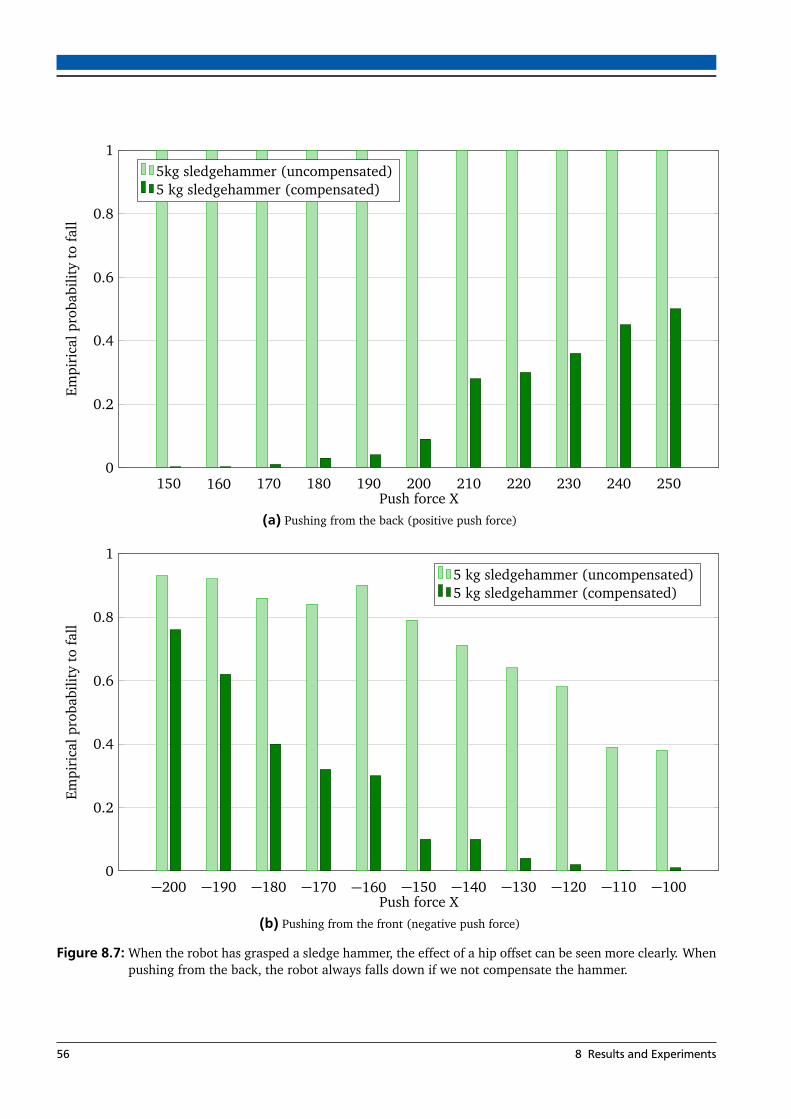
150 160 170 180 190 200 210 220 230 240 2500

0.2

0.4

0.6

0.8

1

Push force X

Empi

rica

lpro

babi

lity

tofa

ll

5kg sledgehammer (uncompensated)5 kg sledgehammer (compensated)

(a) Pushing from the back (positive push force)

−200 −190 −180 −170 −160 −150 −140 −130 −120 −110 −1000

0.2

0.4

0.6

0.8

1

Push force X

Empi

rica

lpro

babi

lity

tofa

ll

5 kg sledgehammer (uncompensated)5 kg sledgehammer (compensated)

(b) Pushing from the front (negative push force)

Figure 8.7: When the robot has grasped a sledge hammer, the effect of a hip offset can be seen more clearly. Whenpushing from the back, the robot always falls down if we not compensate the hammer.


150 160 170 180 190 200 210 220 230 240 2500

0.2

0.4

0.6

0.8

1

Push force Y

Empi

rica

lpro

babi

lity

tofa

ll


(a) Pushing from the right (positive push force)

−250 −240 −230 −220 −210 −200 −190 −180 −170 −160 −1500

0.2

0.4

0.6

0.8

1

Push force Y

Empi

rica

lpro

babi

lity

tofa

ll


(b) Pushing from the left (negative push force)

Figure 8.8: In this figure, the robot had a drill attached to the left hand and was walking in place. We pushedit from the side with different push strength. As the lateral motion is sensitive to wrong timing, theuncompensated drill has a greater effect if we push the robot from the side.

8.3 Limits 57

150 160 170 180 190 200 210 220 230 240 2500

0.2

0.4

0.6

0.8

1

Push force Y

Empi

rica

lpro

babi

lity

tofa

ll

5kg sledgehammer (uncompensated)5 kg sledgehammer (compensated)

(a) Pushing from the right (positive push force)

−250 −240 −230 −220 −210 −200 −190 −180 −170 −160 −1500

0.2

0.4

0.6

0.8

1

Push force Y

Empi

rica

lpro

babi

lity

tofa

ll

5 kg sledgehammer (uncompensated)5 kg sledgehammer (compensated)

(b) Pushing from the left (negative push force)

Figure 8.9: For this figure, the robot had a sledgehammer attached to the left hand and was walking in place. Wepushed it from the side with different push strength. As in the drill-experiment, we can see that thehip offset improves the walking stability significantly.


150 160 170 180 190 200 210 220 230 240 2500

0.2

0.4

0.6

0.8

1

Push force X

Empi

rica

lpro

babi

lity

tofa

ll


(a) Pushing while walking forward and carrying a 1.5 kg drill

150 160 170 180 190 200 210 220 230 240 2500

0.2

0.4

0.6

0.8

1

Push force X

Empi

rica

lpro

babi

lity

tofa

ll

5 kg sledgehammer (compensated)

(b) Pushing while walking forward and carrying a 5 kg sledgehammer

Figure 8.10: In this figure, we let the robot walk forward and pushed it from the back. We can see in the caseof the 1.5 kg drill, that the hip offset greatly improves the ability to recover from perturbations. Wewere not able to perform the experiment with the 5 kg hammer without compensation, as the robotwas not able to walk forward in that configuration.

8.3 Limits 59

9 Conclusion

The goal of this thesis was to get the THOR-MANG robot walking without falling while carrying a graspedobject. As developing a walking controller is a lot of work, we focused on adapting existing approaches.Our first attempt was using the Atlas Walk controller from the Drake toolbox. Drake uses a full dynamicmodel of the robot, solves a cost function with respect to a set of constraints with a QP solver andthen outputs joint torques and velocities. We adapted Drake to a level that the planning would producereasonable trajectories. With those pre-planned open-loop trajectories, THOR-MANG was able to walkin simulation. However, as converting a torque or a velocity to a joint position is a difficult task, we werenot able to get the closed-loop controller running on the position-controlled robot.Our second approach was to use Missura’s Capture Step Framework. This Framework was developedfor rather small and simple soccer robots that are usually position-controlled as well. Thus, the outputsof the walking controller are joint-positions that we can use directly. The controller stabilizes the robotusing Capture Steps; i.e. if the robot gets pushed, it takes one or multiple steps to compensate thedisturbance. We explained how we modified the Capture Step Framework for our THOR-MANG robot,but the main work was to tune the parameters. Some of those parameters are hard to obtain and haveto be tuned in a certain order. We presented our approach of tuning the CPG and the Footstep Controllerand achieved a stable open-loop gait as well as a good closed-loop disturbance rejection. The presentedapproach of tuning the parameters is also applicable for other robots.The second challenge of this thesis was to carry an object without falling down. We have met thatchallenge by compensating the CoM displacement in the horizontal plane with a hip offset. For thatpurpose, we used the F/T sensors in the ankles to obtain the CoP of the robot while standing. We thenused the CoP offset to move the hip of the robot and thus bring the ground projected CoM back inthe middle between the feet. We also had to modify the closed-loop Footstep Controller to work witha hip offset. Even though a grasped object impacts the CoM position in the horizontal plane and alsoalters the height of the CoM and the dynamical parameters of the robot, we claim that compensating theCoM offset in the horizontal plane is sufficient. We gave an exemplary calculation for a Linear InvertedPendulum Model and showed, that when the robot is carrying an object with the weight of 5 kg theangular frequency only changes by 2%.We conducted experiments with the open-loop CPG, the closed-loop Footstep Controller and differentweights to show, that our approach of tuning the parameters and compensating grasped objects works.For this purpose we performed push experiments from different directions. Our statistics show that theweight compensation with a hip offset in the horizontal plane improves the gait quality significantly.When carrying an object, the probability of a fall does not increase compared to when not carrying anyobject.

61

10 Future Work

The approach presented in this thesis enables THOR-MANG to walk, carry an object and still reject dis-turbances with Capture Steps. Of course, there is still room for improvements.While our approach requires the robot to stand still when measuring the CoP, we might also want tograb an object during walking. Thus, we could improve the system to be able to compensate the CoMoffset during a gait. By measuring the CoP of the current support foot and comparing it to the nominalZMP of the unaltered LIPM we could determine our hip offset even while walking.At the current state we think that the walking algorithm itself provides much more room for improve-ments than our weight compensation. As stated in Section 8.3, tuning the CPG and the Footstep Con-troller manually is a lot of work. Thus, one step in improving the system would be to automatize thatprocedure. If we have a detailed dynamical model of the robot, we might be able to automatically com-pute many parameters that we had to determine manually during development. For certain, we canautomatize the determination of the controller parameters, as our approach is mainly based on lettingthe robot walk open-loop and read the correct values from graphs. The goal for this step would be to im-plement a one-click-solution that starts a calibration cycle and automatically determines the parameterseither by computing them from the robot model or from automatic experiments.Additionally, our motivation was to carry a tool in a catastrophic scenario. Obviously, we cannot assumeto always have flat ground in that scenario, but Missura’s Capture Step Framework was developed forsoccer robots and cannot cope with uneven ground. The robot cannot step over objects, climb stairs oreven walk on slopes. That drawback occurred because we used a walking algorithm for a situation itwas not intended to work in. This issue needs to be fixed if we really want to apply the system in ascenario like the DRC. We could either solve that problem by extending the capabilities of the CaptureStep Framework or by choosing a different walking algorithm. Drake does not have that drawback, butas explained earlier the conversion from joint torques and velocities to joint positions did not work. Wethink that enabling the robot to walk on uneven ground and step over objects has to be next step in orderto improve the system.

63

Bibliography

[1] Sven Behnke. Online trajectory generation for omnidirectional biped walking. In Proceedings of theIEEE International Conference on Robotics and Automation (ICRA), pages 1597–1603. IEEE, 2006.

[2] Hongkai Dai, Andrés Valenzuela, and Russ Tedrake. Whole-body motion planning with centroidaldynamics and full kinematics. In IEEE-RAS 14th International Conference on Humanoid Robots(Humanoids), pages 295–302. IEEE, 2014.

[3] Andrea Del Prete, Nicolas Mansard, Oscar Efrain Ramos Ponce, Olivier Stasse, and Francesco Nori.Implementing torque control with high-ratio gear boxes and without joint-torque sensors. Interna-tional Journal of Humanoid Robotics, 2015.

[4] Johannes Englsberger, Christian Ott, Maximo Roa, Alin Albu-Schäffer, Gerhard Hirzinger, et al.Bipedal walking control based on capture point dynamics. In IEEE/RSJ International Conference onIntelligent Robots and Systems (IROS), pages 4420–4427. IEEE, 2011.

[5] Colin Graf and Thomas Röfer. A closed-loop 3d-lipm gait for the robocup standard platform leaguehumanoid. In Proceedings of the Fifth Workshop on Humanoid Soccer Robots in conjunction with the2010 IEEE-RAS International Conference on Humanoid Robots, 2010.

[6] Kensuke Harada, Shuuji Kajita, Hajime Saito, Mitsuharu Morisawa, Fumio Kanehiro, Kiyoshi Fu-jiwara, Kenji Kaneko, and Hirohisa Hirukawa. A humanoid robot carrying a heavy object. InProceedings of the IEEE International Conference on Robotics and Automation (ICRA), pages 1712–1717. IEEE, 2005.

[7] At L. Hof. The ‘extrapolated center of mass’ concept suggests a simple control of balance in walking.Human movement science, 27(1):112–125, 2008.

[8] Michael Hopkins, Dennis W Hong, Alexander Leonessa, et al. Humanoid locomotion on uneventerrain using the time-varying divergent component of motion. In IEEE-RAS 14th InternationalConference on Humanoid Robots (Humanoids), pages 266–272. IEEE, 2014.

[9] Matthew Johnson, Brandon Shrewsbury, Sylvain Bertrand, Tingfan Wu, Daniel Duran, MarshallFloyd, Peter Abeles, Douglas Stephen, Nathan Mertins, Alex Lesman, et al. Team ihmc’s lessonslearned from the darpa robotics challenge trials. Journal of Field Robotics, 32(2):192–208, 2015.

[10] Shuuji Kajita, Fumio Kanehiro, Kenji Kaneko, Kazuhito Yokoi, and Hirohisa Hirukawa. The 3dlinear inverted pendulum mode: A simple modeling for a biped walking pattern generation. InIEEE/RSJ International Conference on Intelligent Robots and Systems (IROS), pages 239–246. IEEE,2001.

[11] Shuuji Kajita, Fumio Kanehiro, Kenji Kaneko, Kiyoshi Fujiwara, Kensuke Harada, Kazuhito Yokoi,and Hirohisa Hirukawa. Biped walking pattern generation by using preview control of zero-moment point. In Proceedings of the IEEE International Conference on Robotics and Automation(ICRA), pages 1620–1626. IEEE, 2003.

[12] Shuuji Kajita, Mitsuharu Morisawa, Kensuke Harada, Kenji Kaneko, Fumio Kanehiro, Kiyoshi Fu-jiwara, and Hirohisa Hirukawa. Biped walking pattern generator allowing auxiliary zmp control.In IEEE/RSJ International Conference on Intelligent Robots and Systems (IROS), pages 2993–2999.IEEE, 2006.

65

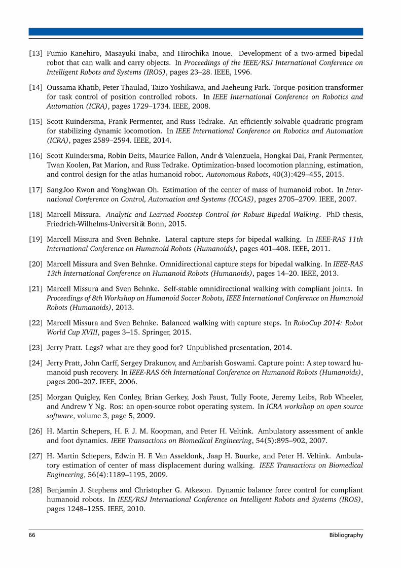
[13] Fumio Kanehiro, Masayuki Inaba, and Hirochika Inoue. Development of a two-armed bipedalrobot that can walk and carry objects. In Proceedings of the IEEE/RSJ International Conference onIntelligent Robots and Systems (IROS), pages 23–28. IEEE, 1996.

[14] Oussama Khatib, Peter Thaulad, Taizo Yoshikawa, and Jaeheung Park. Torque-position transformerfor task control of position controlled robots. In IEEE International Conference on Robotics andAutomation (ICRA), pages 1729–1734. IEEE, 2008.

[15] Scott Kuindersma, Frank Permenter, and Russ Tedrake. An efficiently solvable quadratic programfor stabilizing dynamic locomotion. In IEEE International Conference on Robotics and Automation(ICRA), pages 2589–2594. IEEE, 2014.

[16] Scott Kuindersma, Robin Deits, Maurice Fallon, Andrés Valenzuela, Hongkai Dai, Frank Permenter,Twan Koolen, Pat Marion, and Russ Tedrake. Optimization-based locomotion planning, estimation,and control design for the atlas humanoid robot. Autonomous Robots, 40(3):429–455, 2015.

[17] SangJoo Kwon and Yonghwan Oh. Estimation of the center of mass of humanoid robot. In Inter-national Conference on Control, Automation and Systems (ICCAS), pages 2705–2709. IEEE, 2007.

[18] Marcell Missura. Analytic and Learned Footstep Control for Robust Bipedal Walking. PhD thesis,Friedrich-Wilhelms-Universität Bonn, 2015.

[19] Marcell Missura and Sven Behnke. Lateral capture steps for bipedal walking. In IEEE-RAS 11thInternational Conference on Humanoid Robots (Humanoids), pages 401–408. IEEE, 2011.

[20] Marcell Missura and Sven Behnke. Omnidirectional capture steps for bipedal walking. In IEEE-RAS13th International Conference on Humanoid Robots (Humanoids), pages 14–20. IEEE, 2013.

[21] Marcell Missura and Sven Behnke. Self-stable omnidirectional walking with compliant joints. InProceedings of 8th Workshop on Humanoid Soccer Robots, IEEE International Conference on HumanoidRobots (Humanoids), 2013.

[22] Marcell Missura and Sven Behnke. Balanced walking with capture steps. In RoboCup 2014: RobotWorld Cup XVIII, pages 3–15. Springer, 2015.

[23] Jerry Pratt. Legs? what are they good for? Unpublished presentation, 2014.

[24] Jerry Pratt, John Carff, Sergey Drakunov, and Ambarish Goswami. Capture point: A step toward hu-manoid push recovery. In IEEE-RAS 6th International Conference on Humanoid Robots (Humanoids),pages 200–207. IEEE, 2006.

[25] Morgan Quigley, Ken Conley, Brian Gerkey, Josh Faust, Tully Foote, Jeremy Leibs, Rob Wheeler,and Andrew Y Ng. Ros: an open-source robot operating system. In ICRA workshop on open sourcesoftware, volume 3, page 5, 2009.

[26] H. Martin Schepers, H. F. J. M. Koopman, and Peter H. Veltink. Ambulatory assessment of ankleand foot dynamics. IEEE Transactions on Biomedical Engineering, 54(5):895–902, 2007.

[27] H. Martin Schepers, Edwin H. F. Van Asseldonk, Jaap H. Buurke, and Peter H. Veltink. Ambula-tory estimation of center of mass displacement during walking. IEEE Transactions on BiomedicalEngineering, 56(4):1189–1195, 2009.

[28] Benjamin J. Stephens and Christopher G. Atkeson. Dynamic balance force control for complianthumanoid robots. In IEEE/RSJ International Conference on Intelligent Robots and Systems (IROS),pages 1248–1255. IEEE, 2010.

66 Bibliography

[29] Eliza Strickland. 24 hours at fukushima. Spectrum, IEEE, 48(11):35–42, 2011.

[30] Russ Tedrake. Drake: A planning, control, and analysis toolbox for nonlinear dynamical systems,2014. URL http://drake.mit.edu.

[31] Miomir Vukobratovic and Branislav Borovac. Zero-moment point — thirty five years of its life.International Journal of Humanoid Robotics, 1(1):157–173, 2004.

[32] Miomir Vukobratovic and J. Stepanenko. On the stability of anthropomorphic systems. Mathemat-ical biosciences, 15(1):1–37, 1972.

[33] Pierre-Brice Wieber. Trajectory free linear model predictive control for stable walking in the pres-ence of strong perturbations. In IEEE-RAS 6th International Conference on Humanoid Robots (Hu-manoids), pages 137–142. IEEE, 2006.

[34] X Xinjilefu, Siyuan Feng, and Christopher G. Atkeson. Center of mass estimator for humanoidsand its application in modelling error compensation, fall detection and prevention. IEEE-RAS 15thInternational Conference on Humanoid Robots (Humanoids), 2015.

[35] Seung-Joon Yi, Byoung-Tak Zhang, Dennis Hong, and Daniel D. Lee. Practical bipedal walkingcontrol on uneven terrain using surface learning and push recovery. In IEEE/RSJ InternationalConference on Intelligent Robots and Systems (IROS), pages 3963–3968. IEEE, 2011.

[36] Seung-Joon Yi, Stephen G. McGill, Byoung-Tak Zhang, Do-Kwan Hong, and Daniel D. Lee. Activestabilization of a humanoid robot for real-time imitation of a human operator. In IEEE-RAS 12thInternational Conference on Humanoid Robots (Humanoids), pages 761–766. IEEE, 2012.

[37] Seung-Joon Yi, Stephen McGill, Larry Vadakedathu, Qin He, Inyong Ha, Jeakwon Han, HyunjongSong, Michael Rouleau, Dennis Hong, and Daniel D. Lee. Thor-op humanoid robot for darparobotics challenge trials 2013. In IEEE 11th International Conference on Ubiquitous Robots andAmbient Intelligence (URAI), pages 359–363. IEEE, 2014.

[38] Seung-Joon Yi, Stephen McGill, Larry Vadakedathu, Qin He, Inyong Ha, Michael Rouleau, Do-KwanHong, and Daniel D. Lee. Modular low-cost humanoid platform for disaster response. In IEEE/RSJInternational Conference on Intelligent Robots and Systems (IROS), pages 965–972. IEEE, 2014.

Bibliography 67

http://drake.mit.edu

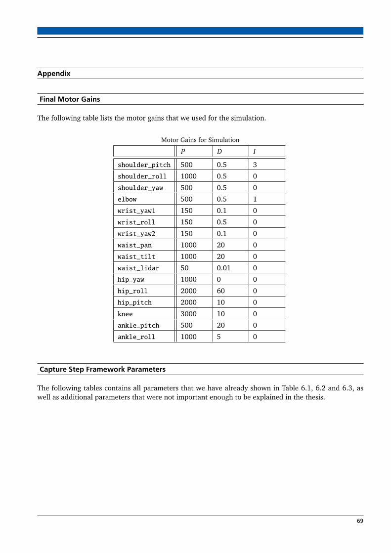
Appendix

Final Motor Gains

The following table lists the motor gains that we used for the simulation.

Motor Gains for Simulation

P D I

shoulder_pitch 500 0.5 3

shoulder_roll 1000 0.5 0

shoulder_yaw 500 0.5 0

elbow 500 0.5 1

wrist_yaw1 150 0.1 0

wrist_roll 150 0.5 0

wrist_yaw2 150 0.1 0

waist_pan 1000 20 0

waist_tilt 1000 20 0

waist_lidar 50 0.01 0

hip_yaw 1000 0 0

hip_roll 2000 60 0

hip_pitch 2000 10 0

knee 3000 10 0

ankle_pitch 500 20 0

ankle_roll 1000 5 0

Capture Step Framework Parameters

The following tables contains all parameters that we have already shown in Table 6.1, 6.2 and 6.3, aswell as additional parameters that were not important enough to be explained in the thesis.

69

Halt Position


armAngleX 0.35 0.35

armAngleY 0 0

armExtension 0.1 0.1

legAngleX 0.11 0.11

legAngleY -0.06 -0.02

torsoAngleY 0.18 0.2

legExtension 0.05 0.05

footAngleX 0 0

footAngleY 0 0

70 Appendix

CPG Parameters


gaitFrequency 2 2.3

gaitFrequencySlopeY 0 0

gaitFrequencySlopeX 0 0

firstStepDuration 0.3 0.3

firstStepHipSwing 0.3 0.3

stoppingVelocity 1 1

swingStartTiming 0.39 0.39

swingStopTiming 2.3876 2.3876

liftStartTiming 0 0

liftStopTiming 3.14159 3.14159

pushHeight 0 -0.01

pushHeightSlope 0 0

stepHeight 0.1 0.1

stepHeightSlopeX 0.05 0

stepHeightSlopeY 0 0

virtualSlope 0.01 0.02

armSwing 0 0

armSwingSlope 0 0

stepLengthYSlope 0.08 0.08

stepLengthXPushout 0 0

stepLengthYPushout 0 0

stepLengthZPushout 0 0

stepLengthZSlope 0.2 0.2

stepLengthZVPushout 0 0

stepLengthXSlopeFwd 0.2 0.2

stepLengthXSlopeBwd 0.2 0.2

lateralHipSwing 0.096 0.132

lateralHipSwingSlope 0 0

tiltSpeedFwd 0 0

tiltSpeedBwd 0 0

tiltRotLean 0 0

71

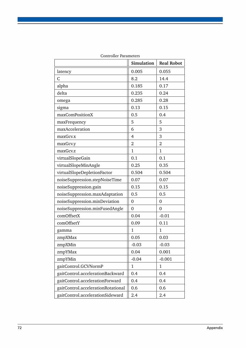
Controller Parameters


latency 0.005 0.055

C 8.2 14.4

alpha 0.185 0.17

delta 0.235 0.24

omega 0.285 0.28

sigma 0.13 0.15

maxComPositionX 0.5 0.4

maxFrequency 5 5

maxAcceleration 6 3

maxGcv.x 4 3

maxGcv.y 2 2

maxGcv.z 1 1

virtualSlopeGain 0.1 0.1

virtualSlopeMinAngle 0.25 0.35

virtualSlopeDepletionFactor 0.504 0.504

noiseSuppression.stepNoiseTime 0.07 0.07

noiseSuppression.gain 0.15 0.15

noiseSuppression.maxAdaptation 0.5 0.5

noiseSuppression.minDeviation 0 0

noiseSuppression.minFusedAngle 0 0

comOffsetX 0.04 -0.01

comOffsetY 0.09 0.11

gamma 1 1

zmpXMax 0.05 0.03

zmpXMin -0.03 -0.03

zmpYMax 0.04 0.001

zmpYMin -0.04 -0.001

gaitControl.GCVNormP 1 1

gaitControl.accelerationBackward 0.4 0.4

gaitControl.accelerationForward 0.4 0.4

gaitControl.accelerationRotational 0.6 0.6

gaitControl.accelerationSideward 2.4 2.4

72 Appendix

Hip Offset Parameters

Simulation

hipOffsetXRatio 1.06

hipOffsetYRatio 1.9

minHipOffsetX -0.2

maxHipOffsetX 0.2

minHipOffsetY -0.2

maxHipOffsetY 0.2

adaptationPerSecond 0.05

73

Robust Locomotion of a Humanoid Robot Considering Grasped ... · In this thesis, we investigate an...

Documents

Transcript of Robust Locomotion of a Humanoid Robot Considering Grasped ... · In this thesis, we investigate an...