Strömung um NACA-Profile mit einer Panelmethode Lösungen

Strömung um NACA-Profilemit einer Panelmethode

Lösungen

Fakultät Maschinenwesen Institut für Luft- und Raumfahrrtechnik

Übung Aerodynamik 2, Sommersemester 2008Thomas Albrecht

TU Dresden, 15.07.08 Strömung um NACA-Profile Folie 2

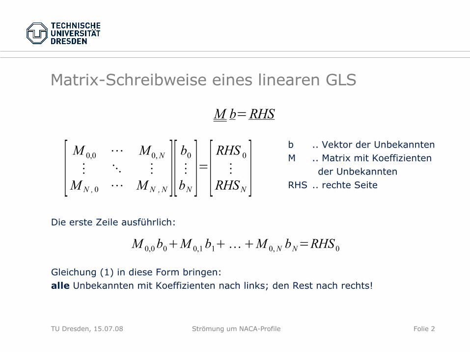
Matrix-Schreibweise eines linearen GLS

M b=RHS

Die erste Zeile ausführlich:

[M 0,0 ⋯ M 0,N

⋮ ⋱ ⋮

M N , 0 ⋯ M N ,N][b0⋮

bN ]=[RHS 0⋮

RHSN ]

Gleichung (1) in diese Form bringen: alle Unbekannten mit Koeffizienten nach links; den Rest nach rechts!

M 0,0b0M 0,1b1M 0,N bN=RHS0

b .. Vektor der UnbekanntenM .. Matrix mit Koeffizienten

der UnbekanntenRHS .. rechte Seite


Matrix-Schreibweise eines linearen GLS

In Matrix-Schreibweise:

[A0,0 ⋯ A0,N −1 −1⋮ ⋱ ⋮ −1AN , 0 ⋯ AN−1,N−1 −11 0 1 0

] [0⋮

N−1

C]= [

−U∞ y0V ∞ x0⋮

−U ∞ y N−1V ∞ x N−1

0]

A0,00A0,11A0,N−1N−1−1⋅C =−U ∞ y iV ∞ x i

x i , y i = U∞ y i−V ∞ x i∑ j=0

N −1 j Aij= C

Bsp. für i = 0 und die Kutta-Bedingung. Alle Unbekannten links, der Rest rechts:

1⋅001⋅N−10 = 0

0 =−N−1


Matrix-Assemblierung in panel.py# -- allocate storage for matrixM = zeros((N+1,N+1), float64) for i in range(0,N): for j in range(0,N): if i == j: M[i][i] = compute_Aii(xl[j],yl[j],xr[j],yr[j]) else: M[i][j] = compute_Aij(xc[i],yc[i],xl[j],yl[j],xr[j],yr[j])

# -- coefficients of Cfor i in range(0,N): M[i][N] = 1.

# -- Kutta conditionM[N][0] = 1.M[N][N1] = 1.

(xl, yl) .. linke und (xr, yr) .. rechte Endpunkte der Panel (xc, yc) .. Kontrollpunkte

<= Matrix hat Dimension N+1 × N+1,initialisiert mit Nullen

<= Schleife läuft von 0 bis N-1


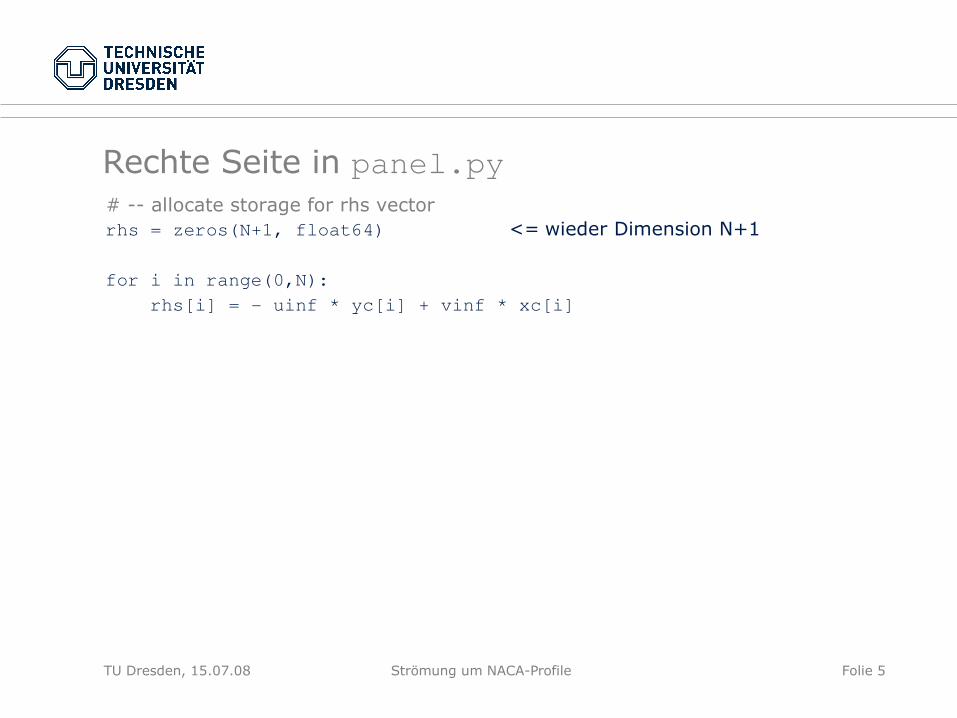
Rechte Seite in panel.py# -- allocate storage for rhs vectorrhs = zeros(N+1, float64)

for i in range(0,N): rhs[i] = uinf * yc[i] + vinf * xc[i]

<= wieder Dimension N+1


Umströmung NACA 0015

• panel.py ausführenaero2@mlr033 ~> ./panel.py

• Vektoren plottengnuplot> scale=0.1gnuplot> plot „vectors.dat“ u 1:2:($3*scale):($4*scale) w vec

• Stromlinien plottenaero2@mlr033 ~> gnuplot streamf.gp


Umströmung NACA 0015 bei 0°


Umströmung NACA 0015 bei 5°


Umströmung NACA 66(215)-216 bei 1.04°


Druckbeiwert

c p x =px − p∞q∞

2U ∞2 p∞ =

2U2

x p x

c p x = 1−U x U ∞

2

.

Mit der Definition des Druckbeiwertes

und Bernoulli

wird

U∞ und U sind jeweils die Geschwindigkeitsbeträge!


Druckbeiwert in panel.py

for i in range(0, N):

# -- evaluate velocity at the control point i (?) x = xc[i] y = yc[i] w = complex_vel(x, y) u = w.real v = w.imag umag = math.sqrt(u**2 + v**2) cp = 1. (umag/U)**2.0

# -- write data to file f.write("%f %f %f %f %f\n" % (x,y, cp, u,v))

Problem: in den Kontrollpunkten ist die Geschwindigkeit singulär!Lösung: neben den Kontrollpunkten rechnen

<= berechnet komplexe Geschwindigkeit am Punkt (x, y)


Druckbeiwert in panel.py

for i in range(0, N):

# -- evaluate velocity near control point i

# we need the panel normal vector (nx, ny)T

dx = xr[i] xl[i] dy = yr[i] yl[i] l = math.sqrt(dx**2 + dy**2) nx = dy / l ny = dx / l

x = xc[i] + 0.01 * nx y = yc[i] + 0.01 * ny w = complex_vel(x, y) ...

<= wir rechnen ein Stückchen (in Normalenrichtung) ausserhalb der Profiloberfläche


Druckverteilung NACA 0015 bei 0°

Experimentelle Daten in naca0015pressure.dat (aus NACA-TR 824, S. 71)


Druckverteilung NACA 66(215)-216 bei 1.04°

Experimentelle Daten in naca66(215)216pressure.dat (NACA-TR 824, S. 11)


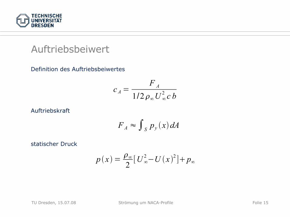
Auftriebsbeiwert

c A=F A

1/2∞U ∞2 c b

F A ≈∫Spy xdA

Definition des Auftriebsbeiwertes

Auftriebskraft

statischer Druck

p x =∞

2[U ∞

2−U x 2]p∞


Auftriebsbeiwert in panel.py

Fx = Fy = 0for i in range(0, N):

# -- evaluate velocity near control point i

# we need the panel normal vector (nx, ny)T

... p = 0.5 * (U**2 – umag**2) Fx += nx * p * l Fy += ny * p * l

# -- Lift is perpendicular to the free stream velocity vectorFl = Fy * cos(alpha) Fx * sin(alpha)print "Lift coefficient c_l = ", Fl / (0.5 * U**2)

Für NACA 66(215)-216 bei 1.04°:Experiment c

A = 0.23

panel.py cA = 0.29

<= Normalenvektor, Panellänge und Geschwindigkeitsbetrag haben wir schon (von c

P)

Strömung um NACA-Profile mit einer Panelmethode Lösungen

Documents

Transcript of Strömung um NACA-Profile mit einer Panelmethode Lösungen