Week 7 Riemann Stieltjes Integration: Lectures 19-21
24
Week 7 Riemann Stieltjes Integration: Lectures 19-21 Lecture 19 Throughout this section α will denote a monotonically increasing func- tion on an interval [a, b]. Let f be a bounded function on [a, b]. Let P = {a = a 0 <a 1 , ··· ,a n = b} be a partition of [a, b]. Put Δα i = α(a i ) - α(a i-1 ). M i = sup{f (x): a i-1 ≤ x ≤ a i }. m i = inf {f (x): a i-1 ≤ x ≤ a i }. U (P, f )= n X i=1 M i Δα i ; L(P, f )= n X i=1 m i Δα i . ¯ Z b a fdα = inf {U (P, f ): P }; Z b a fdα = sup{L(P, f ): P }. Definition 1 If ¯ Z b a fdα = Z b a fdα, then we say f is Riemann-Stieltjes (R-S) integrable w.r.t. to α and denote this common value by Z b a fdα := Z b a f (x)dα(x) := ¯ Z b a fdα = Z b a fdα. 0
Transcript of Week 7 Riemann Stieltjes Integration: Lectures 19-21

Week 7 Riemann Stieltjes
Integration:
Lectures 19-21
Lecture 19
Throughout this section α will denote a monotonically increasing func-
tion on an interval [a, b].
Let f be a bounded function on [a, b].
Let P = {a = a0 < a1, · · · , an = b} be a partition of [a, b]. Put
∆αi = α(ai)− α(ai−1).
Mi = sup{f(x) : ai−1 ≤ x ≤ ai}.mi = inf{f(x) : ai−1 ≤ x ≤ ai}.
U(P, f) =n∑i=1
Mi∆αi; L(P, f) =n∑i=1
mi∆αi.∫̄ b
a
fdα = inf{U(P, f) : P};∫ b
a
fdα = sup{L(P, f) : P}.
Definition 1 If
∫̄ b
a
fdα =
∫ b
a
fdα, then we say f is Riemann-Stieltjes
(R-S) integrable w.r.t. to α and denote this common value by∫ b
a
fdα :=
∫ b
a
f(x)dα(x) :=
∫̄ b
a
fdα =
∫ b
a
fdα.
0

Let R(α) denote the class of all R-S integrable functions on [a, b].
Definition 2 A partition P ′ of [a, b] is called a refinement of another
partition P of [a, b] if, points of P are all present in P ′. We then write
P ≤ P ′.
Lemma 1 If P ≤ P ′ then L(P ) ≤ L(P ′) and U(P ) ≥ U(P ′).
Enough to do this under the assumption that P ′ has one extra point
than P. And then it is obvious because if a < b < c then
inf{f(x) : a ≤ x ≤ c} ≤ min{inf{f(x) : a ≤ x ≤ b}, inf{f(x) : b ≤ x ≤ c}
etc.
Theorem 1
∫̄ b
a
fdα ≥∫ b
a
fdα.
For first of all, because for every partition P we have U(P, f) ≥ L(P, f).
Let P and Q be any two partitions of [a, b]. By taking a common
refinement T = P ∪Q, and applying the above lemma we get
U(P ; f) ≥ U(T ; f) ≥ L(T ; f) ≥ L(Q; f)
Now varying Q over all possible partitions and taking the supremum,
we get
U(P ) ≥∫ b
a
fdα.
Now varying P over all partitions of [a, b] and taking the infimum, we
get the theorem. ♠
Theorem 2 Let f be a bounded function and α be a monotonically
increasing function. Then the following are equivalent.
(i) f ∈ R(α).
(ii) Given ε > 0, there exists a partition P of [a, b] such that
U(P, f)− L(P, f) < ε.
1

(iii) Given ε > 0, there exists a partition P of [a, b] such that for all
refinements of Q of P we have
U(Q, f)− L(Q, f) < ε.
(iv) Given ε > 0, there exists a partition P = {a0 < a1 < cdots < an}of [a, b] such that for arbitrary points ti, si ∈ [ai−1, ai] we have
n∑i=1
|f(si)− f(ti)|∆αi < ε.
(v) There exists a real number η such that for every ε > 0, there exists
a partition P = {a0 < a1, < · · · < an} of [a, b] such that for arbitrary
points ti ∈ [ai−1, ai], we have |∑n
i=1 f(ti)∆αi − η| < ε.
Proof: (i) =⇒ (ii): By definition of the upper and lower integrals,
there exist partitions Q, T such that
U(Q)−∫̄ b
a
fdα < ε/2;
∫ b
a
fdα− L(T ) < ε/2.
Take a common refinement P to Q and T and replace Q, T by P in
the above inequalities, and then add the two inequalities and use the
hypothesis (i) to conclude (ii).
(ii) =⇒ (i): Since L(P ) ≤∫ bafdα ≤
∫̄ bafdα ≤ U(P ) the conclusion
follows.
(ii) =⇒ (iii): This follows from the previous theorem for if P ′ ≥ P then
L(P ) ≤ L(P ′) ≤ U(P ′) ≤ U(P ).
(iii) =⇒ (ii): Obvious.
(iii) =⇒ (iv): Note that |f(si)− f(ti)| ≤Mi −mi. Therefore,∑i
|f(si)− f(ti)|∆αi ≤∑i
(Mi −mi)∆αi = U(P, f)− L(P, f) < ε.
2

(iv) =⇒ (iii): Choose points ti, si ∈ [ai−1, ai] such that
|mi − f(si)| <ε
2n∆αi, |Mi − f(ti)| <
ε
2n∆αi.
Then U(P, f)− L(P, f)−∑
i(Mi −mi)∆αi
≤∑
i[|Mi − f(ti)|+ |mi − f(si)|+ |f(ti)− f(si)]∆αi < 2ε.
Thus so far, we have proved that (i) to (iv) are all equivalent to each
other.
(i) =⇒ (v): We first note that having proved that (i) to (iv) are all
equivalent, we can use any one of them. We take η =∫ bafdα. Given
ε > 0 we choose a partition P such that |L(P ) − η| < ε/3. and a
partition Q such that (iv) holds with ε replaced by ε/3. We then take a
common refinement T of these two partitions for which again the same
would hold because of (iii). We now choose si ∈ [ai−1, ai] such that
|mi − f(si)| < ε3n∆αi
whenever ∆αi is non zero. (If ∆αi = 0 we can
take si to be any point.) Then for arbitrary points ti ∈ [ai−1, ai], we
have
|∑
i f(ti)∆αi − η|
=
∣∣∣∣∣∑i
[(f(ti)− f(si) + (f(si)−mi) +mi]∆αi − η
∣∣∣∣∣≤
∑i
|f(si)− f(ti)|∆αi +∑i
|f(si)−mi|∆αi + |L(P )− η|
≤ ε/3 + ε/3 + ε/3 = ε.
(v) =⇒ (iv): Given ε > 0 choose a partition as in (v) with ε replaced
by ε/2. ♠
3

Lecture 20
Fundamental Properties of the Riemann-Stieltjes Integral
Theorem 3 Let f, g be bounded functions and α be an increasing func-
tion on an interval [a, b].
(a) Linearity in f : This just means that if f, g ∈ R(α), λ, µ ∈ R then
λf + µg ∈ R(α). Moreover,∫ b
a
(λf + µg) = λ
∫ b
a
fdα + µ
∫ b
a
fdα.
(b) Semi-Linearity in α. This just means if f ∈ R(αj), j = 1, 2 λj > 0
then f ∈ R(λ1α1 + λ2α2) and moreover,∫ b
a
fd(λ1α1 + λ2α2) = λ
∫ b
a
fdα1 + µ
∫ b
a
fdα2.
(c) Let a < c < b. Then f ∈ R(α) on [a, b] if f ∈ R(α) on [a, c] as well
as on [c, b]. Moreover we have∫ b
a
fdα =
∫ c
a
fdα +
∫ b
c
fdα.
(d) f1 ≤ f2 on [a, b] and fi ∈ R(α) then∫ baf1dα ≤
∫ baf2dα.
(e) If f ∈ R(α) and |f(x)| ≤M then∣∣∣∣∫ b
a
fdα
∣∣∣∣ ≤M [α(b)− α(a)].
(f) If f is continuous on [a, b] then f ∈ R(α).
(g) f : [a, b] → [c, d] is in R(α) and φ : [c, d] → R is continuous then
φ ◦ f ∈ R(α).
(h) If f ∈ R(α) then f 2 ∈ R(α).
(i) If, f, g ∈ R(α) then fg ∈ R(α).
(j) If f ∈ R(α) then |f | ∈ R(α) and∣∣∣∣∫ b
a
fdα
∣∣∣∣ ≤ ∫ b
a
|f |dα.
4

Proof: (a) Put h = f + g. Given ε > 0, choose partitions P,Q of [a, b]
such that
U(P, f)− L(P, f) < ε/2, P (Q, g)− L(Q, g) < ε/2
and replace these partitions by their common refinement T and then
appeal to
L(T, f) + L(T, g) ≤ L(T, h) ≤ U(T, h) ≤ U(T, f) + U(T, g).
For a constant λ since
U(P, λf) = λU(P, f); L(P, λf) = λL(P.f)
it follows that
∫ b
a
λfdα = λ
∫ b
a
fdα. Combining these two we get the
proof of (a).
(b) This is easier: In any partition P we have
∆(λ1α1 + λ2α2) = λ1∆α1 + λ2∆α2
from which the conclusion follows.
(c) All that we do is to stick to those partitions of [a, b] which contain
the point c.
(d) This is easy and
(e) is a consequence of (d).
(f) Given ε > 0, put ε1 = εα(b)−α(a)
. Then by uniform continuity of f,
there exists a δ > 0 such that |f(t) − f(s)| < ε1 whenever t, s ∈ [a, b]
and |t− s| < δ. Choose a partition P such that ∆αi < δ for all i. Then
it follows that Mi −mi < ε1 and hence U(P )− L(P ) < ε.
(g) Given ε > 0 by uniform continuity of φ, we get ε > δ > 0 such that
|φ(t)−φ(s)| < ε for all t, s ∈ [c, d] with |t− s| < δ. There is a partition
P of [a, b] such that
U(P, f)− L(P, f) < δ2.
5
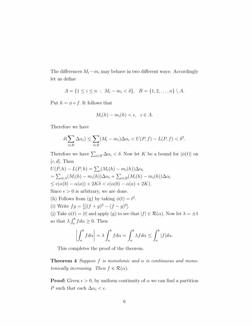
The differences Mi−mi may behave in two different ways: Accordingly
let us define
A = {1 ≤ i ≤ n : Mi −mi < δ}, B = {1, 2, . . . , n} \ A.
Put h = φ ◦ f. It follows that
Mi(h)−mi(h) < ε, i ∈ A.
Therefore we have
δ(∑i∈B
∆αi) ≤∑i∈B
(Mi −mi)∆αi < U(P, f)− L(P, f) < δ2.
Therefore we have∑
i∈B ∆αi < δ. Now let K be a bound for |φ(t)| on
[c, d]. Then
U(P, h)− L(P, h) =∑
i(Mi(h)−mi(h))∆αi
=∑
i∈A(Mi(h)−mi(h))∆αi +∑
i∈B(Mi(h)−mi(h))∆αi
≤ ε(α(b)− α(a)) + 2Kδ < ε(α(b)− α(a) + 2K).
Since ε > 0 is arbitrary, we are done.
(h) Follows from (g) by taking φ(t) = t2.
(i) Write fg = 14[(f + g)2 − (f − g)2].
(j) Take φ(t) = |t| and apply (g) to see that |f | ∈ R(α). Now let λ = ±1
so that λ∫ bafdα ≥ 0. Then∣∣∣∣∫ b
a
fdα
∣∣∣∣ = λ
∫ b
a
fdα =
∫ b
a
λfdα ≤∫ b
a
|f |dα.
This completes the proof of the theorem.
Theorem 4 Suppose f is monotonic and α is continuous and mono-
tonically increasing. Then f ∈ R(α).
Proof: Given ε > 0, by uniform continuity of α we can find a partition
P such that each ∆αi < ε.
6

Now if f is increasing, then we have Mi = f(ai),mi = f(ai−1).
Therefore,
U(P )− L(P ) =∑i
[f(ai)− f(ai−1)]∆αi < f(b)− f(a))ε.
Since ε > 0 is arbitrary, we are done. ♠
Lecture 21
Theorem 5 Let f be a bounded function on [a, b] with finitely many
discontinuities. Suppose α is continuous at every point where f is dis-
continuous. Then f ∈ R(α).
Proof: Because of (c) of theorem 3, it is enough to prove this for the
case when c ∈ [a, b] is the only discontinuity of f. Put K = sup|f(t)|.Given ε > 0, we can find δ1 > 0 such that α(c + δ1) − α(c − δ1) < ε.
By uniform continuity of f on [a, b] \ (c − δ, c + δ) we can find δ2 > 0
such that |x − y| < δ2 implies |f(x) − f(y)| < ε. Given any partition
P of [a, b] choose a partition Q which contains the points c and whose
‘mesh’ is less than min{δ1, δ2}. It follows that U(Q)−L(Q) < ε(α(b)−α(a)) + 2Kε. Since ε > 0 is arbitrary this implies f ∈ R(α). ♠
Remark 1 The above result leads one to the following question. As-
suming that α is continuous on the whole of [a, b], how large can be
the set of discontinuities of a function f such that f ∈ R(α)? The an-
swer is not within R-S theory. Lebesgue has to invent a new powerful
theory which not only answers this and several such questions raised
by Riemann integration theory but also provides a sound foundation
to the theory of probability.
Example 1 We shall denote the unit step function at 0 by U which
7

is defined as follows:
U(x) =
{0, x ≤ 0;
1, x > 0.
By shifting the origin at other points we can get other unit step func-
tion. For example, suppose c ∈ [a, b]. Consider α(x) = U(x − c), x ∈[a, b]. For any bounded function f : [a, b] → R, let us try to compute∫ bafdα. Consider any partition P of [a, b] in which c = ak. The only
non zero ∆αi is ∆αk = 1. Therefore U(P )− L(P ) = Mk(f)−mk(f).
Now assume that f is continuous at c. Then by choosing ak+1 close
to ak = c, we can make Mk − mk → 0. This means that f ∈ R(α).
Indeed, it follows that Mk → f(c) and mk → f(c). Therefore,∫ b
a
fdα = f(c).
Now suppose f has a discontinuity at c of the first kind i.e, in
particular, f(c+) exists. It then follows that |Mk−mk| → |f(c)−f(c+)|.Therefore, f ∈ R(α) iff f(c+) = f(c).
Thus, we see that it is possible to destroy integrability by just dis-
turbing the value of the function at one single point where α itself is
discontinuous.
In particular, take f = α. It follows that α 6∈ R(α) on [a, b].
We shall now prove a partial converse to (c) of Theorem 3.
Theorem 6 Let f be a bounded function and α an increasing function
on [a, b]. Let c ∈ [a, b] at which (at least) f or α is continuous. If
f ∈ R(α) on [a, b] then f ∈ R(α) on both [a, c] and [c, b]; moreover, in
that case, ∫ b
a
fdα =
∫ c
a
fdα +
∫ b
c
fdα.
8

Proof: Assume α is continuous at c. If Tc is the translation function
Tc(x) = x − c then the functions g1 = U ◦ T and g2 = 1 − U ◦ Tare both in R(α) since they are discontinuous only at c. Therefore
fg1, fg2 ∈ R(α). But these respectively imply that f ∈ R(α) on [c, b]
and on [a, c].
We now consider the case when f is continuous at c. We shall prove
that f ∈ R(α) on [a, c], the proof that f ∈ R(α) on [c, b] being similar.
Recall that the set of discontinuities of a monotonic function is
countable. Therefore there exist a sequence of points cn in [a, c] (we
are assuming that a < c) such that cn → c. By the earlier case f ∈ R(α)
on each of the intervals [a, cn]. We claim that the sequence
sn :=
∫ cn
a
fdα
converges to a limit which is equal to∫ cafdα. Let K > 0 be a bound
for α. Given ε > 0 we can choose δ > 0 such that for x, y ∈ [c− δ, c +
δ], |f(x) − f(y)| < ε/2K. If n0 is big enough then n,m ≥ n0 implies
that |sn − sm| < ε. This means {sn} Cauchy and hence is convergent
with limit equal to say, s. Now choose n so that |s− sn| < ε.
Put ∆ = α(c) − α(c−). Since cn → c, from the left, it follows that
α(cn)→ α(c−). Choose n large enough so that
|α(cn)− α(c−)| < ε/L
where L is a bound for f.
Now, choose any partition Q of [a, cn] so that |U(Q, f) − sn| < ε.
This is possible because f ∈ R(α) on [a, cn]. Put P = Q ∪ {c}, M =
max{f(x) : x ∈ [cn, c]}. Then
|s+ ∆f(c)− U(P, f)|≤ |s− sn|+ |sn − U(Q, f)|+ |∆f(c)− (α(c)− α(cn))M |≤ ε+ ε+ |∆(f(c)−M)|+ |(α(cn)− α(c−))M |≤ 2ε+ ∆ ε
2K+ |M | ε
K≤ 4ε.
9

Theorem 7 Let {cn} be a sequence of non negative real numbers such
that∑
n cn < ∞. Let tn ∈ (a, b) be a sequence of distinct points in
the open interval and let α =∑
n cnU ◦ T−tn . Then for any continuous
function f on [a, b] we have∫ b
a
fdα =∑n
cnf(tn).
Proof: Observe that for any x ∈ [a, b], 0 ≤∑
n U(x− tn) ≤∑
n cn and
hence α(x) makes sense. Also clearly it is monotonically increasing
and α(a) = 0 and α(b) =∑
n cn. Given ε > 0 choose n0 such that∑n>n0
cn < ε. Take
α1 =∑n≤n0
U ◦ T−tn , α2 =∑n>n0
U ◦ T−tn .
By (b) of theorem 3, and from the example above, we have∫ b
a
fdα1 =∑n≤n0
cnf(tn).
If K is bound for |f | on [a, b] we also have∣∣∣∣∫ b
a
fdα2
∣∣∣∣ < K(α2(b)− α2(a)) = K∑n>n0
cn = Mε.
Therefore, ∣∣∣∣∣∫ b
a
fdα−∑n≤n0
cnf(tn)
∣∣∣∣∣ < Kε.
This proves the claim. ♠
Theorem 8 Let α be an increasing function and α′ ∈ R(x) on [a, b].
Then for any bounded real function on [a, b], f ∈ R(α) iff fα′ ∈ R(x).
Furthermore, in this case,∫ b
a
fdα =
∫ b
a
f(x)α′(x)dx.
10
Proof: Given ε > 0, since α′ is Riemann integrable, by (iv) of theorem
2, there exists a partition P = {a = a0 < a1 < · · · < an = b} of [a, b]
such that for all si, ti ∈ [ai−1, ai] we have,
n∑i=1
|α′(si)− α′(ti)|∆xi < ε.
Apply MTV to α to obtain ti ∈ [ai−1, ai] such that ∆αi = α′(ti)∆xi.
Put M = sup|f(x)|. Then
n∑i=1
f(si)∆αi =n∑i=1
f(si)α′(ti)∆xi.
Therefore,∣∣∣∣∣n∑i=1
f(si)∆xi −n∑i=1
f(si)α′(si)∆xi
∣∣∣∣∣ <∑i
|f(si)||α′(si)−α′(ti)|∆xi > Mε.
Therefore
n∑i=1
f(si)∆xi ≤n∑i=1
f(si)α′(si)∆xi +Mε ≤ U(P, fα′) +Mε.
Since this is true for arbitrary si ∈ [ai−1, ai], it follows that
U(P, f, α) ≤ U(P, fα′) +Mε.
Likewise, we also obtain
U(P, fα′) ≤ U(P, f, α)) +Mε.
Thus
|U(P, f, α)− U(P, fα′)| < Mε.
Exactly in the same manner, we also get
|L(P, f, α−L(P, fα′)| < Mε.
11

Note that the above two inequalities hold for refinements of P as well.
Now suppose f ∈ R(α). we can then assume that the partition P is
chosen so that
|U(P, f, α)− L(P, fα)| < Mε.
It then follows that
|U(P, fα′)− L(P, fα′)| < 3Mε.
Since ε > 0 is arbitrary, this implies fα′ is Riemann integrable. The
other way implication is similar. Moreover, the above inequalities also
establish the last part of the theorem. ♠
Remark 2 The above theorems illustrate the power of Stieltjes’ modi-
fication of Riemann theory. In the first case, α was a staircase function
(also called a pure step function). The integral therein is reduced to
a finite or infinite sum. In the latter case, α is a differentiable func-
tion and the integral reduced to the ordinary Riemann integral. Thus
the R-S theory brings brings unification of the discrete case with the
continuous case, so that we can treat both of them in one go. As an
illustrative example, consider a thin straight wire of finite length. The
moment of inertia about an axis perpendicular to the wire and through
an end point is given by ∫ l
0
x2dm
where m(x) denotes the mass of the segment [0, x] of the wire. If
the mass is given by a density function ρ, then m(x) =∫ x
0ρ(t)dt or
equivalently, dm = ρ(x)dx and the moment of inertia takes form∫ l
0
x2ρ(x)dx.
On the other hand if the mass is made of finitely many values mi
12

concentrated at points xi then the inertia takes the form∑i
x2imi.
Theorem 9 Change of Variable formula Let φ : [a, b]→ [c, d] be a
strictly increasing differentiable function such that φ(a) = c, φ(b) = d.
Let α be an increasing function on [c, d] and f be a bounded function
on [c, d] such that f ∈ R(α). Put β = α ◦ φ, g = f ◦ φ. Then g ∈ R(β)
and we have ∫ b
a
gdβ =
∫ d
c
fdα.
Proof: Since φ is strictly increasing, it defines a one-one correspon-
dence of partitions of [a, b] with those of [c, d], given by
{a = a0 < a1 < · · · < an = b} ↔ {c = φ(a) < φ(a1) < · · · < φ(an) = d}.
Under this correspondence observe that the value of the two functions
f, g are the same and also the value of function α, β are also the same.
Therefore, the two upper sums lower sums are the same and hence the
two upper and lower integrals are the same. The result follows. ♠
13

Week 8 Functions of
Bounded Variation Lectures
22-24
Lecture 22 : Functions of bounded Variation
Definition 3 Let f : [a, b] → R be any function. For each partition
P = {a = a0 < a1 < · · · < an = b} of [a, b], consider the variations
V (P, f) =n∑k=1
|f(ak)− f(ak−1)|.
Let
Vf = Vf [a, b] = sup{V (P, f) : P is a partition of [a, b]}.
If Vf is finite we say f is of bounded variation on [a, b]. Then Vf is
called the total variation of f on [a, b]. Let us denote the space of all
functions of bounded variations on [a, b] by BV [a, b].
Lemma 2 If Q is a refinement of P then V (Q, f) ≥ V (P, f).
Theorem 10 (a) f, g ∈ BV [a, b], α, β ∈ R =⇒ αf + βg ∈ BV [a, b].
Indeed, we also have Vαf+βg ≤ |α|Vf + |β|Vg.(b) f ∈ BV [a, b] =⇒ f is bounded on [a, b].
14

(c) f, g ∈ BV [a, b] =⇒ fg ∈ BV [a, b]. Indeed, if |f | ≤ K, |g| ≤ L then
Vfg ≤ LVf +KVg.
(d) f ∈ BV [a, b] and f is bounded away from 0 then 1/f ∈ BV [a, b].
(e) Given c ∈ [a, b], f ∈ BV [a, b] iff f ∈ BV [a, c] and f ∈ BV [c, b].
Moreover, we have
Vf [a, b] = Vf [a, c] + Vf [c, b].
(f) For any f ∈ BV [a, b] the function Vf : [a, b] → R defined by
Vf (a) = 0 and Vf (x) = Vf [a, x], a < x ≤ b, is an increasing func-
tion.
(g) For any f ∈ BV [a, b], the function Df = Vf − f is an increasing
function on [a, b].
(h) Every monotonic function f on [a, b] is of bounded variation on
[a, b].
(i) Any function f : [a, b] → R is in BV [a, b] iff it is the difference of
two monotonic functions.
(j) If f is continuous on [a, b] and differentiable on (a, b) with the
derivative f ′ bounded on (a, b), then f ∈ BV [a, b].
(k) Let f ∈ BV [a, b] and continuous at c ∈ [a, b] iff Vf : [a, b] → R is
continuous at c.
Proof: (a) Indeed for every partition, we have V (P, αf+βg) = αV (P, f)+
βV (P, g). The result follows upon taking the supremum.
(b) Take M = Vf + |f(a)|. Then
|f(x)| ≤ |f(x) − f(a)||f(a)| ≤ V (P, f) + |f(a)| ≤ M, where P is any
partition in which a, x are consecutive terms.
(c) For any two points x, y we have,
|f(x)g(x)− f(y)g(y)| ≤ |f(x)||f(x)− g(y)|+ |g(y)||f(x)− f(y)|
Therefore, it follows that
V (P, f) ≤ KVg + LVf .
15

(d) Let 0 < m < |f(x)| for all x ∈ [a, b]. Then∣∣∣∣ 1
f(x)− 1
f(y)
∣∣∣∣ =
∣∣∣∣f(x)− f(y)
f(x)f(y)
∣∣∣∣It follows that V (P, 1/f) ≤ Vf
m2 for all partitions P and hence the result.
(e) Given any partition P of [a, c] we can extend it to a partition Q of
[a, b] by including the interval [c, b]. Then
V (Q, f) = V (P, f) + |f(b)− f(c)|
and hence it follows that if f ∈ BV [a, b] then f ∈ BV [a, c]; for a similar
reason, f ∈ BV [c, b] as well. Conversely suppose f ∈ BV [a, c]∩BV [c, b].
Given a partion P of [a, b] we first refine it to P ∗ by adding the point
c and then write Q = Q1 · Q2 where Qi are the resstrictions of Q to
[a, c], [c, b] respectively. It follows that
V (P, f) ≤ V (Q, f) = V (Q1, f) + V (Q2, f) ≤ Vf ([a, c] + Vf [c, b].
Therefore f ∈ BV [a, b]. In either case, the above inequality also shows
that Vf [a, b] ≤ Vf [, c + Vf [c, b]. On the other hand, since V (P, f) ≤V (P ∗, f) for all P it follows that
Vf [a, b] = sup{V (P ∗, f) : P is a partition of [a, b]}.
Since every partition P ∗ is of the form P ∗ = Q1 ·Q2 where Q1, Q2 are
arbitrary partitions of [a, c] and [c, b] respectively, and
V (P ∗, f) = V (Q1, f) + V (Q2, f)
it follows that
Vf [a, b] = Vf [a, c] + Vf [c, b].
(f) Follows from (e)
(g) Let a ≤ x < y ≤ b. Proving Vf [a, x]− f(x) ≤ Vf [a, y]− f(y) is the
16

same as proving Vf |a, x] + f(y)− f(x) ≤ Vf [a, y]. For any partition P
of [a, x] let P ∗ = P ∪ {y}. Then
V (P, f) + f(y)− f(x) ≤ V (P, f) + |f(y)− f(x)| = V (P ∗, f) ≤ Vf [a, y].
Since this is true for all partitions P of [a, x] we are through.
(h) May assume f is increasing. But then for every partition P we
have V (P, f) = f(b)− f(a) and hence Vf = f(b)− f(a).
(i) If f ∈ BV [a, b], from (f) and (g), we have f = Vf − (Vf − f) as a
difference of two increasing functions. The converse follows from (a)
and (h).
(j) This is because then f satisfies Lipschitz condition
|f(x)− f(y)| ≤M |x− y| for all x, y ∈ [a, b].
Therefore for every partition P we have V (P, f) ≤M(b− a).
(k) Observe that Vf is increasing and hence Vf (c±) exist. By (h) it
follows that same is true for f. We shall show that f(c) = f(c±) iff
Vf (c) = Vf (c±) which would imply (k). So, assume that f(c) = f(c+).
Given ε > 0 we can find δ1 > 0 such that |f(x) − f(c)| < ε for all
c < x < c + δ1, x ∈ [a, b]. We can also choose a partition P = {c =
x0 < x1 < · · · < xn = b} such that
Vf [c, b]− ε <∑k
∆fk.
Put δ = min{δ1, x1 − c}. Let now c < x < c+ δ. Then
Vf (x)− Vf (c)= Vf [c, x] = Vf [c, b]− Vf [x, b]< ε+
∑k ∆fk − Vf [x, b]
≤ ε+ |f(x)− f(c)|+ |f(x1)− f(x)|+∑
k≥2 ∆fk − Vf [x, b]≤ ε+ ε+ Vf [x, b]− Vf [x, b] = 2ε.
This proves that Vf (c+) = Vf (c) as required.
17

Conversely, suppose Vf (c+) = Vf (c). Then given ε > 0 we can find
δ > 0 such that for all c < x < c + δ we have Vf (x) − Vf (c) < ε. But
then given x, y such that c < y < x < c+ δ it follows that
|f(y)− f(c)|+ |f(x)− f(y)| ≤ Vf ([c, x] = Vf (x)− Vf (c) < ε
which definitely implies that |f(x)−f(y)| ≤ ε. This completes the proof
that Vf (c+) = Vf (c) iff f(c+) = f(c). Similar arguments will prove that
Vf (c−) = Vf (c) iff f(c−) = f(c). ♠
Example 2 Not all continuous functions on a closed and bounded
interval are of bounded variation. A typical examples is f : [0, π]→ Rdefined by
f(x) =
{x cos
(πx
), x 6= 0
0, x = 0.
For each n consider the partition
P = {0, 1
2n,
1
2n− 1, . . . , 1}
Then V (P, f) =∑n
k=11k. As n→∞, we know this tends to ∞.
However, the function g(x) = xf(x) is of bounded variation. To
see this observe that g is differentiable in [0, 1] and the derivative is
bounded (though not continuous) and so we can apply (j) of the above
theorem.
Also note that even a partial converse to (j) is not true, i.e., a
differentiable function of bounded variation need not have its derivative
bounded. For example h(x) = x1/3, being increasing function, is of
bounded variation on [0, 1] but its derivative is not bounded.
Remark 3 We are now going extend the R-S integral with integrators
α not necessarily increasing functions. In this connection, it should
be noted that condition (v) of theorem 63 becomes the strongest and
hence we adopt that as the definition.
18
Definition 4 Let f, α : [a, b] → R be any two functions. We say f is
R-S integrable with respect to to α and write f ∈ R(α) if there exists
a real number η such that for every ε > 0 there exists a partition P of
[a, b] such that for every refinement Q = {a+ x0 < x1 < · · · < xn = b}of P and points ti ∈ [xi−1, xi] we have∣∣∣∣∣
n∑i=1
f(ti)∆αi − η
∣∣∣∣∣ < ε.
We then write η =∫ bafdα and call it R-S integral of f with respect to
α.
It should be noted that, in this general situation, several proper-
ties listed in Theorem 64 may not be valid. However, property (b) of
Theorem 64 is valid and indeed becomes better.
Lemma 3 For any two functions α, β and real numbers λ, µ, if f ∈R(α) ∩R(β), then f ∈ R(λα + µβ). Moreover, in this case we have∫ b
a
fd(λα + µβ) = λ
∫ b
a
fdα + µ
∫ b
a
fdβ.
Proof: This is so because for any fixed partition we have the linearity
property of ∆:
∆(λα + µβ)i = (λα + µβ)(xi − xi−1) = λ(∆α)i + µ(∆β)i
And hence the same is true of the R-S sums. Therefore, if η =∫ bafdα, γ =
∫ bafdβ, then it follows that
λη + µγ =
∫ b
a
fd(λα + µβ).
♠
19
Theorem 11 Let α be a function of bounded variation and let V de-
note its total variation function V : [a, b] → R defined by V (x) =
Vα[a, x]. Let f be any bounded function. Then f ∈ R(α) iff f ∈ R(Vα)
and f ∈ R(V − α).
Proof: The ‘if’ part is easy because of (a). Also, we need only prove
that if f ∈ R(α) then f ∈ R(V ). Given ε > 0 choose a partition Pε so
that for all refinements P of Pε, and for all choices of tk, sk ∈ [ai−1, ai],
we have, ∣∣∣∣∣n∑k=1
(f(tk)− f(sk))∆αk
∣∣∣∣∣ < ε, Vf (b) <∑k
∆αk + ε.
We shall establish that
U(P, f, V )− L(P, f, V ) < εK
for some constant K. By adding and subtracting, this task may be
broken up into establishing two inequalities∑k
[Mk(f)−mk(f)][∆Vk−|∆αk|] < εK/2;∑k
[Mk(f)−mk(f)]|∆αk| < εK/2.
Now observe that ∆Vk−|∆αk| ≥ 0 for all k. Therefore if M is a bound
for |f |, then∑k[Mk(f)−mk(f)][∆Vk − |∆αk|] ≤ 2M
∑k(∆Vk − |∆αk|)
≤ 2M(Vf (b)−∑|∆αk|) < 2Mε.
To prove the second inequality, let us put
A = {k : ∆αk ≥ 0}; B = {1, 2, . . . , n} \ A.
For k ∈ A choose tk, sk ∈ [ak−1, ak] such that
f(tk)− f(sk) > Mk(f)−mk(f)− ε;
20

and for k ∈ B choose them so that
f(sk)− f(tk) > Mk(f)−mk(f)− ε.
We then have
∑k[Mk(f)−mk(f)]|∆αk|
<∑
k∈A(f(tk)− f(sk))|∆αk|+∑
k∈B(f(sk)− f(tk))|∆k|+ ε∑
k |∆αk|=
∑k[f(tk)− f(sk))∆αk + εV (b) = ε(1 + V (b)).
Putting K = max{2M, 1 + V (b)} we are done. ♠
Corollary 1 Let α : [a, b]→ R be of bounded variation and f : [a, b]→R be any function. If f ∈ R(α) on [a, b] then it is so on every subin-
terval [c, d] of [a, b].
Corollary 2 Let f : [a, b]→ R be of bounded variation and α : [a, b]→R be a continuous of bounded variation. Then f ∈ R(α).
Proof: By (k) of the above theorem, we see that V (α) and V (α)−α are
both continuous and increasing. Hence by a previous theorem, V (f)
and V (f)− f are both integrable with respect to V (α) and V (α)− α.Now we just use the additive property. ♠
Lecture 24
Example 3 :
1. Consider the double sequence,
sm,n =m
m+ n, m, n ≥ 1.
21

Compute the two iterated limits
limm
limnsm,n, lim
nlimmsm,n
and record your results.
2. Let fn(x) =x2
(1 + x2)n, x ∈ R, n ≥ 1 and put f(x) =
∑n fn(x).
Check that fn is continuous. Compute f and see that f is not
continuous.
3. Define gm(x) = limn→∞(cosm!πx)2n and put g(x) = limm→∞ gm(x).
Compute g and see that g is discontinuous everywhere. Directly
check that each gm is Riemann integrable whereas g is not Rie-
mann integrable.
4. Consider the sequence hn(x) =sinnx√
nand put h(x) = limn fn(x).
Check that h ≡ 0. On the other hand, compute limn h′n(x). What
do you conclude?
5. Put λn(x) = n2x(1 − x2)n, 0 ≤ x ≤ 1. Compute the limn λn(x).
On the other hand check that∫ 1
0
λn(x)dx =n2
2n+ 2→∞.
Therefore we have
∞ = limn
[∫ 1
0
λn(x)dx
]6=∫ 1
0
[limnλn(x)]dx = 0.
These are all examples wherein certain nice properties of functions
fail to be preserved under ‘point-wise’ limit of functions. And we have
seen enough results to show that these properties are preserved under
uniform convergence.
We know that if a sequence of continuous functions converges uni-
formly to a function, then the limit function is continuous. We can
22
now ask for the converse: Suppose a sequence of continuous functions
fn converges pointwise to a function f which is also continuous. Is
the convergence uniform? The answer in general is NO. But there is a
situation when we can say yes as well.
Theorem 12 Let X be a compact metric space fn : X → R be a
sequence of continuous functions converging pointwise to a continuous
function f. Suppose further that fn is monotone. Then the fn → f
uniformly on X.
Proof: Recall that f is monotone increasing means fn(x) ≤ fn+1(x)
for all n and for all x. Likewise fn is monotone decreasing means
fn(x) ≤ fn+1(x) for all n and for all x. Therefore, we can define
gn(x) = |f(x) − fn(x)| to obtain a sequence of continuous functions
which monotonically decreases to 0. It suffices to prove that gn con-
verges uniformly.
Given ε > 0 we want to find n0 such that gn(x) < ε for all n ≥ n0
and for all x ∈ X. Put
Kn = {x ∈ X : gn(x) ≥ ε}.
Then each Kn is a closed subset of X. Also gn(x) ≥ gn+1(x) it follows
that Kn+1 ⊂ Kn. On the other hand, sunce gn(x) → 0 it follows that
∩nKn = ∅. Since this is happening in a compact space X we conclude
that Kn0 = ∅ for n0. ♠
Remark 4 The compactness is crucial as illustrated by the example:
fn(x) =1
nx+ 1, 0 < x < 1.
23


![bernhard-riemann.ppt [Kompatibilitätsmodus]haftendorn.uni-lueneburg.de/geschichte/riemann/riemann-praes/... · 01.06.2012 1 Bernhard Riemann schon 1846 als Abiturient am Johanneum](https://static.fdokument.com/doc/165x107/5b9f392809d3f204248ce5d9/bernhard-kompatibilitaetsmodushaftendornuni-lueneburgdegeschichteriemannriemann-praes.jpg)