
Active Trim Panel Attachments for Control of Sound ...
207
Lehrstuhl f¨ ur Leichtbau der Technischen Universit¨ at M¨ unchen Active Trim Panel Attachments for Control of Sound Transmission through Aircraft Structures Stephan Tewes Vollst¨ andiger Abdruck der von der Fakult¨ at f¨ ur Maschinenwesen der Technischen Universit¨ at M¨ unchen zur Erlangung des akademischen Grades eines Doktor-Ingenieurs genehmigten Dissertation. Vorsitzender: Univ.-Prof. Dr.-Ing. habil. H. Ulbrich Pr¨ ufer der Dissertation: 1. Univ.-Prof. Dr.-Ing. H. Baier 2. Univ.-Prof. Dr.-Ing. H.P. W¨ olfel, Technische Universit¨ at Darmstadt Die Dissertation wurde am 18.07.2005 bei der Technischen Universit¨ at M¨ unchen eingereicht und durch die Fakult¨ at f¨ ur Maschinenwesen am 03.07.2006 angenommen.
Transcript of Active Trim Panel Attachments for Control of Sound ...

Lehrstuhl fur Leichtbauder Technischen Universitat Munchen
Active Trim Panel Attachments for Control of SoundTransmission through Aircraft Structures
Stephan Tewes
Vollstandiger Abdruck der von der Fakultat fur Maschinenwesen derTechnischen Universitat Munchen zur Erlangung des akademischen Grades eines
Doktor-Ingenieurs
genehmigten Dissertation.
Vorsitzender: Univ.-Prof. Dr.-Ing. habil. H. Ulbrich
Prufer der Dissertation:
1. Univ.-Prof. Dr.-Ing. H. Baier
2. Univ.-Prof. Dr.-Ing. H.P. Wolfel,
Technische Universitat Darmstadt
Die Dissertation wurde am 18.07.2005 bei der Technischen Universitat Munchen eingereichtund durch die Fakultat fur Maschinenwesen am 03.07.2006 angenommen.

Vorwort
Die vorliegende Arbeit entstand wahrend meiner Tatigkeit als Doktorand in der AbteilungLG-MD am Corporate Research Centre der Firma EADS in Ottobrunn.
Bedanken mochte ich mich daher bei allen Mitarbeitern der Abteilung LG-MD, die durch ihreHilfe und mit Rat und Tat zum Gelingen dieser Arbeit beigetragen haben. Insbesondere dankenmochte ich Herrn Dr.-Ing. R. Maier, da er diese Arbeit ermoglicht und die gesamte Zeit aktivbetreut hat. Ebenso gilt mein besonderer Dank den Herren Dr. rer. nat. M. Grunewald undDr.-Ing. A. Peiffer fur die vielen fachlichen Ratschlage und Anregungen.
Mein herzlicher Dank gilt außerdem Herrn Prof. Dr.-Ing. H. Baier, Inhaber des Lehrstuhlsfur Leichtbau der Technischen Universitat Munchen, fur seine Unterstutzung und Interessean dieser Arbeit sowie fur die Ubernahme des Hauptreferats. Auch danken mochte ich HerrnProf. Dr.-Ing. H.P. Wolfel fur die Ubernahme des Korreferats und Herrn Prof. Dr.-Ing. habil.H. Ulbrich fur die Ubernahme des Prufungsvorsitzes.


Abstract
Typical aircraft structures usually show an unsatisfactory transmission loss behaviour at lowaudible frequencies and it is expected that this problem will become even worse for futurecomposite fuselage structures. Exterior perturbations on the fuselage skin and the airframe,such as engine noise or the turbulent flow along the fuselage skin, are transmitted as airborneand structure-borne noise on the trim panel and in the cabin interior. Passive measures for noisecontrol, such as sound absorbing materials placed in the cavity between the fuselage and thetrim panel, generally work well above 1 kHz, but to be effective at low frequencies, conventionalnoise reduction methods would require a substantial increase in mass and volume, which istypically not available in aircraft structures. Therefore, active noise and structural controlconcepts appear quite attractive to improve the acoustic passenger comfort in commercialaircraft.
In this thesis a new active structural acoustic control (ASAC) concept based on an active trimpanel suspension is investigated. The control concept is developed by means of a comprehen-sive, vibro-acoustic simulation model representing a typical, generic aircraft sidewall sectionand consists of active trim panel attachment elements with integrated piezoelectric actuators.They are designed to replace the passive shock mounts, which are normally used as connectionelements between the trim panel and the fuselage structure. The particular actuator designpermits to control three independent components of structure-borne sound transmitted fromthe fuselage into the trim panel. Amongst different sensor concepts, structural accelerationshave proved to provide an efficient error signal for the control system. Thus, the dynamic re-sponse of the attachment elements and the trim panel can be controlled with the actuators. Byreducing the local vibration levels at the sensor positions a significant reduction of transmittedsound power is obtained.
A prototype control system is tested on a 1 by 1 m plane sidewall section consisting of astiffened CFRP-fuselage panel and a honeycomb core trim panel. The whole system comprisesfour active attachment elements used to connect the trim panel to the fuselage frames, and ismounted in a transmission loss test suite between a reverberation and an anechoic chamber.The reverberation room is used for the excitation with a pair of loudspeakers or a shakermounted directly on the fuselage skin panel. In the anechoic chamber the sound power radiatedby the trim panel is determined by intensity measurements. The ASAC system is testedagainst various tonal excitations at frequencies where the transmission loss of the passivesystem exhibits some minima as well as for third octave band random noise. For tonal noiseup to 20 dB reduction of radiated sound power and for third octave band noise attenuationsof up to 10 dB were achieved demonstrating that such a system provides a new possibility toreduce cabin interior noise and consequently improve passenger comfort.


Contents
Nomenclature v
1 Introduction 1
1.1 State-of-the-Art . . . . . . . . . . . . . . . . . . . . . . . . . . . . . . . . . . . 1
1.2 Objectives of the Thesis . . . . . . . . . . . . . . . . . . . . . . . . . . . . . . 3
1.3 Organisation of the Thesis . . . . . . . . . . . . . . . . . . . . . . . . . . . . . 4
2 Scientific Background 5
2.1 Structural Sound Transmission . . . . . . . . . . . . . . . . . . . . . . . . . . . 5
2.1.1 Sound Propagation in Fluids . . . . . . . . . . . . . . . . . . . . . . . . 6
2.1.2 Bending Waves in Thin Plates . . . . . . . . . . . . . . . . . . . . . . . 7
2.1.3 Sound Transmission through Infinite Single Wall Partitions . . . . . . . 8
2.1.4 Sound Transmission through Infinite Double Wall Partitions . . . . . . 12
2.2 Aircraft Interior Noise . . . . . . . . . . . . . . . . . . . . . . . . . . . . . . . 18
2.2.1 Noise Sources . . . . . . . . . . . . . . . . . . . . . . . . . . . . . . . . 18
2.2.2 Sound Transmission . . . . . . . . . . . . . . . . . . . . . . . . . . . . . 20
2.2.3 Noise Control . . . . . . . . . . . . . . . . . . . . . . . . . . . . . . . . 22
2.3 Piezoelectricity . . . . . . . . . . . . . . . . . . . . . . . . . . . . . . . . . . . 23
2.3.1 Thunder Actuators . . . . . . . . . . . . . . . . . . . . . . . . . . . . . 31
2.4 Active Control Technologies . . . . . . . . . . . . . . . . . . . . . . . . . . . . 33
2.4.1 Active Noise and Vibration Control . . . . . . . . . . . . . . . . . . . . 35
2.4.2 Active Structural Acoustic Control . . . . . . . . . . . . . . . . . . . . 36
2.4.3 Control Schemes . . . . . . . . . . . . . . . . . . . . . . . . . . . . . . 42
2.5 Conclusions . . . . . . . . . . . . . . . . . . . . . . . . . . . . . . . . . . . . . 43
3 Numerical Simulation Model 45
3.1 Modelling of Structural Sound Transmission . . . . . . . . . . . . . . . . . . . 46
3.1.1 Structural Model . . . . . . . . . . . . . . . . . . . . . . . . . . . . . . 47
3.1.2 Structural Excitation . . . . . . . . . . . . . . . . . . . . . . . . . . . . 51
3.1.3 Sound Radiation . . . . . . . . . . . . . . . . . . . . . . . . . . . . . . 53
3.2 Modelling of Piezoelectric Actuators . . . . . . . . . . . . . . . . . . . . . . . 56
3.3 Control Loop Simulation . . . . . . . . . . . . . . . . . . . . . . . . . . . . . . 61
3.4 Validation of the Simulation Procedure . . . . . . . . . . . . . . . . . . . . . . 64
3.5 Conclusions . . . . . . . . . . . . . . . . . . . . . . . . . . . . . . . . . . . . . 73
i
Contents
4 Numerical Study of Active Double Wall Structures 754.1 Structural Model . . . . . . . . . . . . . . . . . . . . . . . . . . . . . . . . . . 754.2 Actuator and Sensor Concepts . . . . . . . . . . . . . . . . . . . . . . . . . . . 78
4.2.1 Active Fuselage Skin Damping . . . . . . . . . . . . . . . . . . . . . . . 784.2.2 Active Trim Panel Damping . . . . . . . . . . . . . . . . . . . . . . . . 804.2.3 Active Attachment Elements . . . . . . . . . . . . . . . . . . . . . . . . 80
4.3 Simulation Results . . . . . . . . . . . . . . . . . . . . . . . . . . . . . . . . . 834.3.1 Preliminary Investigation . . . . . . . . . . . . . . . . . . . . . . . . . . 834.3.2 Active Fuselage Skin Damping . . . . . . . . . . . . . . . . . . . . . . . 854.3.3 Active Trim Panel Damping . . . . . . . . . . . . . . . . . . . . . . . . 884.3.4 Active Trim Panel Attachments . . . . . . . . . . . . . . . . . . . . . . 90
4.4 Analysis and Comparison . . . . . . . . . . . . . . . . . . . . . . . . . . . . . 974.5 Conclusions . . . . . . . . . . . . . . . . . . . . . . . . . . . . . . . . . . . . . 101
5 Experimental Study 1035.1 Design of a Prototype Active Attachment Element . . . . . . . . . . . . . . . . 1035.2 Test Setup and Experimental Methods . . . . . . . . . . . . . . . . . . . . . . 108
5.2.1 Test Structure Description . . . . . . . . . . . . . . . . . . . . . . . . . 1085.2.2 Transmission Loss Test Facility . . . . . . . . . . . . . . . . . . . . . . 1105.2.3 Sound Intensity Measurement . . . . . . . . . . . . . . . . . . . . . . . 1115.2.4 Acoustic Excitation . . . . . . . . . . . . . . . . . . . . . . . . . . . . . 1145.2.5 Point Force Excitation . . . . . . . . . . . . . . . . . . . . . . . . . . . 1155.2.6 Measurement Implementation . . . . . . . . . . . . . . . . . . . . . . . 1165.2.7 Measurement Repeatability . . . . . . . . . . . . . . . . . . . . . . . . 117
5.3 Control Loop Implementation . . . . . . . . . . . . . . . . . . . . . . . . . . . 1185.3.1 Adaptive Digital Filters . . . . . . . . . . . . . . . . . . . . . . . . . . 1205.3.2 Filtered-X LMS Algorithm . . . . . . . . . . . . . . . . . . . . . . . . . 1235.3.3 Multichannel Narrowband Filtered-X LMS Algorithm . . . . . . . . . . 1245.3.4 Multichannel Broadband Filtered-X LMS Algorithm . . . . . . . . . . . 125
5.4 Experimental Results . . . . . . . . . . . . . . . . . . . . . . . . . . . . . . . . 1275.4.1 Test Configuration . . . . . . . . . . . . . . . . . . . . . . . . . . . . . 1295.4.2 Results with Acoustic Excitation . . . . . . . . . . . . . . . . . . . . . 1295.4.3 Results with Point Force Excitation . . . . . . . . . . . . . . . . . . . . 1375.4.4 Results with Artificial Buzz-Saw Noise Excitation . . . . . . . . . . . . 139
5.5 Comparison with Numerical Results . . . . . . . . . . . . . . . . . . . . . . . . 1415.6 Conclusions . . . . . . . . . . . . . . . . . . . . . . . . . . . . . . . . . . . . . 143
6 Summary and Recommendations 145
Bibliography 149
A Modelling of Piezoelectric Actuators 159A.1 Mechanical Behaviour of Laminate Plates with Active Elements . . . . . . . . 159A.2 Actuator Force Models . . . . . . . . . . . . . . . . . . . . . . . . . . . . . . . 161
B Technical Drawings 164
ii

Contents
C Experimental Investigation 166C.1 Test Structure . . . . . . . . . . . . . . . . . . . . . . . . . . . . . . . . . . . . 166
C.1.1 Material Parameters Fuselage Panel . . . . . . . . . . . . . . . . . . . . 166C.1.2 Material Parameters Trim Panel . . . . . . . . . . . . . . . . . . . . . . 167
C.2 Additional Results . . . . . . . . . . . . . . . . . . . . . . . . . . . . . . . . . 168
iii


Nomenclature
Roman Letters
a Length; source diameterA Matrix of in-plane stiffness; surface area; system matrixb WidthB Input matrix; matrix of coupling stiffness; number of fan bladesBA Bulk reacting coefficientc Damping coefficient; element of damping matrix C; speed of soundC Damping matrix; electric capacity; influence matrix;
matrix of plant responses; output matrixd External signal; perturbation signal vector; piezoelectric charge coefficient;
distance; piezoelectric coupling matrixD Bending stiffness; electric flux density; feedthrough matrix;
matrix of rotational stiffnesse Error signalE Electric field strength; expectation operator; Young’s modulusf FrequencyF Forceg Transfer functionG Cross correlation; Green’s function; shear modulus; transfer matrixh Element of controller matrix H; filter impulse response; thicknessH Controller matrixI Electric current; identity matrix; integer variable; sound intensityj Imaginary unitJ Cost functionk Element of stiffness matrix K; stiffness; wavenumberK Integer variable; stiffness matrixl LengthL Actuation effort power ratio; coupling matrix; integer variableLW Sound power levelm Element of mass matrix M ; integer variable; mass per unit areaM Actuation effort transformation matrix; integer variable; mass matrix;
momentn Integer variable; normal unit vector; rotational speedN Force; integer variable; interpolation matrixp Fluid pressureP Fluid pressure; matrix relating structural load to input signal; power
v

Nomenclature
P0 Reference sound powerQ Electric charge; reduced stiffness matrix; volume flowr Filtered-reference signal; position vector; reflection coefficientR Distance; electric resistance; filtered-reference signal vector; load vector;
sound transmission index, also denoted as transmission losss Laplace operator; lengthS Mechanical compliance matrix; surface areat Thickness; timeT Measurement time; sampling time; temperature; transformation matrixu Control signal vector; input signalu, v, w Displacements; velocitiesU Electric voltage; input vectorw FIR-filter coefficientx Input signalx, y, z Cartesian coordinates; displacementsX Displacement; state vectory Output signalY Error signal vector; output signal vectorZ Impedance
Greek Letters
α Convergence factor; modal displacement amplitude;random phase; thermal expansion coefficient
β Modal pressure amplitude; weighting parameterδ Dirac pulse; Kronecker delta function;
ratio of mechanical to acoustic stiffnessδm, δp Relative magnitude mismatch; relative phase mismatch∆a, ∆l, ∆s Displacements∆T Temperature loadǫ Strainε Dielectric permittivityφ Eigenvector; incidence angleϕ Principle direction of an orthotropic materialΦ Eigenvectors matrixγ Leakage factor; shear angleη Loss factorκ Curvature; discrete frequencyλ Mass ratio; wavelengthΛ Piezoelectric induced strainµ Convergence factorν Poisson’s ratioθ Incidence angleρ Densityσ Stress
vi
Nomenclature
τ Shear stress; sound transmission coefficientω Angular frequency; eigenfrequencyΩ Eigenfrequency diagonal matrixψ Modal amplitude of ΨΨ Antiderivative of pressure Pζ Modal damping parameter
Indices
a Actuatoract Actuatorb Bending; boundaryeq Equivalentf Fluidh Half spacehs Host structurei Incidentn Normal directionp Primaryr Radiation; reflected; resonances Structuret Total; transmittedtot Totalwp Plate wave impedance
Abbreviations
AAE Active attachment elementANC Active noise controlANVC Active noise and vibration controlASAC Active structural acoustic controlATVA Adaptive tunable vibration absorbersAVC Active vibration controlBEM Boundary element methodBPF Blade-passing frequencyCAD Computer-aided-designCFRP Carbon fibre reinforced plasticDSP Digital signal processorFEM Finite element methodFIR Finite impulse responseGA Genetic algorithmsLMS Least-mean-squareMIMO Multiple input, multiple outputMSC MacNeal-Schwendler Corporation
vii

Nomenclature
NASA National Aeronautics and Space AdministrationPR Power ratioPVDF Polyvinylidene fluoride polymerPZT Lead zirconate titanateSEA Statistical energy analysisSISO Single input, single outputSPL Sound pressure levelTBL Turbulent boundary layerTL Transmission loss
Miscellaneous
∇2 Differential operatorℜ(x) Real part of xℑ(x) Imaginary part of xC Complex numberR Real numberx Average of xx∗ Complex conjugate of xxH Hermitian of xx Time derivate of xxT Transpose of x
viii

Chapter 1
Introduction
Interior noise levels inside modern subsonic aircraft are nowadays much improved in compar-ison to the past because the noise emission of the engines, constituting the primary sourceof external and internal noise components in flight, has been continuously reduced over thelast decades. In general, aircraft sidewalls are also optimised with respect to their soundtransmission behaviour and, by applying additional sound proofing materials to the fuselage,satisfactory sound pressure levels in the cabin are usually obtained.
Yet, typical aircraft sidewalls have the least efficiency in reducing the sound transmission atfrequencies below 500 Hz. Depending on the flight condition, various tonal and broadband noisecomponents in this frequency range, especially due to buzz-saw noise and jet noise emitted bythe engines and the turbulent boundary layer along the fuselage, are still perceived as veryannoying by passengers. Thus, passenger comfort could be further improved by decreasing thestructural sound transmission into the cabin at lower audible frequencies. However, the low-frequency sound transmission is mainly controlled by the area weight of the structure and asubstantial decrease in sound transmission would require an important increase in mass, hencerepresenting a non-viable option for aircraft interior noise control.
An alternative solution for this particular problem is provided by so-called active control sys-tems. With an active system the dynamic structural response to an external perturbation,and consequently the sound radiation into the cabin, can be influenced and controlled. In thepresent study this principle is applied to the control of sound transmission through aircraftsidewall structures at low audible frequencies and is addressed by means of a numerical modeland experimental investigations.
1.1 State-of-the-Art
Since the late 1940s aircraft interior noise control has become a more and more important issuein aircraft design. A brief overview covering the most important aspects of aircraft interiornoise is presented in Chapter 2.2.
States-of-the-art in commercial aircraft are passive techniques used to reduce the sound trans-mission through the aircraft sidewall and the resulting sound pressure level in the cabin. Ac-ceptable interior noise levels in combination with a low structural weight are usually obtainedby employing several individual structural partitions that are separated by fluid gaps. The

1. Introduction
airspace acts like a spring between the individual masses of the partitions and transmits thesound energy. Above a certain frequency, known as the mass-air-mass resonance, the fluiduncouples the mechanical behaviour of the structural partitions, thus resulting in a low soundtransmission.
In aircraft design this principle is realised with double wall structures, which are composedof the primary fuselage and the cabin trim panels. In addition, the resulting fluid cavity isfilled with porous sound absorbing materials such as fibreglass wool, which further enhancesthe transmission loss capabilities of the aircraft sidewall by dissipating acoustic energy intoheat. Thus, a good transmission loss performance can be realized for a large part of theaudible frequency range, while being compliant to a main priority in aircraft design, which isthe requirement for a low structural weight.
A major drawback of those configurations is the poor performance in sound transmissionreduction at frequencies below and close to the mass-air-mass resonance. This behaviour isinherent to such systems and essentially due to the following points:
• Below the mass-air-mass resonance frequency a coupling of the individual structuralpartitions through the cavity fluid occurs and the transmission loss behaviour is governedby the total mass of the complete sidewall partition. Thus, the requirement of lowstructural weight is opposed to noise control requirements.
• Close to the mass-air-mass resonance the sound transmission is even higher as a resonantcoupling between the individual structures occurs through the airspace.
• The use of sound absorbing materials within the airspace can reduce the mechanicalcoupling through the cavity. However, the efficiency of sound absorbing materials indissipating acoustic energy is limited at lower frequencies. Moreover, the available volumefor such materials is restricted in aircraft sidewalls.
• In theory, the best transmission loss behaviour is obtained for double wall assemblieshaving no mechanical connections between the individual partitions. In an aircraft, thetrim panel has to be mechanically attached to the primary fuselage, thus providing anadditional structure-borne sound transmission path besides the airborne path throughthe cavity and increasing the sound transmission.
Alternative passive solutions to enhance the low-frequency sound transmission behaviour, forinstance constrained layer damping applied to the fuselage, tuned vibration absorbers or anacoustically appropriate design of the fuselage, also require a substantial increase in mass andare therefore not convenient noise control techniques unless weight is not the overall governingdesign issue. Moreover, it is expected that, in comparison to conventional aluminium designs,future composite fuselage structures will have an even worse low-frequency transmission lossbehaviour. In order to overcome the acoustic limitations of lightweight structures at lowfrequencies, active control systems are considered as a possible option for aircraft interior noisecontrol.
An active control system is used to control and minimise certain physical quantities such as thecabin sound pressure level or the structural vibrations of the fuselage sidewall and consists ofactuators required for the manipulation of the given physical quantity, error sensors to monitor
2

1.2 Objectives of the Thesis
this quantity and a digital signal processor connecting the sensor response with the actuatorexcitation. The application of successful active control systems has been enabled by the rapiddevelopments in microelectronics, adaptive signal processing and the progress made with smartmaterials and appropriate actuators.
Currently, active noise control systems are used in regional turboprop aircraft to reduce theinterior sound pressure levels at low harmonics of the blade-passing frequency. In this casethe sound field inside the cabin is controlled with a set of loudspeakers for the actuation andmicrophones for the error sensing of the sound field. However, to obtain a global attenuationin sound pressure, a high number of control channels are usually required because the primarynoise source, the vibrating fuselage structure, is distributed over multiple surfaces.
For these reasons another active control approach has been proposed in literature. In general,interior noise is transmitted and radiated by the vibrating aircraft sidewall structure. Conse-quently the sound pressure level inside the cabin can be reduced by controlling the structuralresponse of the sidewall with appropriate actuators and sensors. This type of control is knownas active structural acoustic control and has been investigated in many studies published inliterature. However, most of them are dealing with the control of flat, homogenous structuresand only few publications are available where the application of an active structural acousticcontrol system has been explored and tested on realistic aircraft sidewalls.
1.2 Objectives of the Thesis
The purpose of the present study is the development of an active structural acoustic controlsystem intended to reduce the low-frequency sound transmission into aircraft cabins throughthe sidewall structure. To attain this objective an appropriate actuator and sensor concepthas to be determined. To prove this particular control concept, a prototype of the activesystem is to be demonstrated and tested on a generic fuselage sidewall section under laboratoryconditions. In particular, the following requirements will have to be taken into account:
• The active system is to be developed for a typical aircraft sidewall section, consistingof a fuselage structure stiffened by frames and stringers and the trim panel representingthe cabin lining. The trim panel is mechanically attached to the fuselage structure,thus permitting the sound transmission of structure-borne noise components besides theairborne path through the fluid enclosed by the fuselage structure and the trim panel. Thecavity is partly filled with sound absorbing material to enhance the acoustic absorptionproperties and reduce the sound transmission.
• The utilised actuators and sensors should enable a straightforward integration withinthe aircraft sidewall section. Major design changes either to the fuselage structure or thetrim panel are not possible. Further requirements are low weight and low volume of theactive system.
• The target performance of the active system is a reduction in sound transmission rangingat least from 5 to 10 dB in order to obtain a clearly audible effect and have a benefit incomparison to classical, passive sound reducing treatments.
3

1. Introduction
The development of such an active system is impeded by the complexity of the consideredfluid-structural system and the high number of modes typically involved in its vibro-acousticresponse to an external disturbance, even at low audible frequencies. Furthermore, standardtools for the efficient development of active control concepts for vibro-acoustic systems arecurrently not available. Thus, an appropriate model for the prediction of sound radiation fromstructures with incorporated active control systems has also to be developed within this study.
1.3 Organisation of the Thesis
The thesis is organised into five main parts. In the second chapter the basic principles concern-ing the sound transmission through single and double wall structures as well as the phenomenonof piezoelectricity are briefly discussed. A literature survey on aircraft interior noise and activecontrol technologies is also given in Chapter 2.
A numerical model to describe the sound transmission through plane double wall sections isintroduced in Chapter 3. The simulation procedure is based on an FEM-description of thestructure. To obtain the sound power radiated by the structure a weak coupling between thestructural behaviour and the surrounding air is assumed. Subsequently, the required acousticquantities can be post-processed from structural vibration results. Furthermore, it is possibleto incorporate piezoelectric actuators within the structural model, thus allowing investigationson the open- and closed-loop behaviour of various active structural control systems and theirimpact on the structural response and the sound radiation. The proposed simulation approachis validated at the end of Chapter 3 on a test case involving the sound transmission through asingle and double wall aluminium panel.
In the fourth chapter this numerical approach is used to develop an appropriate active struc-tural acoustic control system intended to reduce the low-frequency sound transmission throughan aircraft sidewall. As basic simulation model a generic fuselage sidewall section, consistingof a 1 by 1 m stiffened fuselage panel furnished with a honeycomb core sandwich trim panel,is studied. Three different control concepts are investigated and numerically evaluated againsteach other for various excitations in order to determine the system having the best controlperformance on the sound radiation of the trim panel. The first control concept consists ofpiezoelectric actuators applied to the fuselage skin. Within the second concept the piezo-electric actuators are applied to the trim panel, whereas the third concept is based on activeattachment elements, replacing the conventional shock mounts for the attachment of the trimpanel to the fuselage frames, and thus allowing the excitation of additional control forces atthe trim-panel mounting points.
A laboratory application of the structural acoustic control system based on the active attach-ment elements is demonstrated in Chapter 5. For this, a generic aircraft sidewall section withintegrated active attachment elements is installed in a transmission loss test suite between areverberation and anechoic chamber. The control performance of the active system is evalu-ated for various broadband and tonal excitations by measuring the sound intensity radiated bythe trim panel with and without control respectively. The test setup, experimental methods,control loop implementation and experimental results are discussed in detail.
Finally, the conclusions obtained from this thesis and recommendations for future work arepresented in Chapter 6.
4

Chapter 2
Scientific Background
Starting with a brief reminder of fluid and structural sound propagation the essential character-istics for understanding the phenomenon of structural sound transmission are briefly explainedby means of an analytical model valid for infinite, plane single and double wall sections.
Aircraft interior noise is a typical example of structural sound transmission and is addressed inChapter 2.2. Perturbations from external noise sources as the aircraft engines or the turbulentair flowing around the fuselage are transmitted as structural vibration through the fuselagesidewall and radiated into the cabin. In passenger aircraft the sidewall typically consists of themain structure, which is furnished in the cabin with additional trim panels. The state-of-the-art noise control concept are layers of fibreglass blankets, the so-called primary and secondarythermo-acoustic insulation1, which are placed into the airborne transmission path between themain fuselage structure and the cabin trim panels.
Innovative materials such as piezoelectric ceramics in combination with modern control sys-tems provide new alternatives for interior noise control. In literature such systems are referredto with the keywords Active Noise Control (ANC), Active Vibration Control (AVC) and Ac-tive Structural Acoustic Control (ASAC). Numerous studies about active control have beenpublished in recent years, dealing with control applied to relatively simple structures up tosystems designed for realistic airframes. A survey is given at the end of this chapter.
2.1 Structural Sound Transmission
In many technical applications it is required to minimize the sound transmission from one fluidregion into another. This can be achieved, for example, by appropriate materials absorbing apart of the sound energy and dissipating it into heat [Ingard94]. Another widely used methodis to introduce a suitable partition into the transmission path. The partition represents achange in acoustic impedance and leads to a partially reflection of the sound waves incidentupon the partition.
The majority of engineering applications implies single and double wall partitions for whichthe basic physical principles describing the structural sound transmission are summarized in
1The primary insulation is attached to the main fuselage, whereas the secondary insulation is attached tothe trim panels.
2. Scientific Background
the following four chapters. Additional information can be found in the textbooks of Cremerand Heckl [Cremer96], Fahy [Fahy85] or Mechel [Mechel02].
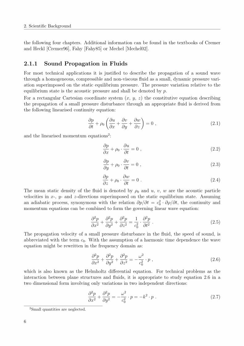
2.1.1 Sound Propagation in Fluids
For most technical applications it is justified to describe the propagation of a sound wavethrough a homogeneous, compressible and non-viscous fluid as a small, dynamic pressure vari-ation superimposed on the static equilibrium pressure. The pressure variation relative to theequilibrium state is the acoustic pressure and shall be denoted by p.
For a rectangular Cartesian coordinate system (x, y, z) the constitutive equation describingthe propagation of a small pressure disturbance through an appropriate fluid is derived fromthe following linearised continuity equation:
∂p
∂t+ ρ0
(∂u
∂x+∂v
∂y+∂w
∂z
)= 0 , (2.1)
and the linearised momentum equations2:
∂p
∂x+ ρ0 ·
∂u
∂t= 0 , (2.2)
∂p
∂y+ ρ0 ·
∂v
∂t= 0 , (2.3)
∂p
∂z+ ρ0 ·
∂w
∂t= 0 . (2.4)
The mean static density of the fluid is denoted by ρ0 and u, v, w are the acoustic particlevelocities in x-, y- and z-directions superimposed on the static equilibrium state. Assumingan adiabatic process, synonymous with the relation ∂p/∂t = c20 · ∂ρ/∂t, the continuity andmomentum equations can be combined to form the governing linear wave equation:
∂2p
∂x2+∂2p
∂y2+∂2p
∂z2=
1
c20· ∂
2p
∂t2. (2.5)
The propagation velocity of a small pressure disturbance in the fluid, the speed of sound, isabbreviated with the term c0. With the assumption of a harmonic time dependence the waveequation might be rewritten in the frequency domain as:
∂2p
∂x2+∂2p
∂y2+∂2p
∂z2= −ω
2
c20· p , (2.6)
which is also known as the Helmholtz differential equation. For technical problems as theinteraction between plane structures and fluids, it is appropriate to study equation 2.6 in atwo dimensional form involving only variations in two independent directions:
∂2p
∂x2+∂2p
∂y2= −ω
2
c20· p = −k2 · p . (2.7)
2Small quantities are neglected.
6

2.1 Structural Sound Transmission
A general solution for the plane wave propagation is given by:
p(x, y, t) = p · e−jkxx · e−jkyy · ejωt , (2.8)
in which p is a complex pressure magnitude and k the wavenumber defined as k = ω/c0. Thewavenumber represents the magnitude of a vector indicating the direction of propagation andalso describes the phase change per unit increase of distance. Inserting the above expression inequation 2.7 yields in the following relation for the wavenumber k and its x- and y-components:
k2 = k2x + k2
y , (2.9)
which must be satisfied for kx and ky at any given frequency to be a solution for the waveequation. The direction of the wave is given by the angle φ between the vector k and thex-axis. φ is determined by the relations:
sinφ = ky/k and cosφ = kx/k . (2.10)
Furthermore, the momentum equations 2.2 to 2.4 relate the spatial pressure gradient in agiven direction to the particle acceleration in that direction. Assuming a harmonic time de-pendence, the acceleration can be expressed by the velocity and the momentum equationbecomes ∂p/∂n = −jω ·ρ0 · vn, where n denotes an arbitrary direction vector. The momentumrelation is also appropriate to describe the boundary condition for the sound radiation andfluid loading on a vibrating fluid-structure interface. Thus, the normal velocity of a structuresurface determines the normal pressure gradient of the fluid and vice versa. Assuming a sur-face lying in the y,z-plane and using the plane wave field from equation 2.8, the momentumequation (∂p/∂x)x=0 = −jω · ρ0 · ux=0 becomes:
kx · px=0 = ω · ρ0 · ux=0 = k · ρ0 · c0 · ux=0 = k · Z0 · ux=0 , (2.11)
since Z0 is the acoustic impedance of a free plane wave given by the ratio of its acoustic pressureand particle velocity, Z0 = p/u = ρ0 · c0.
2.1.2 Bending Waves in Thin Plates
For an infinite and uniform thin plate of thickness h, subjected to a transversal excitation perunit area p, the one dimensional bending equation is:
D · (1 + jη) · ∂4w
∂x4+m · ∂
2w
∂t2= p · ej(ωt−kx) , (2.12)
with the bending stiffness D defined as D = E · h3/12/(1 − ν2) and the mass per unit aream = ρ · h. Damping is represented by the introduction of a complex Young’s modulus3. Ageneral solution to equation 2.12 can be expressed as:
w(x, t) = w · ej(ωt−kx) , (2.13)
3E′ = E · (1 + jη), with η being defined as loss factor.
7

2. Scientific Background
where w is the complex amplitude of the transversal displacement w and k the wavenumberspecified by the frequency ω and the phase speed cb in the plate, k = ω/cb. Introducing theabove expression for the flexural wave in equation 2.12 yields:
(D · (1 + jη) · k4 −m · ω2) · w = p . (2.14)
The ratio of the complex pressure magnitude to the complex velocity magnitude defines thestructural wave impedance of the plate and takes the form:
Zwp =p
jω · w = −j · (D · k4 −m · ω2)/ω +D · k4 · η/ω . (2.15)
The solution of the homogeneous, undamped bending equation 2.14 yields the free-plate bend-ing wavenumber kb = (ω2 ·m/D)1/4 and the phase speed cb = (ω2 ·D/m)1/4. For an excitationwith k = kb an infinite small force per unit area causes an infinite large displacement and thewave impedance of the plate Zwp becomes zero.
2.1.3 Sound Transmission through Infinite Single Wall Partitions
The sound transmission through an infinite partition separating two fluid domains can beregarded as a boundary value problem on the partition surface. Considering the system repre-sented in Figure 2.1 the partition in the y,z-plane separates two acoustic domains characterizedby impedances Z1 = ρ1 · c1 and Z2 = ρ2 · c2. An acoustic plane wave Pi is incident upon thepartition from the left side with an angle of φ1.
x
y
c >c ,2 1 2r
Fluid 2
Pr
Fluid 1
c ,1 1r
Pt
Pi
f1
f2
v
Figure 2.1: Transmission of oblique sound waves through an infinite single wall partition
The incident, reflected and transmitted pressure sound field may be written as4:
pi(x, y) = Pi · e−jk1,xx · e−jk1,yy , (2.16)
4The term ejωt is omitted in the following.
8

2.1 Structural Sound Transmission
pr(x, y) = Pr · ejk1,xx · e−jk1,yy = r · Pi · ejk1,xx · e−jk1,yy , (2.17)
pt(x, y) = Pt · e−jk2,xx · e−jk2,yy . (2.18)
In equation 2.17 the abbreviation r denotes the reflection coefficient defined as the ratio betweenthe complex magnitude of the reflected wave to the complex magnitude of the incident wave.Furthermore, equation 2.9 and 2.10 must be satisfied for the wavenumber and its x- and y-components in both fluid domains. In addition, the trace wavenumber ki,y is the same on bothsides and in the partition, hence k1,y = k2,y = ky or:
sinφ2/ sinφ1 = c2/c1 . (2.19)
The transversal plate velocity is formulated as:
v(y) = V · e−jkyy . (2.20)
The momentum equation 2.2 at x = 0 yields the boundary conditions for the particle velocityon the surface of the partition:
v(0, y) = (Pi − Pr) · cosφ1 · e−jkyy/Z1 = Pi · (1 − r) · cosφ1 · e−jkyy/Z1 , (2.21)
v(0, y) = Pt · cosφ2 · e−jkyy/Z2 . (2.22)
The effective load on the partition is equal to the pressure difference on both sides and fromthe bending wave equation 2.14 follows the relation:
Zwp · V · e−jkyy = (Pi · (1 + r) − Pt) · e−jkyy . (2.23)
Eliminating the reflection coefficient r and velocity magnitude V the complex pressure ratioPt/Pi is derived from equation 2.21 to 2.23:
Pt
Pi
=2 · Z2 · cosφ1
Z2 · cosφ1 + Zwp · cosφ1 · cosφ2 + Z1 · cosφ2
. (2.24)
The transmission coefficient τ relates the transmitted to the incident sound power:
τ =
∣∣∣Pt
∣∣∣2
· cosφ2/2ρ2c2∣∣∣Pi
∣∣∣2
· cosφ1/2ρ1c1
, (2.25)
and the sound transmission index R is given by5:
R = 10 · log(τ−1) [dB] . (2.26)
If the fluid on both sides of the partition is the same, equation 2.25 is reduced to:
5Also denoted as transmission loss TL in literature.
9

2. Scientific Background
τ =2 · Z0
2 · Z0 + Zwp · cosφ, (2.27)
since φ1 = φ2 = φ and Z1 = Z2 = Z0. Replacing the term Zwp with the expression 2.15 for thewave impedance of the thin plate results in:
τ =(2 · Z0/ cosφ)2
(2 · Z0/ cosφ+ (D/ω) · η · k4 · sin4 φ
)2+
(ω ·m− (D/ω) · k4 · sin4 φ
)2 , (2.28)
which can be further simplified by introducing the expression for the free flexural wavenumberkb:
τ =(2 · Z0/ωm cosφ)2
(2 · Z0/ωm cosφ+ (k/kb)4 · η · sin4 φ
)2+
(1 − (k/kb)4 · sin4 φ
)2 . (2.29)
If the trace wavenumber ky is equal to the wavenumber of the free bending wave in the plate,ky = k · sinφ = kb = (ω2 ·m/D)1/4, the reactive term of the wave impedance in equation 2.15disappears and the transmission coefficient τ exhibits a local maximum. Therefore, with theassumption of an undamped structure, the incident sound wave will be totally transmittedinto the second fluid domain and τ will be equal to one. This characteristic is referred to ascoincidence and has a similar impact on the spatial periodicity as the resonance phenomenonfor the temporal periodicity. For each angle of incidence the frequency connected with thecoincidence phenomenon is given by the following relation:
ωco = (c0/sinφ)2 · (m/D)1/2 . (2.30)
Since the term sinφ is always less than or equal to unity, the coincidence frequency ωco cannotfall below a lower limit, which is designated as critical frequency or lowest coincidence frequencyωc:
ωc = c20 · (m/D)1/2 . (2.31)
The above equation shows that the critical frequency is proportional to term (m/D)1/2. Thus,a stiff partition will have a lower critical frequency than a less stiff partition of similar weight.
It is now appropriate to analyse the sound transmission coefficient in dependence of the fre-quency ratio ω/ωc = (k/kb)
2. For ω ≪ ωc the stiffness and damping terms, (D/ω) · k4 · sin4 φand (D/ω) · η · k4 · sin4 φ respectively, can be neglected in comparison to the inertia term ω ·mand the transmission coefficient τ is approximated by the relation:
τ(φ) ≈(1 + (ω ·m · cosφ/2Z0)
2)−1. (2.32)
Assuming that ω ·m · cosφ≫ 2 · Z0, the sound reduction index may be written as:
R(φ) = 20 · log (ω ·m · cosφ/2Z0) [dB] . (2.33)
10
2.1 Structural Sound Transmission
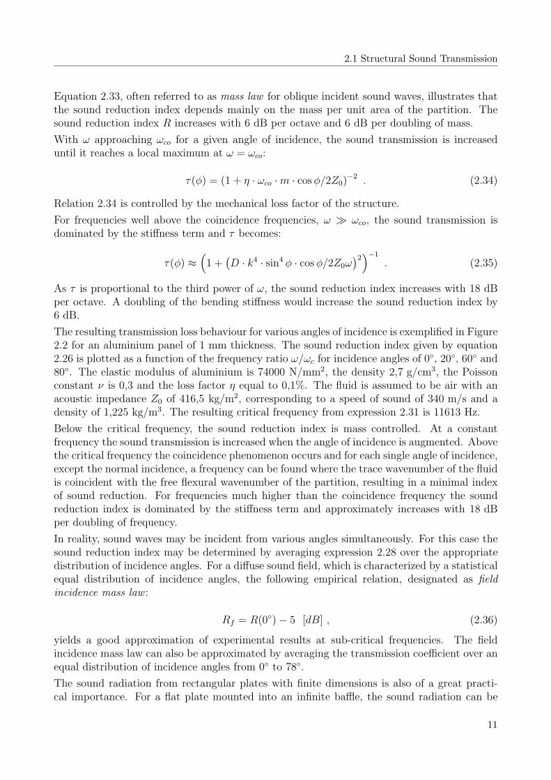
Equation 2.33, often referred to as mass law for oblique incident sound waves, illustrates thatthe sound reduction index depends mainly on the mass per unit area of the partition. Thesound reduction index R increases with 6 dB per octave and 6 dB per doubling of mass.
With ω approaching ωco for a given angle of incidence, the sound transmission is increaseduntil it reaches a local maximum at ω = ωco:
τ(φ) = (1 + η · ωco ·m · cosφ/2Z0)−2 . (2.34)
Relation 2.34 is controlled by the mechanical loss factor of the structure.
For frequencies well above the coincidence frequencies, ω ≫ ωco, the sound transmission isdominated by the stiffness term and τ becomes:
τ(φ) ≈(1 +
(D · k4 · sin4 φ · cosφ/2Z0ω
)2)−1
. (2.35)
As τ is proportional to the third power of ω, the sound reduction index increases with 18 dBper octave. A doubling of the bending stiffness would increase the sound reduction index by6 dB.
The resulting transmission loss behaviour for various angles of incidence is exemplified in Figure2.2 for an aluminium panel of 1 mm thickness. The sound reduction index given by equation2.26 is plotted as a function of the frequency ratio ω/ωc for incidence angles of 0, 20, 60 and80. The elastic modulus of aluminium is 74000 N/mm2, the density 2,7 g/cm3, the Poissonconstant ν is 0,3 and the loss factor η equal to 0,1%. The fluid is assumed to be air with anacoustic impedance Z0 of 416,5 kg/m2, corresponding to a speed of sound of 340 m/s and adensity of 1,225 kg/m3. The resulting critical frequency from expression 2.31 is 11613 Hz.
Below the critical frequency, the sound reduction index is mass controlled. At a constantfrequency the sound transmission is increased when the angle of incidence is augmented. Abovethe critical frequency the coincidence phenomenon occurs and for each single angle of incidence,except the normal incidence, a frequency can be found where the trace wavenumber of the fluidis coincident with the free flexural wavenumber of the partition, resulting in a minimal indexof sound reduction. For frequencies much higher than the coincidence frequency the soundreduction index is dominated by the stiffness term and approximately increases with 18 dBper doubling of frequency.
In reality, sound waves may be incident from various angles simultaneously. For this case thesound reduction index may be determined by averaging expression 2.28 over the appropriatedistribution of incidence angles. For a diffuse sound field, which is characterized by a statisticalequal distribution of incidence angles, the following empirical relation, designated as fieldincidence mass law :
Rf = R(0) − 5 [dB] , (2.36)
yields a good approximation of experimental results at sub-critical frequencies. The fieldincidence mass law can also be approximated by averaging the transmission coefficient over anequal distribution of incidence angles from 0 to 78.
The sound radiation from rectangular plates with finite dimensions is also of a great practi-cal importance. For a flat plate mounted into an infinite baffle, the sound radiation can be
11

2. Scientific Background
10−2
10−1
100
0
10
20
30
40
50
60
70Transmission Loss
Frequency / Critical Frequency [−]
TL
[dB
]Normal Incidence20° Incidence40° Incidence60° Incidence80° Incidence
Figure 2.2: Transmission loss of an infinite single wall partition for various angles of incidence
calculated with the Rayleigh integral approach [Fahy85]. This requires the knowledge of thecomplex velocity distribution on the plate, which is composed of many superimposed modalcontributions. Consequently, at low frequencies6, the sound radiation is strongly governed bysingle vibrational eigenmodes. Each mode is associated with a certain radiation efficiency,which depends on the structural properties and boundary effects [Berry90, Wallace72]. Ingeneral odd modes are efficient radiators, resulting in a low transmission loss and even modesare less efficient radiators. Thus, at low frequencies, the TL behaviour of a finite partition ischaracterised by the succession of resonance and anti-resonance peaks. At high frequencies,where the structural response is governed by the superposition of multiple eigenmodes, thesound radiation from a finite partition is similar to the one from an infinite plate.
2.1.4 Sound Transmission through Infinite Double Wall Partitions
As it was shown in the previous chapter, for sub-critical frequencies, which in most cases covera large part of the audible frequency range, the sound transmission of a single wall structuredepends mainly on the mass per unit area of the employed partition. However, in practiceit is often mandatory to have lightweight structures that provide a high sound reduction atthe same time, two requirements being totally antipodal. A typical application would be anaircraft fuselage.
Nevertheless, it is possible to meet such requirements by employing partitions consisting of two
6The acoustical wavelength is large in comparison to a characteristic dimension of the plate.
12

2.1 Structural Sound Transmission
or more walls being separated by fluid cavities. In a simple model for this configuration, theair in the cavity might be primarily seen as mechanical stiffness acting between the individualmasses of the adjacent partitions. Depending on the excitation frequency, the cavity fluid leadsto an effective decoupling of the structural behaviour of adjoining leaves and thus to a hightransmission loss, but at resonance frequencies a strong coupling might occur, resulting in asound reduction index that might be lower than the one given for a single leaf of the sametotal mass.
To demonstrate the behaviour of such systems a generic double wall partition, as depictedin Figure 2.3, is analysed theoretically. The setup consists of two infinite and homogeneouspartitions separated by a distance d. It is assumed that the fluid on both sides as well as inthe cavity has the same properties. The problem of sound transmission through the doublewall system is solved in analogous manner as for the single wall partition.
Pb Pa
v2
x
y
Fluid
c ,0 r0
Pt
f
d
Pr
f
Pi
v1
Figure 2.3: Transmission of oblique sound waves through an infinite double wall partition
The formulations for the incident, reflected and transmitted sound fields can be adopted fromequation 2.16 to 2.18. In the cavity, the pressure results from the wave transmitted by the firstpartition as well as from a wave reflected by the second partition:
pa(x, y) = Pa · e−jkxx · e−jkyy , (2.37)
pb(x, y) = Pb · ejkxx · e−jkyy . (2.38)
With the plate velocities given by the following relations:
v1(y) = V1 · e−jkyy , (2.39)
v2(y) = V2 · e−jkyy , (2.40)
the boundary conditions obtained from the momentum equations applied to the first partitionfollow as:
13

2. Scientific Background
v1(0, y) = Pi · (1 − r) · cosφ · e−jkyy/Z0 , (2.41)
v1(0, y) = (Pa − Pb) · cosφ · e−jkyy/Z0 , (2.42)
and for the second partition as:
v2(d, y) = (Pa · e−jkxd − Pb · ejkxd) · cosφ · e−jkyy/Z0 , (2.43)
v2(d, y) = Pt · cosφ · e−jkxd · e−jkyy/Z0 , (2.44)
where kx = k · cosφ and ky = k · sinφ as defined in equation 2.10. The bending wave equationyields a further expression for each partition:
Zwp,1 · V1 · e−jkyy =(Pi · (1 + r) − (Pa + Pb)
)· e−jkyy , (2.45)
Zwp,2 · V2 · e−jkyy =(Pa · e−jkxd + Pb · ejkxd − Pt · e−jkxd
)· e−jkyy . (2.46)
Resolving equations 2.16 to 2.18 and 2.37 to 2.46 for the pressure ratio of the transmitted tothe incident sound field results in:
Pt
Pi
=−2 · j · Z2
0 · sin (kd · cosφ)/ cos2 φ
Z1 · Z2 · sin2 (kd · cosφ) + Z20/ cos2 φ
, (2.47)
with Zi used as an abbreviation for the term:
Zi = Zwp,i + Z0 ·(1 − j · tan−1 (kd · cosφ)
)/ cosφ . (2.48)
In the low-frequency range, when the acoustic wavelength is much greater than the partitionseparation distance, kd · cosφ≪ 1, equation 2.47 is simplified to:
Pt
Pi
≈ −2 · j · Z20/(kd · cosφ)
Z1 · Z2 + Z20/(kd · cosφ)2
, (2.49)
with Zi = Zwp,i · cosφ + Z0 − j · Z0/(kd · cosφ). The term Zi represents the combination of astructural wave impedance Zwp,i (defined by a stiffness, inertia and damping term as given inequation 2.15) with an acoustic damping term Z0 and an acoustic stiffness term Z0/(kd ·cosφ).The ratio of mechanical to acoustic stiffness can be expressed as:
δ =D · (k · sinφ)4/ω
Z0/(kd · cosφ), (2.50)
and is usually far less than unity for typical lightweight structures and air as fluid. Thus, theacoustical and mechanical damping as well as the mechanical stiffness can be neglected andthe pressure transmission ratio Pt/Pi is reduced to:
14

2.1 Structural Sound Transmission
Pt
Pi
≈ −2 · j · Z20/(kd · cosφ)
ω · Z0 · (m1 +m2)/kd− ω2 ·m1 ·m2 · cos2φ. (2.51)
The above expression for the pressure ratio becomes infinite, when the denominator in equation2.51 equals zero. This condition is fulfilled for the frequency ωr:
ωr =
(Z0 · c · (m1 +m2)
d ·m1 ·m2 · cos2φ
)1/2
= ω0 · cos−1φ . (2.52)
The frequency ωr is designated as the mass-air-mass resonance with ω0 being the frequencyof the fundamental mass-air-mass resonance for normal incidence. ωr increases for decreasingvalues of partition separation distance d and is minimal when m1 = m2 for a total given massmt = m1 +m2.
For frequencies well below the mass-air-mass resonance the following conditions apply: ω ≪ ωr
and ω2 ·m1 ·m2 · cos2φ≪ (m1 +m2) ·Z0 · c/d. Therefore, the term ω2 ·m1 ·m2 · cos2φ may beneglected in equation 2.51 and the pressure ratio becomes:
Pt
Pi
≈ −2 · j · Z0
ω · (m1 +m2) · cosφ, (2.53)
or equally expressed by the sound reduction index R:
R(φ) ≈ R(φ,mt) [dB] , (2.54)
which is similar to the behaviour of a single-wall partition with the mass mt = m1 +m2.
If the frequency is approaching the mass-air-mass resonance ωr, the mechanical damping ofthe partitions may not be neglected anymore. At the frequency ω = ωr the pressure ratio is:
Pt
Pi
=−2 · j · Z0/cosφ
ω · (η1 ·m2 + η2 ·m1) + Z0 · (m21 +m2
2)/m1m2cosφ. (2.55)
In the frequency range above the resonance, ω2 · m1 · m2 · cos2φ > (m1 + m2) · Z0 · c/d, thepressure ratio is inertia dominated and can be approximated as:
Pt
Pi
≈ 2 · j · Z0 · ω20
ω3 · cos3 φ · (m1 +m2), (2.56)
with the corresponding sound reduction index given by:
R(φ) ≈ R(φ,mt) + 40 · log((ω/ω0) · cosφ) [dB] . (2.57)
As the pressure ratio is proportional to the third power of the frequency, a doubling of frequencyis increasing the sound reduction index by 18 dB.
For the high-frequency range the variation of sound transmission with the frequency has tobe analysed by using the exact solution of equation 2.47. In general, it can be said that thesound transmission behaviour is characterized by a succession of acoustic anti-resonances andresonances occurring in the cavity. The anti-resonance and resonance condition are kd ·cosφ =
15

2. Scientific Background
(2n − 1) · π/2 and kd · cosφ = n · π respectively, with n being any integer greater than zero.Neglecting the stiffness and damping terms in equation 2.47, the estimation for the pressuretransmission ratio at anti-resonance frequencies becomes:
Pt
Pi
≈ 2 · j · Z20
ω2 ·m1 ·m2 · cos2 φ. (2.58)
Hence, the sound reduction index takes the approximate form of:
R(φ) ≈ R(φ,m1) +R(φ,m2) + 6 [dB] , (2.59)
and increases with a rate of 12 dB per octave. Equation 2.59 represents the upper limit forthe transmission loss behaviour in the high-frequency range.
At cavity resonance frequencies it is derived from equation 2.42 and 2.43 that the displacementof both partitions must be the same and the sound reduction index follows as:
Pt
Pi
=2 · Z0/ cosφ
Z1 + Z2 + 2 · Z0/ cosφ. (2.60)
With the assumption that the denominator in the above equation is dominated by the inertiaterm, the sound reduction index corresponds to the one given by a single leaf with the massmt = m1 +m2:
R(φ) ≈ R(φ,mt) [dB] . (2.61)
The general variation of the sound reduction index with the frequency is shown in the followingtwo figures considering as example a double wall partition made of 1 mm thick aluminiumsheets. The same material properties as for the previous example are used. The separationdistance of the leaves is 50 mm. Figure 2.4 shows the influence of various incidence angles(normal incidence, 20, 40 and 60) for frequencies ranging from 50 Hz to 20 kHz.
Below the fundamental mass-air-mass resonance, which occurs here at 231 Hz, the behaviouris that of a single leaf with mt = m1+m2. At the resonance frequencies the sound transmissionbehaviour is very much similar to the coincidence phenomenon. Above the fundamental mass-air-mass resonance and each cavity resonance for normal incidence (in the example occurringat multiples of 3,4 kHz) exists a frequency and an angle of incidence where a strong couplingbetween the cavity and the partition leaves occurs, resulting in a local TL minimum. Thus, fora diffuse field excitation, the sound transmission is controlled by resonant effects. Coincidenceeffects are also observed as for a single leave partition. They are particularly strong for systemsconsisting of identical panels. In the given example this is evident for the case with 60
incidence, where the coincidence occurs at a frequency of 15484 Hz.
Illustrated in Figure 2.5 is the dependency of the sound reduction index on the mass ratio λ =m1/m2. Using the same configuration as in the previous example and a normal incident soundfield, the overall weight per unit area of the double wall partition is kept constant (5,4 kg/m2),while varying the thickness ratio of the partitions. For identical partitions with λ = 1 thevalue of the sound reduction index at the mass-air-mass resonance ω0 is minimized, whereasin the frequency range where cavity resonances occur, the upper limit of sound reduction ismaximised by making m1 = m2. For values of m1/m2 or m2/m1 ≫ 1 the transmission loss
16

2.1 Structural Sound Transmission
102
103
104
−20
0
20
40
60
80
100
120Transmission Loss
Frequency [Hz]
TL
[dB
]Normal Incidence20° Incidence40° Incidence60° Incidence
Figure 2.4: Transmission loss of an infinite double wall partition for various angles ofincidence
102
103
104
0
20
40
60
80
100
120Transmission Loss
Frequency [Hz]
TL
[dB
]
Mass Ratio λ = 1Mass Ratio λ = 10Mass Ratio λ = 30
Figure 2.5: Transmission loss of an infinite double wall partition for various mass ratios
17

2. Scientific Background
is increased at ω0 but at the same time the maxima at cavity anti-resonances frequencies arelowered.
In addition, it should be noted that in practice layers of porous sound-absorbing materials aredisposed into cavities to minimise resonant sound transmission. Depending on the materialtype and the frequency range the resonant coupling of the cavity to the partition leaves can bereduced to a large extent by the additional acoustic dissipation [Beranek49, Fahy85, Ingard94].
2.2 Aircraft Interior Noise
Aircraft interior noise represents an important point in the design process and operation ofaircraft as intense interior noise levels may result in a feeling of discomfort for the passengers,increase the crew workload and fatigue, interfere with the internal crew communication anddisturb the proper functioning of electronic equipment. Noise control measures are thereforerequired to assure an acceptable interior noise environment. However, they usually also resultin penalties as increased structural weight or reduced cabin volume, which makes it difficultto determine the best compromise in efficient noise reduction and inevitable penalties.
2.2.1 Noise Sources
Main sources of interior noise are various contributions from the propulsion system such asthe jet mixing and turbomachinery noise, the turbulent aerodynamic boundary flow aroundthe vehicle and different aircraft systems such as hydraulics or air conditioning for instance.External noise sources as the engines or the turbulent flow around the fuselage impinge directlythe fuselage skin and are propagated as airborne and structure-borne noise into the interior.Mechanical sources such as an unbalanced engine or structural, flow-induced vibrations aretransmitted as structure-borne noise along the fuselage and radiated into the cabin. Eachsource has its own characteristics and local contributions are also dependant on the flightconditions. A short description of the main sources for modern subsonic civil aircraft fittedwith high bypass-ratio turbofan jet engines is given in the following sections. A comprehensivesummary can be found in the textbooks of [Braunling04, Groeneweg95, Lilley95, Mixson95].
Jet Mixing Noise
A significant type of noise for any jet aircraft is the jet mixing noise. It is caused by theturbulent mixing process of the engine’s exhaust stream with the ambient air. As indicated byLighthill’s acoustic analogy [Lilley95], the jet mixing noise is a strong function of jet exhaustvelocity, namely depending on the sixth to eighth power of velocity. The development ofengines with greater propulsive and fuel efficiency during the last decades led to increasedbypass ratios, hence reducing the average exhaust velocity and jet noise levels. Even so, jetnoise remains a main source of aircraft noise and its suppression is still subject of intensivestudies.
The mixing process of the hot jet core and cold bypass exhausts with the atmosphere producesa broadband, haystack-shaped sound frequency spectrum. The shape of the spectrum reflectsthe fact that the turbulence structures that comprise the mixing process vary considerably,
18

2.2 Aircraft Interior Noise
increasing in size progressively downstream of the exhaust nozzle and decaying in intensity asthe average exhaust velocity decreases and the mixing becomes complete. Due to convectionand refraction effects the maximum sound intensity is radiated at oblique angles to the down-stream direction of the jet. The sound perturbations impinging the fuselage structure may beconsidered with a spatially coherent excitation having a certain directivity pattern for a givenflight condition. In comparison to a subsonic turbulent boundary layer noise excitation, jetnoise is more efficient at exciting structural vibrations at lower frequencies and especially inthe aircraft aft section interior noise may be dominated by jet noise components.
Turbomachinery Noise
In modern, high bypass ratio engines the major turbomachinery noise contribution is due tothe fan. It contains three components: pure tones at the blade-passing frequency (BPF) andits harmonics, broadband noise and buzz-saw noise7. Turbomachinery noise represents theprinciple source of tonal noise in the cabin. Secondary sources such as the compressor andturbine stage typically produce only little contribution to the overall radiated turbomachinerynoise.
The dominant sources of fan tone noise at the blade-passing frequency and its harmonics areusually excited by a rotor-stator interaction, where coherent parts of fan wakes interact withdownstream stators and struts. Its fundamental frequency is given by the relation fBPF = n·B,where B is the number of fan blades and n the rotational speed of the fan shaft. The polardirectivity pattern for discrete tones can be highly irregular depending on the actual sourcemechanism and frequency. Broadband noise is mainly due to turbulent flow inhomogeneities.The turbulence may result from the inflow in the engine, the inlet boundary layer, the bladewakes, or the blade tip vortices interacting with each other. To suppress fan and other inter-nally generated turbomachinery noise the inlet and fan exhaust ducts of modern commercialtransport aircraft are equipped with acoustic liners designed to absorb the sound generated bythe various sources.
The third major component of turbomachinery noise is due to the fact that modern aero-engines use transonic fans. The fans are operated with supersonic relative speeds at the tipsresulting in a further source known as buzz-saw noise [McAlpine01]. The flow approachingeach blade passes through the shock waves associated with the adjacent blades and, as no twoblades can be made absolutely uniform, the resultant shock pattern is unique to each blade andvaries around the rotor due to the manufacturing tolerance. Hence, tonal sound is generatedat a series of frequencies, which are multiples of the rotation speed. The dominant acousticenergy is concentrated at frequencies below and at the BPF. With higher local Mach numbersat the blade tips, low order harmonics tend to become the predominant source. The actualsound radiation is also strongly dependant on highly non-linear duct propagation phenomenaas the rotating shock-wave pattern is spread in upstream direction through the inlet duct.Under certain conditions, mainly during take-off and climb, the buzz-saw noise mechanism candominate the forward arc of the polar directivity radiation pattern as the main acoustic energyis radiated at angles of around 45 with respect to engine centreline [Lewy00]. Thus, buzz-sawnoise can be clearly audible for the passengers, especially in the forward cabin.
7Also described as multiple pure tones or combination tones in literature.
19
2. Scientific Background
Turbulent Boundary Layer Noise (TBL)
In cruise condition the turbulent boundary layer pressure field acting on the fuselage skin isin general the dominant source of noise in the forward and mid-cabin of high subsonic andsupersonic commercial aircraft. For interior noise it represents the only non-engine relatedperturbation source. The structure of the turbulent pressure field depends on the Reynoldand Mach numbers, the surface roughness, the pressure gradient and the velocity field outsidethe boundary layer. TBL noise is highly statistical in both space and time. Thus, dependingon the flight condition and the location along the fuselage axis, its spectral density containsbroadband components from below 100 Hz up to 2 kHz. To predict the sound transmissionthrough a structure excited by a TBL pressure field one needs to know the local propertiesof the turbulent boundary layer, which is still the subject of intense research. A first semi-empirical description of the TBL field was derived with the Corcos formulation, which is basedon the cross spectral densities of the pressure fluctuations [Corcos63]. For more approximatepredictions less accurate empirical relations might be used [Ungar77].
Structure-Borne Noise
Structural vibrations, acting on distant regions of the airframe and being transmitted as vibra-tion into the fuselage and the cabin, represent an additional source of interior noise. In contrastto the aforementioned components, which can be resumed under the term airborne noise, theyare referred to as structure-borne noise. Known causes are, for instance, engine unbalanceforces, especially on aircraft with aft engine-mount configurations and unsteady aerodynamicflows such as the wake of a propeller striking the wing or the tail. Further known sourcesare hydraulic pumps, air conditioning systems and other rotating equipment. Structure-bornenoise is mainly associated with discrete perturbation frequencies.
2.2.2 Sound Transmission
The various airborne and structure-borne primary excitations impinging the fuselage are fil-tered by the structural response and then radiated into the cabin. Figure 2.6 shows an exem-plary interior noise spectrum up to 600 Hz for a typical single aisle aircraft. It was measured inthe forward cabin for two different flight conditions, climb and cruise. During the take off andclimb phase tonal noise components due to a strong buzz-saw noise excitation are clearly audi-ble in the broadband noise spectrum. The fundamental frequency is 79 Hz and corresponds tothe shaft speed of the fan. In cruise condition all but one tonal component disappear, but theoverall broadband noise caused by the jet and TBL noise primary perturbations is increased forfrequencies above 200 Hz. The fundamental buzz-saw noise tone does not disappear, indicatinga possible structure-borne sound transmission in this particular case and is reduced to 62 Hzas the engine thrust and speed is reduced for cruise. By cancelling the buzz-saw noise tonesand reducing the broadband noise level the aircraft interior noise and the passenger comfortcould be largely improved.
For airborne noise components, which are the major contributors to interior noise, the struc-tural response characteristic may be described with the transmission loss behaviour of theaircraft sidewall [May85]. In passenger aircraft the sidewall represents a double wall multi-element system consisting of the fuselage structure, fibreglass blankets, impervious septa, an
20

2.2 Aircraft Interior Noise
0 100 200 300 400 500 600 7000
5
10
15
20
25
30
35
40
45
Frequency [Hz]
Rel
ativ
e S
ound
Pre
ssur
e [d
B]
Narrowband Pressure Magnitude Spectrum
Climb after Take−OffCruise
Figure 2.6: Single aisle interior noise spectrum
interior decorative trim panel and multi-pane windows. The fibreglass blankets are used forinterior noise control issues and also provide the required heat insulation.
In contrast to the analytical mass law presented in Chapter 2.1.4 the sound transmissionbehaviour is more complex as a conventional aircraft structure consists of the fuselage skin,which is supported by longitudinal and circumferential stiffeners (stringers and frames). De-tailed analytical models and measurements have shown that at low frequencies the skin andstiffeners vibrate in phase with the same magnitude. Thus, the mechanical properties can besmeared over a certain sidewall area and an equivalent orthotropic structural behaviour canbe assumed. At high frequencies the structural wavelength becomes much shorter than thestiffener spacing and the stiffener motion can be neglected in comparison to the out-of-planedisplacement of the skin. Hence, acoustic perturbations are mainly transmitted by vibrating,local skin patches. The validity of the simplifications is dependent on the actual mechanicalproperties of the considered fuselage structure. In the mid-frequency range in-between thosebehaviours both the skin and stiffener motions are strongly coupled and must be consideredin detail for an analysis of sound transmission.
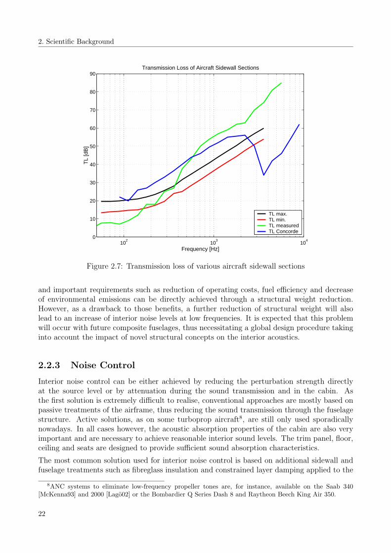
Some typical transmission loss curves for different aircraft sidewall structures available fromliterature [Tran95, Wilby73] are shown in Figure 2.7. Their common characteristic is the ratherpoor reduction of sound transmission in the low-frequency range up to 400 or 500 Hz. Aspassive treatments like fibreglass wool are not providing efficient absorption capabilities in thisparticular range of frequency [Thomas02], the transmission loss is mainly governed by the masslaw with the structural mass of the aircraft sidewall being the main parameter. On the otherhand, structural mass represents also a global variable in the overall aircraft design process
21
2. Scientific Background
102
103
104
0
10
20
30
40
50
60
70
80
90Transmission Loss of Aircraft Sidewall Sections
Frequency [Hz]
TL
[dB
]
TL max.TL min.TL measuredTL Concorde
Figure 2.7: Transmission loss of various aircraft sidewall sections
and important requirements such as reduction of operating costs, fuel efficiency and decreaseof environmental emissions can be directly achieved through a structural weight reduction.However, as a drawback to those benefits, a further reduction of structural weight will alsolead to an increase of interior noise levels at low frequencies. It is expected that this problemwill occur with future composite fuselages, thus necessitating a global design procedure takinginto account the impact of novel structural concepts on the interior acoustics.
2.2.3 Noise Control
Interior noise control can be either achieved by reducing the perturbation strength directlyat the source level or by attenuation during the sound transmission and in the cabin. Asthe first solution is extremely difficult to realise, conventional approaches are mostly based onpassive treatments of the airframe, thus reducing the sound transmission through the fuselagestructure. Active solutions, as on some turboprop aircraft8, are still only used sporadicallynowadays. In all cases however, the acoustic absorption properties of the cabin are also veryimportant and are necessary to achieve reasonable interior sound levels. The trim panel, floor,ceiling and seats are designed to provide sufficient sound absorption characteristics.
The most common solution used for interior noise control is based on additional sidewall andfuselage treatments such as fibreglass insulation and constrained layer damping applied to the
8ANC systems to eliminate low-frequency propeller tones are, for instance, available on the Saab 340[McKenna93] and 2000 [Lago02] or the Bombardier Q Series Dash 8 and Raytheon Beech King Air 350.
22
2.3 Piezoelectricity
fuselage skin [Mixson95] or the trim. The additional treatments have to satisfy numerous con-straints such as thermal insulation, fireproofing, moisture-resistance and, above all, must haveminimum weight and volume [May85]. Fibreglass blankets meet all the above requirementsand are available in various densities from about 6 to 24 kg/m3. Fibreglass is most efficientagainst broadband noise at frequencies greater than 500 Hz, where it provides a good additionalnoise reduction compared to the untreated double wall section. An improvement of the noisereduction at lower frequencies requires additional weight and can be achieved by introducingan impervious septa, such as lead-impregnated vinyl, between the layers of porous material.
In addition to the use of sidewall treatments, the noise transmission and acoustic radiationcharacteristics of fuselage structures can be modified by the addition of mass, damping orstiffness [Mixson95]. Damping is the most common method. The existing damping in fuselageskins is usually very small with values of about 1% and can be raised up to 5% by addingdamping material (i.e. aluminium-backed tape) to the interior side of the skin, between thering frames and stringers. This method is particularly adapted for resonant responses, forexample the hydrodynamic coincidence between the turbulent boundary layer and local skinmodes. The additional damping and mass change the dynamical behaviour of the structure,thus attenuating resonant excitations. However, appropriate materials have to be used as thefuselage skin temperature can decrease below -50C during cruise. Measurements on large,modern jet aircraft have shown that interior sound pressure levels could thus be reduced by 3to 8 dB above 800 Hz. Damping material can also be applied to other structural parts if theirsound transmission and radiation behaviour is dominated by resonant components.
Further passive solutions are also utilised in aircraft applications. Dynamic vibration absorberswith tuned resonance frequencies are mainly used to reduce tonal noise components duringcruise. Typical applications are the reduction of propeller noise in turboprop aircraft, whereabsorbers tuned to low harmonics of the propeller noise are installed on the ring frames andtrim panels [Wright04]. In airplanes with rear-mounted turbofan engines control of structure-borne noise transmission can be achieved with absorbers mounted close to the engine pylon.Furthermore, in all kind of engine mounting systems vibration isolators made of elastomericmaterial or metal are used to attenuate structure-borne noise components excited by engineout-of-balance forces [Mixson95]. On trim panels vibration isolators are used to attach the pan-els on the ring frames and have been proved to provide a good reduction in sound transmissionat higher frequencies.
Active noise and vibration control systems provide a novel approach to reduce the interiornoise levels. In contrast to passive treatments better attenuations in sound transmission canbe obtained with well designed active solutions. In addition, they may also require less sup-plementary weight and volume. An overview of various active systems described in literatureis presented in Chapter 2.4. Many of those solutions are based on the piezoelectric principle,which is shortly described in the next chapter.
2.3 Piezoelectricity
In general the term piezoelectricity designates the physical relationship between a mechanicaldeformation and an electric charge that can be observed for some crystal materials. Whensuch a material is deformed due to a mechanical loading, a relative shift of the positive and
23
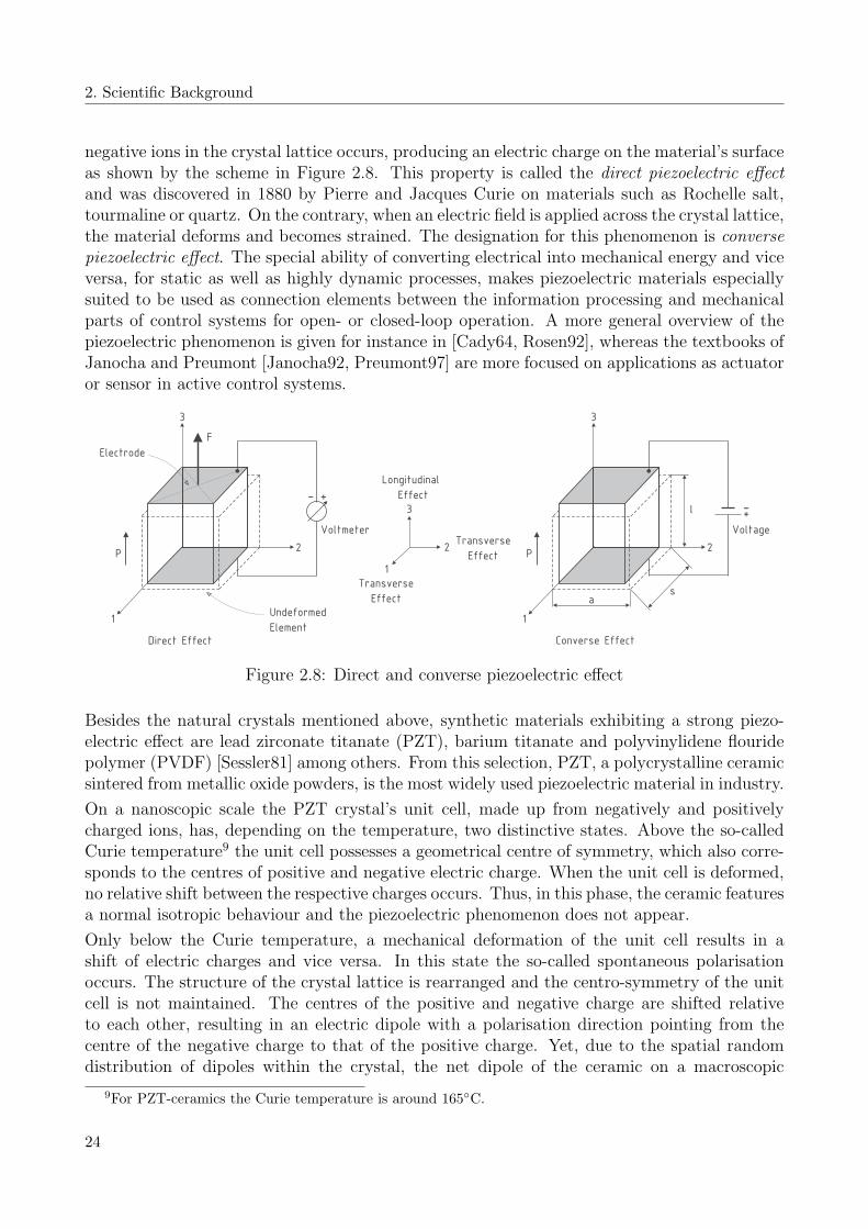
2. Scientific Background
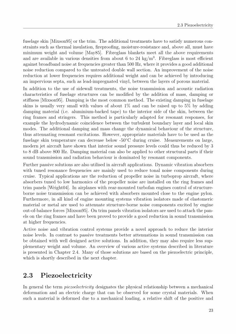
negative ions in the crystal lattice occurs, producing an electric charge on the material’s surfaceas shown by the scheme in Figure 2.8. This property is called the direct piezoelectric effectand was discovered in 1880 by Pierre and Jacques Curie on materials such as Rochelle salt,tourmaline or quartz. On the contrary, when an electric field is applied across the crystal lattice,the material deforms and becomes strained. The designation for this phenomenon is conversepiezoelectric effect. The special ability of converting electrical into mechanical energy and viceversa, for static as well as highly dynamic processes, makes piezoelectric materials especiallysuited to be used as connection elements between the information processing and mechanicalparts of control systems for open- or closed-loop operation. A more general overview of thepiezoelectric phenomenon is given for instance in [Cady64, Rosen92], whereas the textbooks ofJanocha and Preumont [Janocha92, Preumont97] are more focused on applications as actuatoror sensor in active control systems.
1
2
3
+-
Voltage
1
2
3
Undeformed
Element
+-
F
Voltmeter
a
Direct Effect Converse Effect
P
Electrode
Longitudinal
Effect
Transverse
Effect
Transverse
Effect
l
s
P
3
1
2
Figure 2.8: Direct and converse piezoelectric effect
Besides the natural crystals mentioned above, synthetic materials exhibiting a strong piezo-electric effect are lead zirconate titanate (PZT), barium titanate and polyvinylidene flouridepolymer (PVDF) [Sessler81] among others. From this selection, PZT, a polycrystalline ceramicsintered from metallic oxide powders, is the most widely used piezoelectric material in industry.
On a nanoscopic scale the PZT crystal’s unit cell, made up from negatively and positivelycharged ions, has, depending on the temperature, two distinctive states. Above the so-calledCurie temperature9 the unit cell possesses a geometrical centre of symmetry, which also corre-sponds to the centres of positive and negative electric charge. When the unit cell is deformed,no relative shift between the respective charges occurs. Thus, in this phase, the ceramic featuresa normal isotropic behaviour and the piezoelectric phenomenon does not appear.
Only below the Curie temperature, a mechanical deformation of the unit cell results in ashift of electric charges and vice versa. In this state the so-called spontaneous polarisationoccurs. The structure of the crystal lattice is rearranged and the centro-symmetry of the unitcell is not maintained. The centres of the positive and negative charge are shifted relativeto each other, resulting in an electric dipole with a polarisation direction pointing from thecentre of the negative charge to that of the positive charge. Yet, due to the spatial randomdistribution of dipoles within the crystal, the net dipole of the ceramic on a macroscopic
9For PZT-ceramics the Curie temperature is around 165C.
24
2.3 Piezoelectricity
scale is still zero and the material does not show a piezoelectric behaviour. Therefore, duringthe manufacturing process, the dipoles are aligned by applying a strong electric field to theceramic. This particular poling process leads to a remanent polarisation on a macroscopicscale and remains after the sintering process and removal of the poling field. As long as theceramic is not exposed to extreme temperature, electric or mechanical loads, the materialremains permanently piezoelectric and can be used to convert electric to mechanical energy orvice versa.
In a poled material like PZT, the piezoelectric behaviour is orthotropic with respect to thepoling direction P (see Figure 2.8). Assuming that the material is poled in the direction ofthe 3-axis and a positive electric field is applied along the same axis, the material will expandin direction of the electric field by ∆l and shorten in the plane normal to the field by ∆s and∆a. The designations for these phenomena are longitudinal and transverse effect. Both willalways appear conjointly and can be described by the following linear relations between thedisplacement and the voltage U applied across the electrodes in the poling direction:
Longitudinal effect: ∆l ∼ Eel · l = U , (2.62)
Transverse effect: ∆s ∼ Eel · s =s
l· U . (2.63)
The transverse effect is also observed in the 2-direction, hence ∆a ∼ Eel · a = a · U/l. Theterm Eel denotes the resulting electric field strength and is defined as the ratio of voltage U tothe ceramic thickness l in the 3-direction. This particular interaction between mechanical andelectrical quantities has to be taken into account when examining the mechanical behaviour ofthe piezoelectric continuum. A number of assumptions are made to derive the basic governingequations:
• In principle, the behaviour of a piezo ceramic is non-linear due to hysteresis and saturationeffects within the material. For the present application, it is assumed that non-linearitiescan be neglected. Depolarisation due to mechanical, thermal or electrical overloads mustbe prevented.
• Pyroelectric10 and thermal effects are not taken into account, as it is assumed that thematerial is exposed only to small temperature variations.
The mechanical behaviour of a linear elastic material placed in a zero electric field is describedby Hooke’s law:
ǫ = S · σ , (2.64)
where ǫ and σ are the vectors containing the strain and stress state of the elastic body. Strainand stress state are coupled through the compliance matrix S of the material.
In a stress-free dielectric medium the relation between the electric flux density D (electriccharge per unit area) and the electric field strength Eel is given by:
10An electric charge resulting from a temperature variation and vice versa.
25

2. Scientific Background
D = ε · Eel . (2.65)
Both quantities are coupled by the matrix ε, which is composed of the material’s dielectricpermittivity constants. The permittivity is often expressed in relation to the one of vacuum,which is ε0 = 8, 85 · 10−12 F/m.
For a piezoelectric material both types of behaviour are coupled according to the followingrelationship:
ǫ = S · σ + dT · Eel , (2.66)
D = d · σ + εσ · Eel . (2.67)
Equation 2.66 provides the basis to describe the application as actuator, whereas equation 2.67represents the sensor configuration. In matrix notation, they can be rewritten as:
(ǫD
)=
[SE dT
d εσ
]·(
σEel
). (2.68)
The matrix d contains the piezoelectric charge coefficients describing the amount of straininduced by an electric field in an unstressed material or the amount of electric flux densitycreated by a mechanical stress in a zero electric field. εσ is the permittivity matrix for aconstant stress state, whereas SE denotes the mechanical compliance matrix for a constantelectric field. In a Cartesian coordinate system, as illustrated in Figure 2.8, the strain andstress vector ǫ and σ, the electric flux density D and field strength Eel given in equation 2.68are defined as:
ǫ =
ǫ11ǫ22ǫ33
2 · ǫ232 · ǫ312 · ǫ12
, σ =
σ11
σ22
σ33
σ23
σ31
σ12
, D =
D1
D2
D3
, Eel =
Eel,1
Eel,2
Eel,3
. (2.69)
With the assumption of a poling along the 3-axis, the coupling matrix d and the dielectricmatrix εσ for a constant stress state take the following forms:
d =
0 0 0 0 d15 00 0 0 d15 0 0d31 d31 d33 0 0 0
, (2.70)
and
εσ =
εσ11 0 00 εσ
11 00 0 εσ
33
. (2.71)
26

2.3 Piezoelectricity
The first index used for the components of the coupling matrix refers to the axis of the electricfield and the second one to the considered mechanical degree of freedom. Thus, the term d31
corresponds to the transverse effect and d33 to the longitudinal effect. Similarly there exists ashear effect d15, when an electric field is applied along the 1- or 2-axis of the piezo. For thematrix εσ, the first index denotes the direction of the electric flux density and the second onethe direction of the applied electric field.
The components of the elastic compliance matrix SE for a constant electric field can be ex-pressed by the material properties in terms of Young’s moduli E, shear moduli G and Poisson’sratios ν, resulting in the expression:
SE =
1/E11 −ν12/E11 −ν13/E11 0 0 0−ν12/E11 1/E11 −ν13/E11 0 0 0−ν13/E11 −ν13/E11 1/E33 0 0 0
0 0 0 1/G23 0 00 0 0 0 1/G23 00 0 0 0 0 2 · (1 + ν12)/E11
. (2.72)
Nowadays, both the direct and converse piezoelectric effect are applied to a wide range oftechnical applications, ranging from audio buzzers as used in diverse electronic devices overquartz watches, microphones and accelerometers to ultrasonic transducers. For the purposeof active control the piezoelectric effect is either used in a sensor or actuator configuration.In this domain, PZT-ceramics and PVDF-foils are the most common piezoelectric materials.Some exemplary properties are listed in the table below. For comparison Barium Titanate andQuartz are also mentioned.
Table 2.1: Piezoelectric properties of PZT-5H, PVDF, Barium Titanate and Quartz
PZT PVDF Barium Titanate Quartz
Piezoelectric constant d31 [m/V]: −274 · 10−12 23 · 10−12 −35 · 10−12 ∗
Piezoelectric constant d33 [m/V]: 593 · 10−12 −33 · 10−12 86 · 10−12 ∗
Relative permittivity εσ11
/ε0 [-]: 3130 n/a 2920 4,52
Relative permittivity εσ33
/ε0 [-]: 3400 12,4 168 4,68
Density [kg/m3]: 7500 1800 6020 2650
Young’s modulus [N/m2]: 6, 0 · 1010 2, 0 · 109 1, 2 · 1011 7, 8 · 1010
Max. tensile strain [%]: 0,13 ≈ 50 n/a ≈ 0,2
Max. electric field [V/mm]: 1000 3 · 104 n/a n/a
Curie temperature [C]: 195 100 ≈ 120 583
∗ Piezoelectric coupling matrix d for Quartz: d11 = −2, 3 · 10−12 m/V, d14 = −0, 67 · 10−12 m/V,d26 = 4, 6 · 10−12 m/V, d12 = −d11 and d25 = −d14. The remaining terms are equal to zero.
On closer examination of the material’s relative properties, it becomes clear to what purposeeach type is adapted. Compared to PZT, PVDF-foils exhibit relatively small piezoelectricconstants as well as a low density and a low Young’s modulus. For this reason, the efficiencyof PVDF in converting electrical to mechanical energy is not very high and the use as anactuator on typical engineering structures is not very suitable. Nevertheless, the low stiffness,
27

2. Scientific Background
low weight and high tensile strength particularly enables PVDF-foils to be used as sensor.Possible applications can be found in [Henrioulle03, Lee90, Lee91].
PZT ceramics are commonly used in commercially available actuators and sensors. The mainactuator types are the stacked design and the laminar patch, which use the d33- and thed31-piezoelectric effect, respectively. Usually the longitudinal effect is twice as large as thetransverse effect and is the preferred design, as a greater amount of force can be generated inthis configuration. However, especially in the field of active structural acoustic control, thepiezo patch configuration has some advantages and is often used. The basic principles for thestacked design and laminar arrangement are presented in the following sections. Alternativedesigns are hybrid and shear actuators. In hybrid actuators an integrated motion amplifierincreases the limited actuator stroke in favour of the generated force [Janocha92, Rapp96]. Theamplifying mechanism is mostly based on the leverage principle or on flexural devices takingadvantage of the ratio between the longitudinal and lateral displacements in beam-like solidmaterials. An implementation of such a system has been realized for the actuation of higherharmonic control flaps in helicopter blades [Lorkowski01]. Designs using the shear deformationperpendicular to the electric field also reveal a great potential, since the shear effect d15 isapproximately equal to d15 ≈ d33 + |d31|. Though, due to the complex manufacturing process,a commercial application is still challenging to implement and to realise [Rapp96].
Actuator Stack Design
Actuators in stack design make use of the d33-effect. Since the maximum expansion in tensioncan only reach values in the order of 0,1 to 0,13% for typical PZT-ceramics, large actuatordimensions are required to achieve a reasonable stroke. However, this configuration wouldrequire high driving voltages to obtain an adequate electric field through the length of theactuator. For this reason stack actuators are made from a number of stacked, thin piezoceramicdiscs. The discs are separated by interjacent electrodes and paired in couples having an oppositepoling direction P as illustrated by the scheme in Figure 2.9. With this particular arrangement,the displacement of each single element is additive and a relative low voltage is sufficient togenerate the required electric field within each individual layer. To compensate the low tensilestrength of PZT-ceramics, a compression preload is usually induced in the actuators.
Interposed Electrode
+-Voltage
Piezo Stack
Idealized
Host Structure
Stiffness khs
Built-In Configuration
1
2
3Undeformed
Element
P
Piezo Layer
Figure 2.9: Piezoelectric stack actuator
The behaviour of a stack actuator can be described approximately with a simple static model.
28
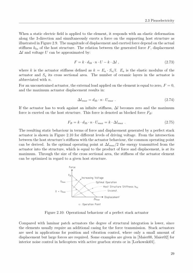
2.3 Piezoelectricity
When a static electric field is applied to the element, it responds with an elastic deformationalong the 3-direction and simultaneously exerts a force on the supporting host structure asillustrated in Figure 2.9. The magnitude of displacement and exerted force depend on the actualstiffness khs of the host structure. The relation between the generated force F , displacement∆l and voltage U can be approximated by:
F = k · d33 · n · U − k · ∆l , (2.73)
where k is the actuator stiffness defined as k = Ea · Sa/l. Ea is the elastic modulus of theactuator and Sa its cross sectional area. The number of ceramic layers in the actuator isabbreviated with n.
For an unconstrained actuator, the external load applied on the element is equal to zero, F = 0,and the maximum actuator displacement results in:
∆lmax = d33 · n · Umax . (2.74)
If the actuator has to work against an infinite stiffness, ∆l becomes zero and the maximumforce is exerted on the host structure. This force is denoted as blocked force FB:
FB = k · d33 · n · Umax = k · ∆lmax . (2.75)
The resulting static behaviour in terms of force and displacement generated by a perfect stackactuator is shown in Figure 2.10 for different levels of driving voltage. From the intersectionbetween the host structure’s stiffness with the actuator behaviour, the common operating pointcan be derived. In the optimal operating point at ∆lmax/2 the energy transmitted from theactuator into the structure, which is equal to the product of force and displacement, is at itsmaximum. Through the size of the cross sectional area, the stiffness of the actuator elementcan be optimized in regard to a given host structure.
Force
Displacement
Increasing Voltage
Host Structure Stiffness khs
FB
Umax
Dlmax
U=const.U < Umax
: Operation Point
Optimal Operation
Figure 2.10: Operational behaviour of a perfect stack actuator
Compared with laminar patch actuators the degree of structural integration is lower, sincethe elements usually require an additional casing for the force transmission. Stack actuatorsare used in applications for position and vibration control, where only a small amount ofdisplacement but large forces are required. Some examples are given in [Maier00, Maier02] forinterior noise control in helicopters with active gearbox struts or in [Lorkowski01].
29

2. Scientific Background
Laminar Patch Actuator
Laminar patch actuators are made from flat ceramic plates, which are bonded to the surfaceof the host structure or directly integrated into it. They are driven in the transverse modeand when an electric field is applied to the electrodes in 3-direction, the element respondswith an expansion or contraction along the 1- and 2-axis due to the d31-effect as shown inFigure 2.11. Because the displacement in this plane is partially constrained by the stiffnessof the host structure, in-plane forces and moments are generated and introduced into thestructure. Reciprocally, piezoelectric patches are also used in a sensor configuration, since astructural deformation inducing a strain in the plane of the elements can be measured throughthe resulting electric flux density D3.
1
2
3
Undeformed
Element
P
Piezo Patch
+-
Voltage
Built-In Configuration
Host Structure
Piezo Patch
Figure 2.11: Piezoelectrical patch actuator
Applied to typical lightweight structures as thin plates, the bending moments induced bythe actuator patch will generate an out-of-plane displacement of the plate. Since out-of-plane vibrations are also associated with the radiation of sound from plate-like structures,piezoelectric patches are especially suited to be used as actuators or sensors for active structuralacoustic control of lightweight structures. This bending principle can be realized in a so-calledbimorph or unimorph design. Both configurations are illustrated in Figure 2.12.
Piezo Patch
Strain Field
P U
P U
Unimorph ConfigurationBimorph Configuration
Symmetric Excitation
Bimorp Configuration
Assymmetric Excitation
P U
P U
P U
: Moment
: Force
Host
Structure
+
-
Figure 2.12: Configurations for surface bonded patch actuators
In the bimorph configuration the two opposed sides of the supporting plate are fitted withactuators patches, resulting in a symmetrical construction. If the actuators are poled in thesame direction, an electric field, having opposite signs on both sides, will generate a pure
30

2.3 Piezoelectricity
bending of the structure. The resulting extension in the neutral fibre is equal to zero becausethe opposed stresses generated by the upper and lower actuator are compensated by eachother. On the contrary, if the electrical field has the same magnitude and direction in bothactuators, a pure in-plane extension of the structure is obtained, as the strain field excited bythe actuators is symmetrical with respect to the plate’s neutral fibre.
In the unimorph configuration, only a single side of the structure is fitted with an actuatorpatch. Thus, simultaneously a bending moment and an in-plane force are induced into thehost structure.
An analytical model for the description of multi-layer laminates with integrated patch actuatorsis presented in Chapter 3.2. If the patches are used in a sensor configuration, the measuredelectric charge Q is equal to the integral of the electric flux density D3 over the electrodesurface. For an elastic beam of width b(x) and constant thickness h, on which is bonded asurface piezo sensor of negligible thickness and length l, the charge Q can be expressed withequation 2.67 for short-circuited electrodes, Eel = 0:
Q =
∫
l
D3 · b(x) · dx = −Ea · h/2 ·∫
l
d31 · w′′(x) · b(x) · dx . (2.76)
In this expression the strain has been replaced with the beam’s curvature w′′(x), since for thethin piezo layer the strain can be approximated by ǫ11 = −h/2 · w′′(x). The resulting chargeis proportional to a voltage USensor and might be measured via a current or charge amplifier:
USensor = −R · I = −R · Q = −QC, (2.77)
where R and C are the resistance and capacity of the current and charge amplifier respectively.
Compared with stack actuators, a higher stroke can be realized with the bending principle,but the stiffness and blocked force are usually considerably lower. As it is possible to bond thepatches directly onto the structure, the degree of structural integration is higher.
2.3.1 Thunder Actuators
For the design of the active trim panel attachment system piezoelectric Thunder actuators11
are used. Thunder actuators are small, adaptable and ready-made smart elements manufac-tured by Face International Corporation12 and available in a wide variety of configurationsand sizes. Through a special combination of materials and manufacturing process Thunderelements benefit from an exceptional ruggedness and can provide larger displacements thanother available piezoelectric actuators.
The operational mode of such an element is based on the piezoelectric d31-effect and the bendingprinciple presented in the previous chapter. Two typical Thunder elements are shown on theleft side of Figure 2.13. They are made from a composite laminate, consisting of a stainlesssteel substrate layer, a LaRCTM-SI layer13, a PZT piezoceramic wafer, another LaRCTM-SIadhesive layer and a thin aluminium or copper top layer (see exploded view in Figure 2.13)
11Thunder is an acronym for Thin Layer Unimorph Ferroelectric Driver.
12Face International Corporation, Norfolk, VA USA 23508, http://www.faceco.com/13LaRCTM-SI is a NASA patented high temperature polyamide adhesive.
31

2. Scientific Background
and are formed when the composite laminate is heated beyond the glass transition temperatureof LaRCTM-SI and cooled down to room temperature. During the cooling cycle, the material’sdifferent coefficients of thermal expansion induce a pre-stress in the individual layers leadingto the characteristic domed shape of the Thunder element.
Metal substrat
(stainless steel)
Adhesive layer
Adhesive layer
Piezoceramic (PZT)
Metal top
(aluminium or copper)
Figure 2.13: Thunder actuator and construction
As a result of the manufacturing process the internal stress state is such that the substrateis in tension and the ceramic in compression. This compression pre-stress for the PZT layerallows the element to be deflected far more than conventional piezoceramics without cracking.The metallic substrate layer and superstrate top layer also serve as electrodes for the electricpower supply.
The following figure illustrates the principles of Thunder operation by showing the typicalmotion versus the applied voltage. When no voltage is present, the piezoceramic materialremains in its pre-stressed compressive state while the steel substrate is in a tensile state asdescribed above. This condition is depicted in the middle of Figure 2.14.
++ --
Figure 2.14: Thunder motion for a simply supported device
With a positive electric potential applied to the electrodes, the d31-effect will try to shortenthe piezoceramic geometrically. This causes the stainless steel substrate to flatten and movedownward as illustrated on the left side of Figure 2.14. When a negative electric potential isapplied across the electrodes of a Thunder element the piezoceramic material geometricallyexpands, causing the Thunder to move upwards in order to accommodate for the increasedlength of the ceramic material. The voltage limits in the down direction are twice as large asin the up direction (2360 V/mm instead of -1180 V/mm), whereas the peak-to-peak voltageduring operation should not exceed 2360 V/mm. The operating temperature band ranges from-40 to 200C. Typical dimensions for rectangular Thunder elements may vary approximatelyfrom 20 by 10 mm to 75 by 50 mm, while using 0,2 mm up to 0,5 mm thick ceramic layers.Typical bidirectional displacements, which are achieved in a cantilevered configuration with
32

2.4 Active Control Technologies
the maximum allowable input voltage driven under 1 Hz, range from 0,1 mm to around 7 mm.The blocked force, measured for a simply supported device driven at maximum voltage, isranging from several Newtons to more than 100 N.
For a good performance the actuator mounting and the force transmission are the most im-portant points to consider when designing an active system with Thunder elements. In acantilevered configuration large displacements may be achieved but, due to the low stiffnessinherent to this arrangement, the ability to work against an external mass or stiffness is notvery effective. Furthermore, besides the normal deflection, the actuator’s end tip will alsoexecute a small rotation due to the beam-like bending. Hence, the normal actuation force isalways combined with a moment, which may make the active control impossible in certaincases.
To achieve a unidirectional translatory motion, it is possible to mount the Thunder elements ina clamshell configuration as reproduced in the drawing shown in Figure 2.15. Two elements arefastened symmetrically at their ends with an adequate clamping device. This design enablesthe actuator ends to move freely in the plane of the element, whereas at the centre points ofeach Thunder element the bending due to the piezoelectric d31-effect causes an opposite normaldeflection, which can be used as actuation force. The global behaviour of such an actuatorunit is similar to the one of a stack actuator presented in the previous chapter.
Out-of-plane Actuator
Force and DisplacementThunder Element
Thunder Element
Clamping Device
Free In-plane Motion
Figure 2.15: Thunder elements in a clamshell configuration
By using this symmetric configuration, the individual displacement of each element in the stackis additive, whereas for the force there is no change compared to a single actuator. An electricinsulation between the devices is not required, because they will be contacting each other atthe substrate layer only, thus sharing a common electric ground.
2.4 Active Control Technologies
Active technologies represent attractive solutions for various problems encountered in the con-trol of noise and vibrations. Typically, as shown in Figure 2.16, active control systems consistof actuators, used to manipulate the particular waveform within the fluid or structure that isto be controlled, sensors to detect the primary excitations and a control unit generating theactuator driving signal from the error signal. From this follows an important characteristic of
33

2. Scientific Background
active systems, which is the need of an external, additional energy supply. Another distinc-tive feature of active control systems, especially arising in vibro-acoustic applications, is thatactuators and sensors are often distributed and highly integrated within the structure, thusrequiring an integral modelling and development approach.
Fluid /
Structure
Control
Unit
SensorsActuators
Primary Excitation
Figure 2.16: Active control system
The fundamental principle of active control is the destructive wave interference. By adding asecond waveform to a primary perturbation a cancelling of the overall amplitude is obtainedif the second waveform is of equal amplitude and opposite phase to the primary perturbation.In an active system this is done by monitoring the resulting waveform with appropriate errorsensors and adapting the actuators and the second, artificially generated waveform with thecontroller in such way that a cancellation or at least a reduction of the residual amplitude atthe sensor is achieved. The waveforms can either be structural displacements or variations insound pressure.
First patent applications in the field of active noise control were made by Henri Coanda[Coanda30, Coanda32] and Paul Lueg [Lueg33] in the early 1930s (Coanda already men-tioned a possible aircraft application), however the ideas were far in advance of the electron-ics technology required for practical noise control systems. Nearly twenty years later, Olson[Olson53a, Olson53b, Olson56] experimented with an electronic sound absorber to reduce thelow-frequency noise in aircraft or automobiles in the vicinity of the occupant’s head. His ar-rangement consisted of a microphone mounted in close proximity to the face of a loudspeakercone. The loudspeaker was driven to null the sound pressure at the microphone, thus cre-ating a quiet area around it. Further applications already described by Olson are electronicnoise reducing headsets, active noise reduction in ducts and electronic vibration reducers. Hisexperimental results were promising, but the electronics technology of his time was still notsufficiently advanced to enable implementation in useful applications. Conover’s application ofloudspeakers arranged around a noisy transformer was another early attempt at active noisecontrol [Conover55].
The real breakthrough of active technologies came only in the 1980s, taking advantage of thefast advancing development of effective digital signal processors (DSP), along with progress inthe field of control algorithms and the introduction of new smart materials like piezoelectricceramics, magnetostrictive materials or shape memory alloys, allowing the design of new typesof actuators and sensors. Nowadays, active control of noise and vibration is an intensive fieldof research and is, for instance, covered extensively in the textbooks of [Elliott01a, Fuller96,Hansen97, Kuo96, Preumont97]. An overview of various applications is given in the survey
34

2.4 Active Control Technologies
articles of [Guicking03, Lago02]. In regard to their respective application, active solutions maybe classified into active noise control, active vibration control and active structural acousticcontrol systems, as described in the following chapters. The main emphasis is given to aircraftrelevant applications. Further applications as in the field of flow control [Thomas02] are notconsidered here, as they are beyond the scope of this study. The basic control schemes usedin active noise and vibration control are briefly addressed in Chapter 2.4.3.
2.4.1 Active Noise and Vibration Control
In active noise control applications a sound field cancellation is typically obtained with electro-acoustical actuators. Loudspeakers, used as actuators, cancel a sound pressure disturbance,which might be measured, for instance, with microphone sensors. As a result of this quite simpleprinciple, a zone of quiet is created in the near field around the sensor, whereas elsewhere thesound pressure level might also be increased due to constructive interference effects. Even so, amore detailed analysis, as given for example in [Mangiante77, Nelson92], reveals that in theoryit is possible to obtain a global attenuation inside a control volume without altering the soundpressure outside that volume by using a particular, continuous distribution of cancellationsources located on the surface of the controlled volume. However, a practical implementationwould involve a very high system complexity, thus limiting its practical relevance.
For this reason practical ANC solutions are restricted to systems where the wavelength at thehighest frequencies of interest is large with respect to the dimensions in which noise is to becancelled. In this particular case the spatial sound pressure distribution is nearly constantand a loudspeaker placed near the primary source acts as sound absorber. The best knownimplementations of this technique are ANC headsets, which are manufactured for instanceby trademarks such as Bose and Sennheiser for aircraft pilots. A further, commercial ANCsolution is available from Ultra Electronics in England and is used for quietening cabins ofturboprop aircraft with respect to low-frequency tonal noise components. It is fitted as astandard feature on the Bombardier Q Series Dash 8, Saab 2000, as well as Raytheon BeechKing Air 350, and the system is optional on a certain number of other turboprop and evenbusiness-jet aircraft. The system components are concealed behind the aircraft trim. On theSaab 2000, for instance, 74 microphones are linked to a control unit, which in turn drives a totalof 32 loudspeakers mounted on the trim panels [Lago02]. Thus, a global noise reduction insidethe passenger cabin is obtained on low-frequency, tonal propeller noise components. Activeheadrests with integrated microphones and loudspeakers, as already suggested by Olson andMay, are another possibility to create a local attenuation around the head of a passenger.However, applications in cars and jet aircraft require the control of broadband perturbations.A possible design is reported in [Rafaely99]. Such a system is also offered by Ultra Electronicsas Ultra Quiet Seat and is addressed to wide-bodied jet aircraft. It is reported to provide localbroadband attenuations of up to 10 dB.
Further examples of ANC solutions can be found for instance in duct acoustics applications,where it is possible to attenuate the low-frequency sound radiation emanating from air condi-tioning ducts, pipes, chimneys or exhausts [Kuo96, Lago02, Nelson92].
Vibration control is required on a wide variety of relevant engineering problems, either for struc-tural safety reasons or to guarantee the proper functioning of technical equipment and provideisolation from a vibrating environment. This can be handled either by passive techniques or
35

2. Scientific Background
by active vibration control. AVC differs from ANC that instead of sound pressure variationsstructural displacements, velocities or accelerations are controlled. To generate the necessarysecondary signals, force transducer elements such as electrodynamic shakers or piezoceramicmaterials are required, whereas elements allowing a monitoring of structural deformations andvibrations are used as sensors.
Typical AVC applications are developed for the implementation in lightweight structures asencountered on aircraft and spacecraft. In helicopters vibrations are generated from the tran-sient aerodynamic rotor forces at the blade-passing frequency and its harmonics. The vibra-tions are transmitted across the gearbox and the airframe to the pilot and the passengers.With active hydraulic actuators, replacing the conventional, elastomeric gearbox mounts, anaverage vibration reduction of up to 82% was demonstrated in flight tests [Fuller96]. For usein space applications various active systems have been designed to isolate antennas, payloads,technical equipment and experimental rigs from low-frequency structural vibrations. Someexamples are given in [Bushnell97, Collins91, Henderson96, Hyde97, Thayer99]. Furthermore,AVC techniques are also used in civil engineering and machine tool applications. For instanceactive tuned mass dampers acting as resonance absorbers are used in high buildings to reducewind-induced low-frequency vibrations. Active systems for the control of large cable struc-tures (bridges, antennas) are currently under development [Achkire97, Bossens01, Kubo04].In [Denkena04] a machine tool application to reduce chatter marks resulting from a relativemotion between the cutting tool and the workpiece is presented. An active vibration controlimplementation for circular saws is reported in [Chen03].
2.4.2 Active Structural Acoustic Control
The principle of active structural acoustic control represents a combination of both the ANCand AVC principles. In many relevant technical applications, as for instance car or aircraftinteriors, noise is primarily transmitted and radiated by the surrounding vibrating structure.Instead of controlling directly the sound pressure field and imposing a secondary, loudspeaker-generated sound field, the vibration characteristic of the structure itself is modified by thecontrol, thereby altering its radiation efficiency and attenuating its sound radiation behaviour[Fuller92]. As in AVC applications, structural actuators and sensors related to the sound pres-sure are used (microphones, acceleration or strain sensors). However, the controlled frequencyrange is typically much higher than in AVC applications. Advantages of ASAC in comparisonto ANC are that for some applications, involving for instance structural sound transmission,less control channels are required, thus reducing the system complexity. Furthermore, the actu-ator hardware implementation requires less weight and volume when strain-inducing actuatorssuch as piezoceramic elements are used.
A considerable amount of studies involving active structural acoustic control were publishedduring the last 15 years, documenting the advances made in the field of structural actuation,error sensing and control algorithms as well as the enormous interest of the research communityand industry in this area. In practice most vibro-acoustic relevant structures, as encounteredfor instance in cars or aircraft, consist of more or less flat single and double wall partitions.For this reason many ASAC publications address various theoretical and experimental aspectsin the control of sound transmission through general, flat homogeneous structures. The mainresults are summarized in the following two sections for single and double wall partitions.
36

2.4 Active Control Technologies
Some examples of prototype ASAC applications developed for more realistic structures suchas complete airframes are listed at the end of this chapter.
Control of Sound Transmission through Single Wall Partitions
The basic principles of active structural acoustic control are summarized in [Fuller96]. Consid-ering as example a theoretical model (rectangular single wall structure excited by plane wavesor local structural force inputs, a cost function related to the observed far field pressure isminimised with several independently controlled point forces or piezoelectric actuators), it isshown that, assuming certain conditions as proper size, number and placement of actuators,a reduction in sound transmission is achieved by two different control mechanisms: modalsuppression (also referred to as modal damping) and modal restructuring. Modal suppressionmeans that the excitation of structural modes having high radiation efficiencies is suppressedby the control, thus also attenuating the structural sound radiation. In contrast to this typeof control, which effectively reduces the mean vibration level of the structure, the modal re-structuring mechanism is based on the excitation of additional modes in such a way that theoverall radiation behaviour of the structure becomes less efficient due to a destructive infer-ence between the contributing radiation modes. However, with this type of control, the overallvibration level of the structure may not be attenuated significantly and sometimes even anincrease is noticed.
In [Wang91] a comparison is made between point force and piezoelectric actuators. The analysisreveals that with a point force control slightly better results in sound transmission attenuationare obtained. However, due to their low cost and light weight, the use of piezoelectric actuatorsis regarded as more suitable for practical implementations. The use of a point force actuatorfor the control of structural sound transmission into a closed cavity is addressed in a seriesof articles by Pan and Hansen [Pan90, Pan91a, Pan91b]. An electromagnetic driver is usedto minimise the sound pressure sensed by an error microphone in the cavity. Depending onthe excitation frequency, modal suppression and modal restructuring are identified as controlmechanisms. Furthermore, it is shown that the maximum noise reduction depends on theactuator location and that for an optimal system design additional constraints as the requiredactuation effort and resulting structural vibration level have be taken into account. A suc-cessful experimental application of piezoelectric actuators in the control of structural soundtransmission, also using microphone error signals, is described in [Clark92a].
Particular emphasis in literature is given to the sensing approach. For the structural integrationand from a practical point of view, it is desirable to have sensors located directly on thevibrating structure (acceleration and velocity sensors or strain-sensing elements as PVDF-foilsor fibre optic sensors) instead of using microphones. To obtain a satisfactory reduction in soundtransmission the physical quantities measured on the structure must provide a good estimateof the radiated sound power. As structural eigenmodes have different radiation efficiencies,this can be achieved either by designing distributed sensors, which respond only to certainstructural vibrations having a high radiation efficiency or by weighting the outputs from anarray of point sensors with an appropriate filter [Elliott93]. A control strategy, where the soundradiation is monitored with the strain field at discrete points on the structure, is proposed byMasson et al. [Masson97].
An active control of sound radiation using volume velocity cancellation is suggested by Johnson
37

2. Scientific Background
and Elliott [Johnson95], as in particular at low frequencies the most efficiently radiating velocitydistribution corresponds to the net volume displacement of the plate. This sensing strategyis compared in an analytical model to an optimal control where the radiated sound poweris minimised. It is shown that at low frequencies similar sound power reductions in the farfield are obtained with both types of control. However, volume velocity control is less proneto control spill-over 14 effects in terms of increased structural velocity and near-field pressureexcitation, when a reciprocal actuator to the volume velocity sensor, generating a uniform forcedistribution over the whole panel surface, is used.
The feasibility of implementing PVDF-foils as distributed error sensors on the radiating struc-ture is demonstrated with an experimental investigation in [Clark92b]. Two narrow PVDF-stripes are positioned perpendicular to each other on the supporting plate and thus measureodd plate-modes, which mainly contribute to the far-field sound radiation. Hence, the useof remote microphones in the control loop is not required. To detect the net volume veloc-ity of the radiating plate specially tailored PVDF-sensors, measuring the bending responseof the panel, are required. Experimental results obtained with such volumetric sensors arepresented in [Charette97b, Gardonio01, Henrioulle01]. However, practical implementationsare limited, as at higher frequencies the measured component related to an in-plane vibrationof the panel dominates the sensor response and interferes with the detection of the bend-ing components [Gardonio01]. An alternative approach to measure the volume velocity is itsapproximation by using the summed output from a number of discrete accelerations sensors[Elliott01b, Gardonio04a, Lee02].
In [Elliott01b, Gardonio04a] Elliott and Gardonio present a theoretical, comparative studycomprising various kind of embedded structural actuators and sensors. The actuation is madeeither via a single uniform force actuator or an array of piezoelectric patches, whereas forthe sensors a single volume velocity sensor or an array of point velocity sensors is used incombination with the actuators. The analysis is focused on systems based on single-channelfeedback controllers, either in a global SISO configuration or in a local MIMO configuration.It is reported that in terms of radiated sound power similar results are obtained with theglobal SISO and local MIMO system. However, some practical advantages are seen in theMIMO system, as a relatively large number of low-frequency resonant modes and their soundradiation as well as residual vibrations and therefore the near-field sound pressure can be moreefficiently controlled. The development and experimental testing of such a smart panel fittedwith 16 uniformly distributed and collocated acceleration-sensor piezoceramic-actuator pairsis described in a series of three papers presented by Gardonio, Bianchi and Elliott [Bianchi04,Gardonio04b, Gardonio04c]. Each local actuator sensor pair is driven by an independentsingle velocity feedback control loop, thus increasing the damping in the vicinity of resonancefrequencies. The experimental results prove that, provided an appropriate feedback gain ischosen, good reductions of the radiated sound power and the vibration energy of the panelcan be obtained for random primary excitations. Depending on the excitation type, shaker orloudspeaker, and its frequency, third octave band reductions in radiated sound power rangingbetween 5 and 8 dB are reported.
In the numerical study by Baumann and others [Baumann92] a pure vibration controller iscompared with a control system where the sound power, radiated from a beam and estimated
14The term spill-over designates the increased excitation with activated control on non-controlled quantitiesand frequencies.
38
2.4 Active Control Technologies
from filtered structural measurements, is minimised. Simulation results show that the acousticcontrol yields better results in terms of total radiated sound power than the vibration controller.At some frequencies an increase of structural vibrations is noticed with the acoustic controller asvibration modes with low radiation efficiencies are excited. For broadband excitations at higherfrequencies similar results are obtained with both sensing approaches. Baumann’s theory isalso investigated in [Thomas95], where a radiation filter matrix is used for the feedback controlof sound radiation from a simply supported plate excited by TBL noise. The results indicatethat a reduction of radiated sound power can be achieved on aircraft-like structures with anoptimal feedback control.
A real-time sensing procedure, intended to estimate the radiated far-field sound pressure ina given direction, was demonstrated theoretically and experimentally by Maillard and Fuller[Maillard94a, Maillard94b, Maillard95]. The system consists of several structural point sensors,such as accelerometers for instance, whose signals are post-processed by digital filters. Thefilters are designed to model the Green’s function between the sensors and a far-field location.The estimated far-field sound pressure is then used as an error signal in the ASAC system.The same authors present a numerical study [Maillard97] in which this sensing procedure iscompared to a technique where the net structural volume velocity is estimated from structuralpoint sensors. Using the same array of distributed acceleration sensors in both cases, theauthors conclude that better control performances can be obtained with an error signal basedon the estimated sound radiation.
Apart from the control strategy and type of actuators and sensors, the global control per-formance of ASAC systems is affected by additional parameters such as the number and sizeof actuators and sensors as well as their respective position on the structure. From a morepractical point of view, weight, power consumption and cost are further design variables to betaken into account.
Some intuitive design rules are given for instance in [Jakob99]. It is demonstrated with anumerical model that with each independent control force input one structural eigenmode of theplate can be controlled. This criterion determines the controllable frequency range, dependingon the number of actuators and sensors as well as the structural properties. Furthermore, astructural eigenmode cannot be controlled if the actuator or sensor is placed on a nodal line ofthis mode. It is shown that the optimal actuator location requiring the least actuation effortis in the antinodes of the associated eigenmode. Gardonio and Hansen [Gardonio04a] mentionthat, in general, the control performance in terms of sound power attenuation is increasedby employing a greater number of actuators and sensors. However, from a certain number ofactuators and sensors onwards, no major improvement is reached by a further increase in thenumber of control channels, which is explained by the physical spill-over effect introduced bypiezoelectric patch actuators having finite dimensions.
Due to the complexity of ASAC systems and the multitude of involved design variables, numer-ical optimisation techniques are proposed in literature. A general procedure for the design ofMIMO ASAC systems is suggested in [Clark92c]. Taking into account additional constraints asthe actuation effort, structural vibration levels, number and size of actuators, the optimisationproblem may become very complex. In such cases genetic algorithms (GA) prove to be a veryefficient optimisation technique. Some ASAC GA applications are described for instance in[Li04, Nijhuis03]. Further possible optimisation approaches are discussed in a review reportfrom Padula and Kincaid [Padula99].
39

2. Scientific Background
Control of Sound Transmission through Double Wall Partitions
Due to the fluid-structure coupling, double wall partitions have the particularity of not beingvery efficient in reducing the sound transmission at low frequencies. However, since ASAC ismost efficient in the lower frequency range, it is especially suited for reducing sound trans-mission through double wall partitions. Many aspects that hold for active control of soundtransmission through single wall partitions (main control mechanism, actuation, sensing, etc.)can also be directly applied to double wall partitions. Furthermore, some additional aspectsregarding the actuation and sensing approaches, which are unique to double wall sections, arediscussed in literature. In terms of actuation concepts the investigations can be divided intotwo main groups using either panel control or cavity control [De Man03]. Panel control is basedon structural actuators, whereas for cavity control acoustic sources located inside the doublewall cavity are used, thus blocking the airborne sound transmission path. For the error signaleither structural sensors or microphones located in the radiated sound field or in the cavity areused. However, similar to the literature available for single wall partitions, most authors treatonly homogeneous, flat panel systems.
A comparative study between the panel and cavity control concept is presented in [Bao97,Pan98a]. The authors conclude that a cavity control approach in combination with cavitypressure sensors yields a better control performance in terms of sound radiation and vibra-tion attenuation in comparison to a panel control approach. Similar results are obtained byDe Fonseca et al. in a numerical and experimental study addressing the sound transmissionthrough an aircraft sidewall consisting of a stiffened skin panel and a homogenous trim panel[De Fonseca98, De Fonseca99]. This behaviour can be explained by the fact that in the con-sidered frequency range the modal density in the uncoupled cavity is usually much lower thanon the uncoupled panels, which allows the use of less actuators and sensors with a cavitycontrol concept [De Man03]. Concerning the active control of stiffened double wall cylinders,comparable results are obtained in a numerical study by Grosveld [Grosveld96]. It should bementioned that these conclusion are only valid if, besides the airborne transmission path, noadditional structure-borne paths are present within the structural system.
An analytical and experimental study of active control of sound transmission through a doublewall system is presented by Carneal and Fuller [Carneal93, Carneal03]. The actuation is madevia a set of piezoelectric patches either applied on the incident or the radiating panel. A set ofmicrophones placed in the receiving chamber provide the error signal for the controller. Fromboth analytical and experimental results the authors conclude that active control applied tothe radiating panel is the more effective solution in terms of TL increase as this structuralconfiguration exhibits a more efficient coupling to the radiated sound field. In addition, it isreported that the use of a stiff radiating panel increases the passive transmission loss perfor-mance as well as the control performance achieved with the active system. The panel controlconcept in combination with a volume velocity sensor is investigated in an article by Pan et al.[Pan98b]. The main finding is that in contrast to single panels, as investigated in [Johnson95],the control efficiency is limited to approximately half of the frequency range. This behaviour isexplained by the modal participation of the first structural radiation mode, which is less dom-inant at higher frequencies in double wall systems than on a comparable single wall partition.To achieve a better active attenuation at higher frequencies the authors suggest the structuralcontrol of additional, low-order radiation modes.
40

2.4 Active Control Technologies
A further comparative study of panel and cavity control is given in [Maury01]. The articleaddresses the control of flow-induced sound transmission through a generic aircraft sidewall(using flat, homogenous panels without structure-borne sound transmission). From a numericalmodel it is concluded that for a significant noise reduction in the low-frequency range the mostefficient control strategy is the suppression of low-order skin panel modes. A less efficientcontrol performance is obtained by suppressing structural trim-panel modes, whereas with acavity control concept the least good sound attenuations are achieved.
Finally, a theoretical study concerning the active control of airborne and structure-borne soundtransmissions through an aircraft sidewall is presented in a paper by Gardonio and Elliott[Gardonio98]. The structural model consists of a skin panel stiffened by stringers. In contrastto the aforementioned studies the trim panels are coupled to the skin panel by the cavity fluidand structural attachment elements allowing an additional structure-borne sound transmission.Three different control concepts are investigated by the authors: active mounts connecting bothpanels and driven in such a way as to cancel the out-of-plane velocity on the trim panel orminimise the total radiated sound power, cavity control with loudspeakers cancelling the cavitysound pressure or minimising the total radiated sound power and a combination of both sys-tems. The control performance is evaluated for different cavity configurations (empty, partiallyor entirely filled with porous absorption material) and for transverse force and plane wave pri-mary excitations. The results suggest that a cavity control with loudspeakers provides goodattenuation in the mass-air-mass frequency range, whereas with active mounts no significantreduction of sound transmission is obtained, as in this frequency band the sound transmissionis largely dominated by the airborne transmission path. Similar conclusions can be drawn fromthe experimental study of De Fonseca et al. [De Fonseca99].
ASAC Applications
The first full-scale, laboratory ASAC application was carried out on a fully trimmed DouglasDC-9 aft section [Fuller96]. A harmonic engine excitation as due to engine out-of-balanceforces was simulated with a set of two shakers attached to the engine mounts and control wasperformed with two shakers, internally mounted to the engine pylon. Several combinations ofup to seven microphones and five acceleration sensors were used for the error signal. Withan acceleration control, local reductions in SPL of up to 9 dB were obtained at the excitationfrequency of 170 Hz. However, on some microphones increased sound levels were also ob-served with activated control, thus highlighting the already mentioned aspect of ASAC controlsystems that a minimisation of vibration energy does not necessarily guarantee a noise atten-uation. Also for a DC-9 engine mounting system a case study for active engine mounts basedon hybrid electromagnetic-hydraulic actuators was carried out. The system is reported tosignificantly reduce the structure-borne noise transmitted from the engines into the airframe,thus attenuating the global cabin noise, while the engine’s vibration level is not increased[Swanson93].
The reduction of propeller noise in turboprop aircraft by ASAC means is addressed in somestudies. Sollo et al. investigated the application of ASAC systems to the ATR aircraft family[Sollo98]. This approach was demonstrated on a ATR42/72 fuselage mock-up, which was fit-ted with piezoceramics patches bonded to the fuselage skin and frames. The error signal wasderived from microphones distributed inside the cabin at seated passenger height. The first
41
2. Scientific Background
three propeller tones were controlled simultaneously and average noise reductions of around10 dB were measured for the most significant test conditions. A flight test demonstration ofan operational ASAC system was conducted on a Raytheon 1900D, a 19-seat twin turbopropaircraft [Palumbo99, Palumbo00]. The control system consisted of 21 inertial force actuatorsmounted on the fuselage frames and 32 microphones located near the passenger’s head posi-tions. Interior noise reductions of up 15 dB at the blade-passing frequency of 103 Hz wereobtained during single-frequency control test, whereas on multi-frequency control tests at theBPF, its first and second harmonic, simultaneous reductions of 10 dB, 2,5 dB and 3 dB wereobtained.
An ASAC application for helicopters is currently under development in Germany. In helicoptersthe gearbox represents a principle source of interior noise. Vibrations at the dominant gear-meshing frequency of about 1,9 kHz are transmitted as structure-borne sound through thegearbox struts into the airframe and radiated into the cabin. A prototype ASAC system basedon smart gearbox struts with integrated piezoelectric actuators and acceleration control wassuccessfully demonstrated in flight tests. Mean reductions of about 11 dB have been obtainedfor the cabin SPL on the dominant frequency [Maier00, Maier02].
Control of sound radiation with adaptive tunable vibration absorbers (ATVA) is another tech-nique becoming increasingly popular for aircraft implementations [Carneal04, Charette97a,Franchek93, Wright04]. It is in fact a combination of passive and active methods. Basically,an ATVA works like a classical, passive vibration absorber, however the ATVA resonance fre-quency can be adjusted by active means in accordance with the operation conditions, thusincreasing the bandwidth and performance of control. In contrast to an active solution withconventional transducers (piezoceramic patches, shakers, loudspeakers, etc.), a much lowercontrol authority and system complexity is required and less electrical power is consumed.
2.4.3 Control Schemes
With respect to the utilised control laws, active control systems can be divided into feedforwardand feedback control schemes. The main difference between a feedforward control scheme andfeedback scheme is that with feedforward control a reference signal correlated to the actualprimary disturbance is required in addition to the error sensors, whereas with feedback systemsthe requirement of additional reference sensors is eliminated.
Both control schemes can be used in principle with random and deterministic excitations. How-ever, feedforward control of random excitations is only possible if the reference sensor is placedin a sufficient upstream direction with respect to the error sensors and the disturbance trans-mission. This limitation is due to the delay experienced with real-time control systems and istermed causality constraint [Burdisso93]. Thus, to guarantee a good control performance, thedelay in the control path from the reference sensor to the error sensors must be smaller thanthe time required for the primary disturbance to travel from the reference sensor to the errorsensors. Harmonic feedforward control requires only the detection of the fundamental driv-ing frequency. Due to its ease of implementation and relatively good stability properties, thefiltered-X least-mean-square (LMS) algorithm is a feedforward control scheme that is widelyused in experimental applications for the control of harmonic disturbances (see for instance[Carneal93, De Fonseca98, De Fonseca99, Maier00, Palumbo99, Sollo98]). In numerical inves-tigation LMS algorithms are also a very popular choice, as they give an upper-bound estimate
42

2.5 Conclusions
of the best possible control performance [De Fonseca98, De Man03, Gardonio98, Grosveld96,Nijhuis03].
However, the need for an additional reference signal represents a constraint for many practicalapplications and can be avoided by the use of appropriate feedback controllers. In model-basedfeedback control the control algorithm is reformulated internally as a feedforward problem byusing an internal model of the plant [Baumann92]. Yet, as the implementation of such model-based controllers is difficult, non-model-based feedback controllers, being easier to implementin practice, are often preferred in literature [De Man03]. A shortcoming associated with thistype of control is a limited control authority and performance since the system’s stability mustbe guaranteed for various operating conditions. Nevertheless, by using collocated actuator andsensor pairs, as for instance point force actuators and velocity sensors, stability robustnessis increased and as a result of the active control the damping in the structure is augmented[Preumont97].
In ASAC implementations this principle is frequently realized with collocated, uniform forceactuators and sensors based on PVDF-foils or piezoelectric patches in combination with ac-celeration sensors. Thus, with a direct velocity feedback control the sound radiation fromlightweight structures can be reduced, as the resonant components of the structural responseto the primary excitation are more efficiently damped [Elliott01b, Gardonio01, Gardonio04b,Henrioulle01, Johnson95, Lee02, Nijhuis03]. As previously mentioned, in some studies the useof multiple actuator and sensor pairs connected by independent, local velocity feedback controlloops is suggested in order to reduce structural sound radiation. This control configuration isreferred to in literature as decentralised velocity feedback control [Gardonio04a, Gardonio04c].
2.5 Conclusions
From the available publications on active structural acoustic control one can conclude that it ispossible to develop active control systems for reducing the sound transmission through singleand double wall structures. However, the multitude of possible approaches and results alsoillustrate that the complexity of such systems remains on a very high level, especially whenused in combination with double wall partitions. For these reasons it is important to considerall important factors affecting the control performance in the system design. These factorsare, amongst others such as the power consumption or desired system complexity, the specificdesign of the structure to which the ASAC system is to be applied (stiffened structure, airborneand structure-borne transmission paths, cavity absorption), the type and positioning of theactuators, the sensor concept (structural or acoustic sensors), the type of primary excitation(harmonic or random, force or acoustic excitation) and the controller design (feedback orfeedforward control scheme, narrow- or broadband excitation). In the present application thesystem development is based on a detailed numerical simulation model, which is presented inthe next chapter.
43

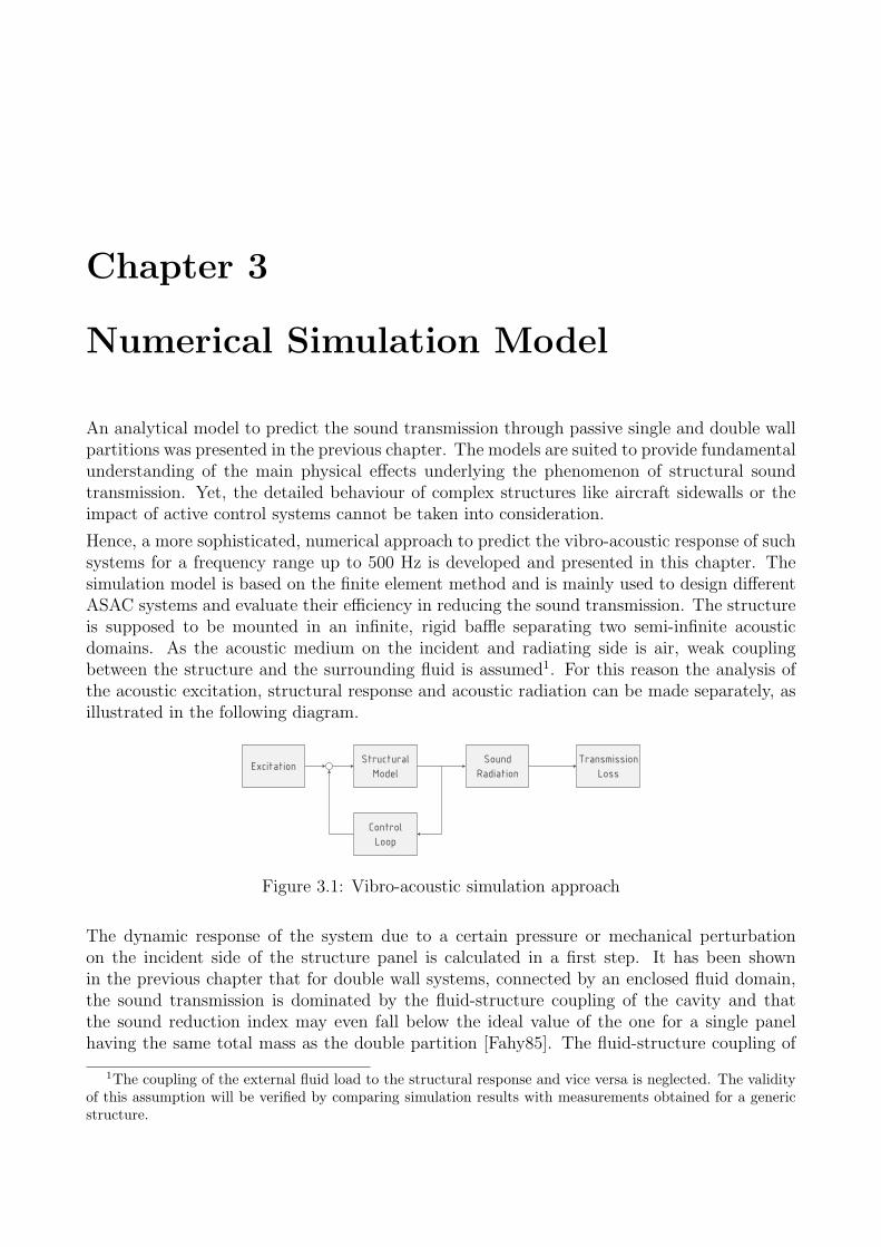
Chapter 3
Numerical Simulation Model
An analytical model to predict the sound transmission through passive single and double wallpartitions was presented in the previous chapter. The models are suited to provide fundamentalunderstanding of the main physical effects underlying the phenomenon of structural soundtransmission. Yet, the detailed behaviour of complex structures like aircraft sidewalls or theimpact of active control systems cannot be taken into consideration.
Hence, a more sophisticated, numerical approach to predict the vibro-acoustic response of suchsystems for a frequency range up to 500 Hz is developed and presented in this chapter. Thesimulation model is based on the finite element method and is mainly used to design differentASAC systems and evaluate their efficiency in reducing the sound transmission. The structureis supposed to be mounted in an infinite, rigid baffle separating two semi-infinite acousticdomains. As the acoustic medium on the incident and radiating side is air, weak couplingbetween the structure and the surrounding fluid is assumed1. For this reason the analysis ofthe acoustic excitation, structural response and acoustic radiation can be made separately, asillustrated in the following diagram.
Structural
Model
Control
Loop
Sound
RadiationExcitation
Transmission
Loss
Figure 3.1: Vibro-acoustic simulation approach
The dynamic response of the system due to a certain pressure or mechanical perturbationon the incident side of the structure panel is calculated in a first step. It has been shownin the previous chapter that for double wall systems, connected by an enclosed fluid domain,the sound transmission is dominated by the fluid-structure coupling of the cavity and thatthe sound reduction index may even fall below the ideal value of the one for a single panelhaving the same total mass as the double partition [Fahy85]. The fluid-structure coupling of
1The coupling of the external fluid load to the structural response and vice versa is neglected. The validityof this assumption will be verified by comparing simulation results with measurements obtained for a genericstructure.

3. Numerical Simulation Model
the enclosed cavity must be consequently fully taken into account by the structural model.Once the dynamic behaviour on the radiating parts of the structure has been determined, thefree field sound radiation is calculated with the Huygens-Rayleigh integral and the resultingtransmission loss index is derived.
The ASAC system is incorporated by additional control loops for each individual actuatorelement. As the structure and the surrounding acoustic medium can both be considered tohave a linear behaviour for small displacements, the superposition principle is used to computethe controlled system response, which will be a complex linear combination consisting of theprimary response due to the initial perturbation and weighted secondary, controller-generatedresponses.
A validation of the numerical simulation model and the assumption of a weak fluid-structurecoupling is presented at the end of this chapter. For a generic structure, consisting either ofsingle or double wall aluminium panels, numerical and experimental results are compared anddiscussed for the structural and acoustic domain.
3.1 Modelling of Structural Sound Transmission
In recent years numerical modelling of miscellaneous vibro-acoustic problems has become acommon subject in research and industry. The applications vary from diverse vehicle inte-rior acoustic problems [Barisciano99, Kropp03, Marburg03, Papadopoulos03, Peiffer05] to themechanical behaviour of complex structures (ships, satellites, etc.) coupled or excited by acircumjacent fluid [Cabos03, Moosrainer00, Witting99]. Depending on the type of analysis,the following numerical methods as well as suitable combinations are mainly used to solvevibro-acoustic problems:
• the finite element method (FEM),
• the boundary element method (BEM),
• and the statistical energy analysis (SEA).
The boundary element method is a numerical solution of the Kirchoff-Helmholtz wave equationand is used for radiation and scattering problems. In this formulation the sound field isrelated to the sound pressure and particle velocity on a closed boundary and additional soundsources. Closed and infinite fluid domains can be considered with this method. The SEA-method is based on the analysis of the mean energy equilibrium for a given system and on thebreakdown of average power flows between complex subsystems as for instance structural andfluid domains. The subsystems are excited by frequency bands rather than single harmonicfrequencies, which makes SEA especially suited to high-frequency problems with broadbandexcitation. Further information on the BEM- and SEA-methods are available for example in[Crighton92, Estorff00].
The present application involves the calculation of sound transmission through a generic side-wall partition consisting of several panels coupled by an enclosed fluid domain. As the fre-quency range is restricted to frequencies up to 500 Hz, and due to the additional requirementto incorporate the impact of piezoelectric actuators on the structural behaviour, an FEM-based simulation procedure is chosen to model the vibro-acoustic response of such a system.
46

3.1 Modelling of Structural Sound Transmission
The structural dynamic analysis is accomplished with the FEM-software MSC/Nastran andthe numerical tool Matlab is used for pre- and post-processing of the acoustic results and theimplementation of the control loop.
3.1.1 Structural Model
Real vibratory systems, having a continuous distribution of mass and stiffness, are character-ized by the fact that they possess an infinite number of degrees of freedom. Mathematically thisbehaviour leads to a description with partial differential equations, which might be solved an-alytical for simple structures. But in general, for complex structures and boundary conditions,an analytical solution is not possible anymore.
With the method of finite elements a standard numeric tool is available that can be used todescribe the static and dynamic behaviour of complex mechanical systems. The basic ideabehind the FEM-procedure is that the structure can be discretised into small finite elements,which can be described by piecewise-continuous simple solutions. Each element is coupled inits respective behaviour to adjacent elements by several boundary constraints, thus leadingto a global equation system combining the properties of the whole structure. By choosingan appropriate degree of discretisation and suitable types of finite elements, the structuralbehaviour can be predicted with an adequate accuracy. Formally this approach corresponds toa discretisation of the continuum and the partial differential equation is reduced to a systemof standard differential equations [Bathe82, Cook89, Moosrainer00].
Assuming linear-elastic material behaviour and small deformations the governing equation ofmotion for a structural frequency-response FEM-analysis is derived from the Lagrange equationand Hamilton’s Principle:
Ms · X(t) + Cs · X(t) +Ks ·X(t) = Rs(t) , (3.1)
in which X is the structural, nodal displacement vector with Ns degrees of freedom, Rs a struc-tural excitation, Ms the mass matrix, Ks the structural stiffness matrix and Cs the dampingmatrix.
Starting with the weak formulation of the wave equation the governing equation of motionused in a fluid domain FEM-analysis is:
Mf · P (t) + Cf · P (t) +Kf · P (t) = Rf (t) , (3.2)
where Mf is the acoustic mass matrix, Cf the acoustic damping matrix, Kf the acousticstiffness matrix, Rf an acoustic load and P the acoustic, nodal pressure vector ∈ R
Nf . Math-ematically equation 3.1 and 3.2 represent each a linear system of second order differentialequations.
Assuming a steady state solution of equation 3.1 the displacement vector can be written as:
X(t) = X(ω) · ejωt , (3.3)
where X(ω) denotes the complex amplitude at the angular frequency ω. Introducing equation3.3 and its time derivatives in equation 3.1 yields:
47

3. Numerical Simulation Model
[−ω2 ·Ms + jω · Cs +Ks
]· X(ω) = Rs(ω) , (3.4)
which is the governing equation of motion in the frequency domain. It can be solved by invertingthe matrix term [−ω2 ·Ms + jω · Cs +Ks] for each forcing frequency, which is referred to asthe direct approach. The fluid’s equation of motion may be solved in a similar way.
For systems possessing a large number of degrees of freedom and forcing frequencies a direct so-lution of equation 3.4 may not be very efficient from a computational point of view [Blakely93].An alternative solution is provided by a modal formulation, decoupling the equation of motion3.4.
Using the homogenous equation of motion without considering the damping term Cs and byassuming that the displacement vector can be written as:
X(t) = φ · ejωt , (3.5)
the solution for a free, undamped vibration is obtained by solving the eigenvalue problem:
[K − ω2 ·M
]· φ = 0 . (3.6)
Equation 3.6 can be resolved with the theory of eigenvalues resulting in exactly Ns eigenpairs oreigenmodes (ω1, φ1), . . ., (ωNs
, φNs), each satisfying the homogenous equation of motion for an
undamped, free vibratory system. φi is the eigenvector or mode shape and ωi the correspond-ing eigenfrequency. One can now define a matrix Φs, whose columns contain the orthogonaleigenvectors φi as well as a matrix Ωs containing the eigenfrequencies on the diagonal entries.
As the matrix of eigenvectors Φs defines a base of RNs , the complex amplitude X(ω) can
be expressed as a weighted superposition of eigenvectors, a formulation also known as modalexpansion in literature:
X(ω) = Φs · α(ω) . (3.7)
The vector α(ω) is the modal amplitude and describes the contribution of the different modeshapes to the structural displacement vector at a given forcing frequency ω. Multiplying theequation of motion with ΦT from the left and replacing the displacement X with its modalexpansion results in the following system of equation for the modal amplitude α(ω):
[−ω2ΦT
s MsΦs + jωΦTs CsΦs + ΦT
s KsΦs
]· α(ω) = ΦT
s · Rs(ω) . (3.8)
Φs can be mass-normalized such that ΦTs MsΦs = I and ΦT
s KsΦs = Ω2. A particular so-lution is obtained for undamped systems with Cs = 0. Due to the diagonal properties of[−ω2ΦT
s MsΦs + ΦTs KsΦs
]equation 3.8 is reduced to a system of Ns uncoupled equations, each
representing a single mass oscillator. However, in general the matrix ΦTs CsΦs is full and an
efficient solution of equation 3.8 is not possible anymore. But, with the presumption of a modaldamping as given by the following relation, the term ΦT
s CsΦs is reduced to a diagonal formand the benefits from the diagonal matrix properties in equation 3.8 are retained:
ΦTs · Cs · Φs = 2 · diag(ωiζi) . (3.9)
48

3.1 Modelling of Structural Sound Transmission
The variable ζi represents the modal damping parameter for the i-th eigenmode and is definedas ratio between the damping coefficient cj to the critical damping ccr,j characterizing theaperiodic solution of a single mass oscillator (cj, mj, kj being the damping coefficient, massand stiffness of the single mass oscillator):
ζi =cjccr,j
=cj
2 ·√kj ·mj
. (3.10)
The introduction of a modal damping matrix corresponds to the assumption that the com-plete energy dissipated during one vibratory cycle can be expressed as the sum of individualdissipation losses for each participating eigenmode. Typically, most engineering structures areweakly damped and the damping ratios that can be found in literature for various types ofstructures vary from 0, 5 up to 15% [Cook89, Cremer96]. The general solution of equation 3.8is then obtained by:
αj(ω) =φT
s,j · rs,j(ω)
ω2j + 2 · jω · ωj · ζj − ω2
, j = 1 . . . Ns . (3.11)
For a harmonic excitation, modes with an eigenfrequency much higher than the forcing fre-quency contribute in general only to a neglectable extent to the displacement given in equation3.7 and it is a common approach to truncate the modal expansion after the first M modes.Thus, the displacement vector is approximated by:
X(ω) ≈ Φs · α(ω) , (3.12)
with the reduced subspace Φs ∈ RNs×M and α(ω) ∈ C
M . Typically M ≪ Ns and the compu-tational effort in determining the modes and the modal amplitude is reduced to a great extentin comparison to the exact solution.
Applying the modal approach to the equation of motion valid for the fluid domain, results ina similar modal expansion for the complex pressure vector P (ω):
P (ω) = Φf · β(ω) . (3.13)
Φf is the matrix of acoustic eigenvectors and β(ω) the modal amplitude vector of the fluid.Once the sound pressure has been computed, the particle velocity is derived from the Eulerequation ∇p = −jω · ρf · v.When the structural behaviour is coupled to a fluid domain and vice versa the respectiveequations of motion 3.1 and 3.2 cannot be solved separately anymore. On the interface betweenthe structure and the fluid the boundary condition is given by:
∂p
∂n= −ρf ·
∂2xn
∂t2, (3.14)
with n as normal unit vector pointing from the wetted surface to the structure and ρf as fluiddensity. For the structure and the fluid equation 3.14 corresponds to additional exterior loadsapplied on the interface surface Ssf . The pressure load on the structure is:
Rs =
∫
Ssf
(NTX · n) · p · dS =
∫
Ssf
(NTX · n) ·NP · dS · P = L · P , (3.15)
49

3. Numerical Simulation Model
and the acoustic load due to the vibrating structure equals:
Rf = −∫
Ssf
NTP · xn · dS = −
∫
Ssf
NTP · (n ·NX) · dS · X = −LT · X , (3.16)
since L is the coupling matrix defined by:
L =
∫
Ssf
(NTX · n) ·NP · dS . (3.17)
NX and NP denote the interpolation matrices relating the discrete, nodal displacement andpressure vectors to the displacement and pressure distribution within one element.
Including the additional exterior loads on the left-hand side of equations 3.1 and 3.2 results inthe governing equation of motion for the coupled fluid-structure problem:
[Ms 0LT Mf
](X(t)
P (t)
)+
[Cs 00 Cf
] (X(t)
P (t)
)+
[Ks −L0 Kf
] (X(t)P (t)
)=
(Rs(t)Rf (t)
), (3.18)
which may be written in the frequency domain as:
[−ω2Ms + jωCs +Ks −L
−ω2LT −ω2Mf + jωCf +Kf
](X(ω)
P (ω)
)=
(Rs(ω)
Rf (ω)
). (3.19)
Replacing the vector P (ω) with Ψ(ω) as defined by the function P (ω) = jω ·Ψ(ω) and dividingthe second line of equation 3.19 with −jω yields a symmetric formulation of the coupledequation of motion:
[−ω2Ms + jωCs +Ks −jωL
−jωLT ω2Mf − jωCf −Kf
] (X(ω)
Ψ(ω)
)=
(Rs(ω)
−(jω)−1 · Rf (ω)
). (3.20)
A modal transformation is carried out analogously to equation 3.7 and 3.13 by using theuncoupled structural and acoustic modes φs and φf . The resulting coupled equation of motionin modal coordinates reads:
[−ω2ΦT
s MsΦs + jωΦTs CsΦs + ΦT
s KsΦs −jωΦTs LΦf
−jωΦTf L
T Φs ω2ΦTfMfΦf − jωΦT
f CfΦf − ΦTfKfΦf
]·
·(α(ω)ψ(ω)
)=
(ΦT
s Rs(ω)
−(jω)−1 · ΦTf Rf (ω)
), (3.21)
with ψ(ω) given by Ψ(ω) = Φf · ψ(ω).
In many applications such as double wall partitions an enhancement of the sound absorptioncapabilities is achieved by lining the fluid surface with elastic-porous absorbers as fibreglassor open-cell foam. The additional source of damping provided by those materials is included
50

3.1 Modelling of Structural Sound Transmission
in the fluid model by applying the Bliss boundary condition [Bliss82a] to the fluid-structureboundary:
Psf (ω) +B(ω) · ∇2sf Psf (ω) = Z(ω) · Vn(ω) . (3.22)
Psf (ω) and Vn(ω) are the surface sound pressure and normal particle velocity respectively. Theabsorber properties are defined in terms of their normal impedance Z(ω) and the bulk reactingcoefficient B(ω). The normal impedance is easily determined in a Kundt’s tube and a methodto measure the bulk reacting coefficient has been suggested by Bliss and Burke [Bliss82b].The operator ∇2
sf contains second derivatives in the plane of the surface and the whole term
B(ω) · ∇2sf Psf (ω) takes into account the additional sound absorption on a porous surface due
to velocity components in the plane of that surface.
By neglecting the bulk reacting coefficient or for normal incident sound waves, equal toB(ω) · ∇2
sf Psf (ω) = 0, the classical normal impedance boundary condition is obtained:
Z(ω) =Psf (ω)
Vn(ω). (3.23)
In this case, the sound absorption is governed only by the real part of the impedance and thedamping matrix Cf has contributions from the real part of the impedance and the stiffnessmatrix Kf contains contributions from the imaginary part of Z.
3.1.2 Structural Excitation
For the primary excitation of the structure, different concepts are used. One model is thoughtas a very simple approximation of a buzz-saw noise type excitation: a monopole source placedat the location of the engine inlet, radiating towards the fuselage with constant power at allfrequencies. This setup will allow testing the efficiency of the noise reduction system againsta tonal, coherent noise source. A diffuse sound field can be modelled by using plane wavesuperposition and a mechanical point force excitation can be used for simple test purpose orthe simulation of structure-borne sound as excited for example by engines due to rotating,unbalanced masses.
The single monopole source is located at a position r relative to the point of origin of thex,y,z-coordinate system, x and y being the axes in the panel plane and z the normal axis tothe panel as depicted in Figure 3.2.
To determine the excitation sound pressure level on the panel at a position rs the assumption ismade that the structure is totally rigid. Therefore, free field propagation can be assumed andthe pressure values obtained with the following equation must be multiplied with a factor oftwo in order to take into account the total reflection on the rigid surface. With the assumptionof a small source diameter a in comparison to the acoustic wavelength, 2π · a/λ ≪ 1, thecomplex, free field pressure radiated by a monopole source with the volume flow Q at theangular frequency ω is given by [Fahy85]:
p (rs) = jω · ρ0 ·Q
4π ·R · e−jωR/c0 . (3.24)
51

3. Numerical Simulation Model
Structure
z
x
y
dS
r R
rSn
Monopole Source
Figure 3.2: Acoustic excitation with a monopole source
The termR is the distance between the source and the observer point on the panel, R = |rs − r|.The volume velocity Q is equal to 4π · a2 · vn, with vn being the normal velocity of the source.ρ0 and c0 are the density and the speed of sound of the fluid.
To calculate the transmission loss the acoustic power of the incident sound field on the receivingside of the panel has to be determined by integrating the sound intensity In perpendicular tothe receiving surface S of the structure:
PIncident =
∫
S
In(rs) · dS . (3.25)
The vector quantity I(rs) denotes the sound intensity at the point rs and describes the mag-nitude and direction of the net flow of acoustic energy per unit area. For harmonic timedependence the sound intensity is proportional to the real part of the product between thecomplex acoustic pressure and particle velocity:
I(rs) =1
2ℜ(p (rs) · v∗ (rs)) . (3.26)
The superscript ∗ designates the complex conjugate of the particle velocity v. In the farfield, some wavelengths away from the original source, the sound propagation corresponds to aquasi-plane wave. The acoustic impedance, defined as the ratio between the complex acousticpressure and complex particle velocity, is then purely real, because the periodic change ofpressure and velocity occurs in phase [Heckl94]:
Z =p
v=ρ0 · c0cos θ
, (3.27)
where θ is the angle between the vector from the monopole source to the observer point andthe selected velocity component at the observer point. Introducing equation 3.26 and 3.27 intorelation 3.25 the incident sound power on the receiving side of the structure is obtained:
PIncident =1
2ρ0c0
∫
S
|p (rs)|2 · cos θ · dS . (3.28)
52

3.1 Modelling of Structural Sound Transmission
Frequently, the sound power is expressed in a decibel scale in terms of sound power level. Thesound power level is then defined as:
LW = 10 · logP
P0
[dB] , (3.29)
where P0 = 10−12 Nm/s denotes the reference power.
In contrast to a single plane wave a diffuse sound field comprises an infinite number of progres-sive plane waves, such that all directions of propagation are equally probable and the phaserelations of the waves are random at any given point in space [Witting99]. In practice a diffusesound field is often approximated deterministically by a superposition of a finite number ofplane or spherical waves. Using the basic equation 3.24 for the spherical monopole source thisassumption leads to the following expression for the sound pressure:
p (rs) =∑
n
jω · ρ0 ·Qn
4π ·Rn
· e(−jωRn/c0+αn/2π) . (3.30)
The number of monopole sources is denoted by n. The random frequency-dependant phaseangles for each monopole source are given by αn and should correspond to a stochastic uniformdistribution for each angular frequency ω. To assure the required spatial uniform distribution,the single sources have to be disposed over a half sphere covering the receiving side of thestructure in such a manner as to equal all directions of incidence.
3.1.3 Sound Radiation
The acoustic model to predict the sound field radiated by a vibrating structure is presentedin the following section [Morse86, Skudrzyk71]. Considering the illustration in Figure 3.3 theproblem of acoustic wave propagation through a homogenous, ideal fluid volume VF can bedescribed in the frequency domain by the Helmholtz differential equation:
∇2p(r) +
(ω
c0
)2
· p(r) = 0 , (3.31)
with p(r) being the complex pressure at a point r.
n
Structure SB
r
rS
Fluid
V , c ,F 0 0r
Figure 3.3: Radiation of a vibrating structure into an unbounded fluid volume
53

3. Numerical Simulation Model
For a harmonic vibrating and closed boundary SB radiating into an infinite, free fluid field,which satisfies the Sommerfeld infinity condition2, equation 3.31 can be rewritten in an alter-native form, known as the Kirchhoff-Helmholtz integral equation. The integral formulationrelates the free field pressure to physical quantities on the boundary SB and is in particu-lar suited for numerical solutions with the boundary element method, where the boundary isdivided into small, discrete elements:
p(r) =
∫
SB
(p(rs) ·
∂G(r, rs)
∂n− ∂p(rs)
∂n·G(r, rs)
)dSB . (3.32)
The vector rs denotes a point on the boundary SB and r a field point. n is the normal vectorof the boundary surface pointing into the fluid domain. The integral in equation 3.32 canbe interpreted as a superposition of weighted monopole (term G) and dipole sources (term∂G/∂n) disposed on the boundary SB. It should be noted that equation 3.32 is only valid forfield points lying outside the boundary SB. If the pressure is to be evaluated on a smooth partof the boundary SB, the left side of equation 3.32 has to be multiplied with a factor of onehalf. G(r, rs) is the full space Green’s function:
G(r, rs) =e−jωR/c0
4π ·R with R = |r − rs| , (3.33)
and can be construed as the pressure at the point r caused by a monopole source with thesource strength 1 at the location rs on the boundary SB. For the free fluid volume VF theGreen’s function is a solution of the homogenous Helmholtz differential equation and fulfils theSommerfeld infinity condition. At the point r = rs the Green’s function exhibits a singularityand is the solution to the inhomogeneous Helmholtz differential equation excited by a Diracpulse δ(r − rs).
A fundamental simplification of equation 3.32 can be made for a vibrating, flat structurelocated in the x,y-plane at z = 0 and being surrounded by an otherwise rigid, plane andinfinite boundary (baffle) as illustrated in Figure 3.4.
Vibrating Plate
z
x y
dS
r
R
rS
Field Point
Pressure p(r)
vn
Infinite Baffle
Figure 3.4: Interpretation of the Huygens-Rayleigh integral
2Infinite regions do not contribute to the sound radiation.
54

3.1 Modelling of Structural Sound Transmission
The baffle can be constructed by using the method of image sources. Thus, the half spaceGreen’s function Gh is derived by adding an image point source to the full space Green’sfunction:
Gh(r, rs, rs) =e−jωR/c0
4π ·R +e−jωR/c0
4π · R. (3.34)
The vector rs denotes the position of the image source at zrs= −zrs
and R the distance fromthe image source to the field point. If the vibrating surface lies directly on the baffle, the halfspace Green’s function is reduced to:
Gh(r, rs, rs) = 2 ·G(r, rs) , (3.35)
and due to the symmetry of the sound field with respect to the baffle the partial derivative ofGh with respect to the normal direction vanishes:
∂Gh(r, rs, rs)/∂n = 0 . (3.36)
Consequently, the Helmholtz differential equation can be expressed as:
p(r) = −2 ·∫
SB
∂p(rs)
∂n·G(r, rs) · dSB , (3.37)
when equation 3.35 and 3.36 are inserted into equation 3.32.
For a simple harmonic vibration of the structure the boundary condition for the plate is thatthe normal gradient of the pressure ∂p(rs)/∂n is equal to −jω · ρ0 · vn(rs), with vn being thenormal velocity of the vibrating plate. Hence, relation 3.37 results into the Huygens-Rayleighintegral:
p(r) =jω · ρ0
2π·∫
S
vn (rs) · e−jωR/c0
R· dS . (3.38)
R, S, vn and ρ0 are the distance between the radiating element dS and the observer point, thesurface area of the vibrating structure, the normal component of the velocity on the vibratingsurface and the density of the acoustic propagation medium, respectively. The Huygens-Rayleigh integral can be interpreted in such a way that the pressure p(r) for free field conditionsat a given field point in the baffled half space is the result of a superposition of elementalmonopole sources at points rs on the radiating surface S. Since the element dS is only radiatinginto a half space the source strength associated with a single monopole sources is 2 ·vn(rs) ·dS,which is twice as much as it would be without the baffle.
Beside the acoustic pressure p(rs) the radiated sound field is also characterized by the particlevelocity v(rs). For the acoustic far field, the sound propagation is corresponding to a quasi-plane wave, with the pressure and particle velocity having the same phase (see equation 3.27).With this assumption, and similar to equations 3.25 and 3.28, the total radiated sound powerPRadiated is derived from the pressure values obtained with the Rayleigh integral on a field meshcompletely enveloping the radiating structure:
55
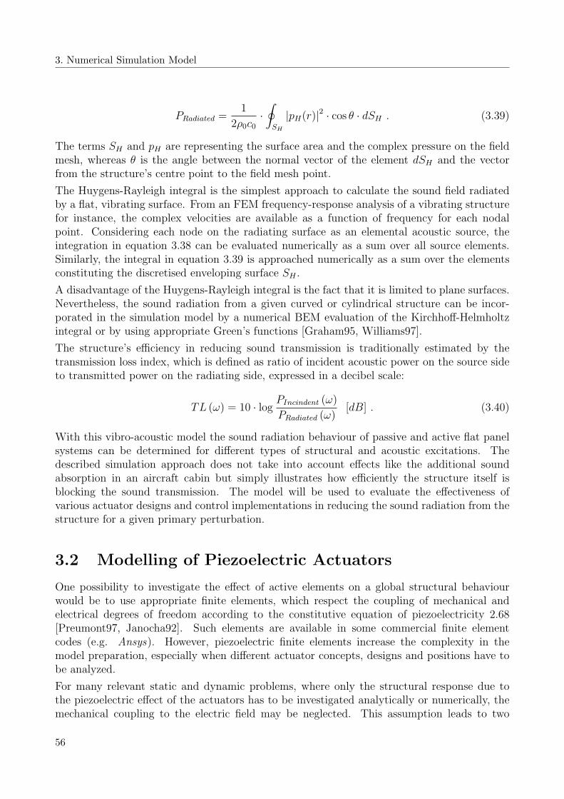
3. Numerical Simulation Model
PRadiated =1
2ρ0c0·∮
SH
|pH(r)|2 · cos θ · dSH . (3.39)
The terms SH and pH are representing the surface area and the complex pressure on the fieldmesh, whereas θ is the angle between the normal vector of the element dSH and the vectorfrom the structure’s centre point to the field mesh point.
The Huygens-Rayleigh integral is the simplest approach to calculate the sound field radiatedby a flat, vibrating surface. From an FEM frequency-response analysis of a vibrating structurefor instance, the complex velocities are available as a function of frequency for each nodalpoint. Considering each node on the radiating surface as an elemental acoustic source, theintegration in equation 3.38 can be evaluated numerically as a sum over all source elements.Similarly, the integral in equation 3.39 is approached numerically as a sum over the elementsconstituting the discretised enveloping surface SH .
A disadvantage of the Huygens-Rayleigh integral is the fact that it is limited to plane surfaces.Nevertheless, the sound radiation from a given curved or cylindrical structure can be incor-porated in the simulation model by a numerical BEM evaluation of the Kirchhoff-Helmholtzintegral or by using appropriate Green’s functions [Graham95, Williams97].
The structure’s efficiency in reducing sound transmission is traditionally estimated by thetransmission loss index, which is defined as ratio of incident acoustic power on the source sideto transmitted power on the radiating side, expressed in a decibel scale:
TL (ω) = 10 · logPIncindent (ω)
PRadiated (ω)[dB] . (3.40)
With this vibro-acoustic model the sound radiation behaviour of passive and active flat panelsystems can be determined for different types of structural and acoustic excitations. Thedescribed simulation approach does not take into account effects like the additional soundabsorption in an aircraft cabin but simply illustrates how efficiently the structure itself isblocking the sound transmission. The model will be used to evaluate the effectiveness ofvarious actuator designs and control implementations in reducing the sound radiation from thestructure for a given primary perturbation.
3.2 Modelling of Piezoelectric Actuators
One possibility to investigate the effect of active elements on a global structural behaviourwould be to use appropriate finite elements, which respect the coupling of mechanical andelectrical degrees of freedom according to the constitutive equation of piezoelectricity 2.68[Preumont97, Janocha92]. Such elements are available in some commercial finite elementcodes (e.g. Ansys). However, piezoelectric finite elements increase the complexity in themodel preparation, especially when different actuator concepts, designs and positions have tobe analyzed.
For many relevant static and dynamic problems, where only the structural response due tothe piezoelectric effect of the actuators has to be investigated analytically or numerically, themechanical coupling to the electric field may be neglected. This assumption leads to two
56

3.2 Modelling of Piezoelectric Actuators
relative simple models, where the additional strain induced by the actuators is replaced withan equivalent thermal load or a set of external, static forces applied along the edges of thepiezo-element.
To derive a suitable actuator concept for the control of sound transmission through an aircraftsidewall section, both models will be used in the simulations presented in Chapter 4. Themechanical principles and assumptions underlying those models are shortly summarized in thefollowing sections.
Thermal-Elastic Analogy
The thermal-elastic analogy is based on the mathematical similarity between free piezoelectricand thermal strain to model the piezoelectric effect. If the governing equation 2.66 for apiezoceramic material polarized in 3-direction is expanded to include thermal strain effects,the following system of equations describing the in-plane behaviour of the material is obtained:
σ1
σ2
τ12
=
Q11 Q12 0Q12 Q22 00 0 Q66
·
·
ǫ1ǫ2γ12
−
0 0 d31
0 0 d31
0 d15 0
·
U1/t1U2/t2U3/t3
−
αα0
· ∆T
, (3.41)
which can be expressed in matrix notation as:
⇔ (σ) = [Q] ·(ǫ− Λ − α · ∆T
). (3.42)
The term Q denotes the stiffness matrix relating the strain to the stress state of the material.As can be seen from equation 3.41, the in-plane response due to an electric field in 3-direction issimilar to the thermal strain induced by the temperature load ∆T . Consequently the actuatorexcitation d31 · U3/t3 can be modelled by replacing the free piezoelectric strain Λ with anequivalent thermal strain α · ∆T applied to the piezoelectric material [Rapp96]. The rest ofthe structure is assumed to have a thermal expansion coefficient equal to zero. This method iseasy to use because most FEM-programs can take into account thermal strain effects and givesacceptable results when the influence of active elements on global structural displacements isexamined.
To numerically validate the FEM-model of Thunder elements, a set of actuators (modelTH-10R, shown on the left side of Figure 2.13) was purchased for testing. The basic propertiesof this actuator type, provided by the manufacturer, are listed in Table 3.1.
A simplified structural model of this actuator element was built up in Nastran using CQUAD4elements for the substrate steel layer and CHEXA volume elements for the ceramic layer. Thecurvature of the element is not considered in the model, as it is very small in comparisonto the length and width of the element. The adhesive layers and the mounting slots on thefree tabs are neglected as well within the FEM-model. The piezoelectric effect is modelledwith the thermal-elastic analogy. The material properties and various parameters used in the
57

3. Numerical Simulation Model
Table 3.1: Thunder specifications for model TH-10R
Thunder Specifications
Overall dimensions: 25,4 x 13,8 x 0,64 mm
PZT-dimensions: 12,7 x 12,7 mm
Composite thickness: 0,43 mm
Substrate layer thickness: 0,20 mm
PZT layer thickness: 0,20 mm
Weight: 0,8 g
Capacity: 9 nF
Max. voltage (Vpp): 480 V
Typical displacement∗: 0,3 mm
Blocked force∗∗: 36 N
∗ clamped support on one side, maximum input voltage,quasi-static deflection peak to peak of the free tip at 1 Hz∗∗ simply supported
FEM-model are summarized in Table 3.2. When the element is clamped in a cantileveredbeam configuration a sinusoidal voltage, or a temperature load respectively, applied to theceramic layer, induces a bending moment in the element and the free tip will make an up- anddownward deflection as shown in Figure 3.5 for a harmonic excitation with 450 Hz.
Table 3.2: Thunder FEM-properties
Substrate Layer Ceramic Layer
Material: steel PZT-5A
Y.-modulus: 210.000 N/mm2 60.600 N/mm2
Poisson-constant: 0,3 0,3
Density: 7,85 g/cm3 7,80 g/cm3
Dimensions: 0,2 mm thickness 0,2 mm thickness
25,4 x 13,8 mm 12,7 x 12,7 mm
Mesh: CQUAD4 elements CHEXA elements
Boundary condition: cantilevered mount nil
Thermal exp. coefficient: 0 K−1 6, 3 · 10−5 K−1
Damping: modal damping of 1% modal damping of 1%
On the real Thunder element this deflection of the free tip was measured with a laser vibrom-eter. The curves in Figure 3.6 show four frequency-response functions in terms of normalvelocity per applied voltage obtained with frequency sweeps from 0 to 1 kHz. The experimen-tal results differ in magnitude and frequency because the cantilever mounting of the elementswas repeatedly dis- and reassembled for the measurements. The velocity magnitude reachesits maximum between 400 and 500 Hz when the first bending eigenmode of the element is fullyexcited.
58

3.2 Modelling of Piezoelectric Actuators
Figure 3.5: FEM-model: structural deflection, driving frequency 450 Hz
0 100 200 300 400 500 600 700 800 900 10000
0.002
0.004
0
0.006
0.008
0.01
0.012
Vel
ocity
/ V
olta
ge [m
/Vs]
Velocity Magnitude
0 100 200 300 400 500 600 700 800 900 10000
0.002
0.004
0.006
0.008
0
0.01
0.012
Vel
ocity
/ ∆
Tem
pera
tur
[m/K
s]
Frequency [Hz]
FEM−simulation
0 100 200 300 400 500 600 700 800 900 1000−300
−200
−100
0
100
200
Pha
se [°
]
Velocity Phase
Frequency [Hz]0 100 200 300 400 500 600 700 800 900 1000
−300
−200
−100
0
100
200
Pha
se [°
]
Experiment
Figure 3.6: Measured and calculated actuator frequency-response
Based on the experimental data, the thermal expansion coefficient of the ceramic layer in theFEM-model was then calibrated in such a way that the velocity response of the numericalmodel per one degree Kelvin matches the experimental velocity response per one Volt, usingthe same geometrical and boundary conditions as in the experiment. The simulation resultsin Figure 3.6 show that a good agreement in magnitude and phase for both numerical andmeasured data is reached. The thermal expansion coefficient utilised in the thermal-elasticmodel is equal to 6, 3 · 10−5 K−1.
Equivalent Force Model
Another method is provided by the equivalent force model in which the actuator stiffness andactuation forces are replaced by a set of equivalent line forces and moments applied to therespective FEM-nodes of the host structure along the edges of the particular piezo patch. Theequivalent forces and moments correspond to the stress resultants, which are obtained from the
59
3. Numerical Simulation Model
equilibrium of forces for a small structural element as illustrated in Figure 3.7 for a structurewith a surface bonded piezo patch.
Reference
Plane
z
NyMyx
NyxMy
MxNxy
NxMxy
Piezo Patch
Laminate
Plate
z
x y
t
Figure 3.7: Laminate plate with a surface bonded piezo patch
For plates made of orthotropic laminate layers the equivalent force model can be derived withthe classical laminate theory [Locatelli01]. The resulting equivalent in-plane forces are givenby the following equation in matrix form:
(NM
)
eq
=
[A BB D
]
hs
·[A BB D
]−1
tot
·[AB
]
act
· Λ , (3.43)
where N = Nx, Ny, NxyT and M = Mx,My,MxyT . A, B and D are the usual stiffnessmatrices as used in the classical laminate theory [Rohwer96, Tsai80]. Its ij-th elements aredefined as:
Matrix of in-plane stiffness: Aij =N∑
k=1
Qij,k · (zk − zk−1) ,
Matrix of coupling stiffness: Bij =1
2·
N∑
k=1
Qij,k ·(z2
k − z2k−1
),
Matrix of rotational stiffness: Dij =1
3·
N∑
k=1
Qij,k ·(z3
k − z3k−1
), (3.44)
with Qij,k being the ij-th element of the reduced stiffness matrix Q in the k-th laminate layerand zk the coordinate through the laminate thickness t. The subscripts hs, tot and act refer tothe summation over the host structure only, the whole structure including the actuators andthe actuators only, respectively. Although equation 3.43 is only valid for static applications,it has been shown that with the equivalent force model proper results are also obtained fordynamic problems [Bebesel99, Lammering98, Locatelli01, Nijhuis03]. However, as in contrastto the thermal-elastic model the influence of actuator mass and stiffness are neglected indynamic analysis, the dynamic application is limited to piezo patches with small dimensions in
60

3.3 Control Loop Simulation
comparison to the host structure. Furthermore, for a given material combination of structureand piezoceramic, relation 3.43 can be used to optimise the actuator thickness with respect tothe actuation forces. A more detailed description and derivation of the equivalent force modelis covered in the Annex A.
3.3 Control Loop Simulation
For the simulation of the control loop, the structural behaviour is described by the followingset of second order differential equations:
Ms · X(t) + Cs · X(t) +Ks ·X(t) = Rs(t) = Rp(t) +Ra(t) , (3.45)
Ra(t) = −Pa · Ua(t) = −Pa ·H · Ys(t) . (3.46)
The vector Rs is the load vector and is composed of a primary perturbation Rp and a secondarycontroller generated part Ra defined in equation 3.46. The matrix Pa relates the structuralload to the actuator input signal Ua, which in turn might be expressed as product of a generalcontroller matrix H and an output signal Ys used as error quantity. Depending on the controlalgorithm and sensor types either appropriate structural velocities:
Ys(t) = C1 · X(t) , (3.47)
or accelerations output signals:
Ys(t) = C1 · X(t) , (3.48)
are available. The influence matrix C1 relates the sensor distribution to the velocity or accel-eration vector.
A second output Yr is required to monitor the velocities on the radiating surfaces, which arethen post-processed to calculate the radiated sound power as described in Chapter 3.1.3. Theyare related to the velocity vector X by a second influence matrix C2:
Yr(t) = C2 · X(t) . (3.49)
Many controller design methods are based on the state space description of the system tobe controlled. With this model any linear, time-invariant, dynamical system as given bythe equations 3.45 to 3.49 can be described with a set of first order differential equations[Preumont97]:
X(t) = A ·X(t) +B · U(t) , (3.50)
Y (t) = C ·X(t) +D · U(t) . (3.51)
The first equation describes the internal dynamics of the system, represented by the statevector X, when driven by the input vector U . The matrix A is the system matrix and B the
61

3. Numerical Simulation Model
input matrix. The system output is given by equation 3.51 and relates the output vector Y tothe state and input vector by the output matrix C and the feedthrough matrixD, respectively3.
To simplify the simulation model only the steady state response to a tonal primary perturbationis considered. With this presumption, the calculation of the structural dynamics withoutcontrol and the closed-loop behaviour can both be performed in the frequency domain and amore complex description in the time domain is not necessary. The frequency domain formof the state space model is obtained by a Laplace transformation of equations 3.50 and 3.51.Thus, the state equation becomes (assuming zero initial conditions):
X(s) = (sI − A)−1 ·B · U(s) , (3.52)
and from the output equation 3.51 the relation:
Y (s) =[C · (sI − A)−1 ·B +D
]· U(s) = G(s) · U(s) , (3.53)
is obtained. For a MIMO system G(s) is the transfer matrix consisting of N × M linear,time-invariant transfer elements G(s) = [yi(s)/uj(s)] (i = 1, 2, . . . , N ; j = 1,2,. . . ,M), with Mbeing the number of input signals and N the number of output signals.
X YsC1
C2
StructureRp U
Ra
PaUa
H
Yr
-
Actuator Controller
Sound Radiation
Error SensorsPrimary
Perturbation
Figure 3.8: Control Loop
The block diagram of a typical control loop, representing the simulation model described byequations 3.45 to 3.49, is illustrated in Figure 3.8. It is assumed that the structure, possessingM independent degrees of freedom, is fitted with Ns sensors and Na actuators. Additionallythe sound radiation is monitored at Nr local points. According to equation 3.53 the inputvector U and output vector Ys, which is used as error signal for the control, are related bya transfer matrix G1 ∈ C
Ns×M . In an analogous manner a transfer matrix G2 ∈ CNr×M
connects the input to the second output signal Yr. A generic control law is represented bythe block containing the transfer matrix H ∈ C
Na×Ns . It generates the actuator driving signalUa, which is linked to the actuator load Ra and the input vector U by the influence matrixPa ∈ C
M×Na . If an appropriate control law is used, the effect of the primary perturbation Rp
on the output signal Ys can be compensated to a great extent. For the present application,two control algorithms, namely local velocity feedback and LMS control, are implemented inthe simulation model.
3Note that the state vector X should not be confounded with the displacement vector X.
62

3.3 Control Loop Simulation
However, as the error signal Ys and output signal Yr, from which the radiated sound field isderived, do normally not correspond and given that the purpose of control is to reduce thestructural sound radiation, error sensors having a good as possible correlation to the radiatedsound are required. Since the square velocity of a radiating element is proportional to theradiated sound power (see equation 3.39), suitable error signals are for instance local structuralvelocities or accelerations as given by equations 3.47 or 3.48.
Local Velocity Feedback
Local velocity feedback control is often mentioned in literature about active structural control[Hansen97, Locatelli01, Nijhuis03] and is based on the negative feedback of a velocity sensorsignal to a given actuator through a proportional gain. Because the control forces appear asviscous damping terms in the equations of motion and increase the dissipation of power, thecontrol law is often referred to as active damping. Using collocated actuators and sensorsensures the stability of the system for a given gain range and provides a certain robustnessto uncertainties in the structural model [Preumont97]. The complexity of a hardware systemusing velocity feedback control is rather low because only analogue elements would be requiredfor its implementation.
The control law can be derived from the scheme in Figure 3.8. The error signal consists of theperturbation signal and the secondary signal:
Ys(s) = G1 · U(s) = G1 · (Rp(s) − Pa · Ua(s)) . (3.54)
Replacing Ys(s) by the following relation:
Ua(s) = H · Ys(s) , (3.55)
the driving signal Ua(s) is obtained as function of the primary perturbation signal:
Ua(s) = (I +HG1Pa)−1 ·H ·G1 ·Rp(s) . (3.56)
Each collocated actuator and sensor pair represents a single-input single-output system. Hence,the gain matrixH is reduced to a diagonal matrix of the formH = diag(hi) with i = 1, 2, . . . , Ns
and Ns = Na.
Least-mean-square control
Another control law, which might be used for the control of tonal or stochastic perturbationsas in the present application, is the LMS algorithm [Hansen97, Maier00, Maier02, Nijhuis03].The hardware implementation is more complex than for the velocity feedback algorithm andrequires digital signal processing with adaptive filters [Elliott01a, Widrow85]. More detailsabout the experimental implementation are given in Chapter 5. The objective of the controlalgorithm is the minimization of a cost function J . As physical quantity a mean, quadraticvibration level being proportional to the transmitted sound power is often used:
J(s) = Y Hs (s) · Ys(s) →Min . (3.57)
63

3. Numerical Simulation Model
In this case Ys is the acceleration output signal as defined by equation 3.48. Taking intoaccount equation 3.54, the cost function J is a quadratic function with respect to the actuatorsignal Ua and thus has distinct minima, which can be determined by setting the derivative ofJ by Ua to zero. The derivative of J with respect to Ua is expressed as:
∂J
∂Ua
= −2 · (G1Pa)H ·G1 · (Rp(s) − Pa · Ua(s)) = −2 · (G1Pa)
H · Ys(s) = 0 . (3.58)
Solving for the actuator command Ua(s) results in:
Ua(s) =((G1Pa)
H ·G1Pa
)−1 · (G1Pa)
H ·G1 ·Rp(s) . (3.59)
The superscript H denotes the Hermitian matrix. In terms of error signal reduction, theactuator input signal Ua(s) defined by equation 3.59 represents the optimal solution. Therefore,the simulated system with LMS control corresponds to an optimal adaptive feed-forward controlconcept without causality constraints.
Sound Radiation
As the error signals and the database needed to calculate the radiated sound field do normallynot coincide, the controlled structural response has to be calculated in an analogous manneras described above using the superposition principle. With a known actuator command Ua(s)the output signal Yr(s) on the vibrating surface becomes:
Yr(s) = G2 · U(s) = G2 · (Rp(s) − Pa · Ua(s)) . (3.60)
The term G2 ·Rp(s) contains the velocities on the radiating structural parts due to the primaryperturbation and the expression G2 · Pa · Ua(s) describes the velocities due to the actuatorexcitation. With Yr as input, the sound radiation is evaluated by the Huygens-Rayleigh integralfor the open and closed-loop system.
The computation of the actuator transfer matrices Gi ·Pa and the primary perturbation vectorGi · Rp, with i = 1, 2, is done in Nastran, whereas Matlab is used to calculate the actuatorinput signal Ua, the resulting output Yr and the radiated sound power.
For broadband primary noise it is much more difficult to obtain a realistic performance pre-diction of the closed-loop behaviour. Nevertheless, in this case the frequency domain approachmay be used as a simple performance estimate of ANVC systems if causality constraints areneglected [Elliott01a].
3.4 Validation of the Simulation Procedure
An experimental validation of the numerical transmission loss prediction tool is presented inthis chapter. The test setup is consisting of a single aluminium panel, a double wall configu-ration consisting of two identical aluminium panels and a double wall configuration, where theabsorption in the cavity is enhanced with a thin layer of porous absorption material. The model
64
3.4 Validation of the Simulation Procedure
is validated by comparing the predicted and measured relative sound power levels radiated bythe structure for various excitations.
The measurements are carried out with aluminium panels having in-plane dimensions of 1 by1 m and a thickness of 1 mm. A separation distance of 90 mm between the single panels ischosen for the double wall configuration. To determine the sound transmission behaviour thepanels are clamped with a set of frames in a transmission loss test window situated betweena reverberation and anechoic chamber. The reverberation room is used for the excitation onthe incident side of the panel, which is either done with a diffuse sound field through a pair ofloudspeakers or a point force driving directly the panel. Both excitation sources are driven bya white noise source. In the anechoic chamber the transmitted sound power is measured byscanning the sound intensity over the surface of the radiating structure with an appropriatemicrophone system. The incident sound power is obtained from the diffuse sound pressure levelin the reverberation chamber [Heckl94]. According to equation 3.40 and the European StandardNorm EN ISO 15186-14, the transmission loss is derived as ratio of incident to transmittedsound power. For the point force excitation the transmitted sound power is related to theexcitation force. The measurement setup and method are described in detail in Chapter 5.2.
In Nastran each panel is modelled by 1224 uniform CQUAD4 shell elements and is clamped onits edges in an infinite, rigid baffle preventing both rotational and translatory displacements.For the double wall configurations the cavity fluid is modelled with 3756 CHEXA solid elementsmatching the structural mesh of the aluminium panel. On the wetted surface of the structurethe dynamical behaviour of the structural and fluid domain is coupled through the normalcomponents of velocity, whereas on all surfaces of the fluid not in contact with the structure,a boundary condition of vn = 0 is enforced. The dynamic response of the radiating panel isdetermined by a modal frequency-response analysis. As the acoustical behaviour of the setupis determined in a frequency range up to 500 Hz, eigenmodes up to 1 kHz are retained inthe summation of the modal responses [Blakely93]. Thus, the solution space is based on 298eigenmodes for a single aluminium panel and 32 eigenmodes for the cavity fluid. A step sizeof 2,5 Hz is selected for the frequency resolution. Material and FEM-parameters for this basicconfiguration, denoted as configuration one in the following, are summarised in Table 3.3.
The main parameters controlling the sound radiation in the simulation model are the structuralenergy dissipation governed by the modal damping parameters, the type of boundary conditionapplied to the structure and the energy dissipation in the cavity fluid. To demonstrate theinfluence of those variables two further configurations in addition to the one resumed in thetable above are analysed numerically. In a second configuration the modal damping applied tothe structure is increased to 3%, whereas for the third configuration the clamped panel supportis replaced with a simply supported boundary condition. The influence of cavity absorptionis considered with a further FEM-model, where the cavity fluid is partly covered by acousticabsorber elements.
Three different types of excitation are used in the numerical simulation. The first modelconsists of a single monopole source located at x = −5 m, y = −1, 5 m and z = 5 m relative tothe panel’s centre point, x and y being the axes in the panel plane and z the normal axis to thepanel. For a typical single aisle aircraft this source position relative to the structure correspondsto the position of the engine inlet relative to the forward fuselage and thus can be regarded as
4Measurement of sound insulation in buildings and of building elements using sound intensity
65

3. Numerical Simulation Model
Table 3.3: Basic experimental and simulation configuration
Aluminium Panel
Y.-modulus: 74.000 N/mm2
Poisson-constant: 0,3
Density: 2,70 g/cm3
Dimensions: 1,0 mm thickness
1000 x 1000 mm
90 mm double wall distance
Mesh: 36 x 36 CQUAD4 elements
Boundary condition: clamped in infinite, rigid baffle
Damping: modal damping of 1%
Fluid
Density: 1,225 kg/m3
Speed of sound: 340 m/s
Spatial decay rate: 0,0001 m−1
(equals a loss factor η of 5, 5 · 10−5)
Mesh: 2 x 34 x 34 CHEXA elements
1 x 38 x 38 CHEXA elements
Boundary condition: structural velocity or vn = 0
a simple approximation for a buzz-saw noise excitation. The resulting incidence angle on thepanel is about 46, which for a typical buzz-saw noise directivity pattern corresponds to thedirection with maximal intensity [Lewy00].
A diffuse excitation is modelled by plane wave superposition. According to the field incidencemass law an approximated diffuse sound field is constructed from 250 independent monopolesources with incidence angles ranging from 0 to 78 to equal all relevant directions of incidence.Their position is distributed randomly over a half sphere of radius r = 100 m, covering thestructure’s incident side. Each monopole is given a constant source strength and a randomfrequency-dependant phase αn. The point force excitation is modelled with a normal unityload of 1 N placed at the same relative position as in the experiments (x = 222 mm andy = 280 mm relative to the panel’s centre point).
To derive the structurally radiated sound power in the numerical model, the Rayleigh integralis evaluated on a half cube of 100 m length, which totally covers the radiating structure.The cube is discretised into a relatively coarse field point mesh consisting of 108 uniform,rectangular elements where the resulting sound pressure is analysed. The accuracy of theRayleigh approach was checked by calculating the sound radiation from a 2 mm steel panelexcited by a point force and comparing the results with those obtained from a direct BEM-analysis in LMS/Sysnoise. The sound power predicted by both methods was in good agreement.The mean error averaged from 0 to 500 Hz amounted 1,4% or 0,06 dB, whereas the maximumerror was 6,2%, corresponding to a difference of 0,3 dB in radiated sound power level. However,the main benefit from using the Rayleigh integral in combination with the far field assumptionis the fact that the computation time needed to process the sound power from the structural
66

3.4 Validation of the Simulation Procedure
vibration data is at least reduced by 95% in comparison to the BEM-method.
It should be mentioned that an absolute comparison of measured and predicted sound trans-mission behaviour is only possible to some extent, as due to the respective measurement setup(geometry of the test window, mounting condition of the test structure, acoustic characteristicsof test chambers) measured transmission loss values may vary up to 5 dB in the consideredfrequency range. Detailed analysis of those effects can be found in numerous publications[Guy84, Halliwell85, Jones79, Kihlman72, Kim04, Warnock82].
Aluminium Single Wall Partition
The predicted and measured transmission loss curves for the single panel with monopole anddiffuse excitation are illustrated in Figure 3.9 and 3.10. In both cases there is a reasonableagreement between the predicted and measured sound transmission behaviour. In Figure 3.9the dashed curve represents the mass law for 45 incidence, whereas in Figure 3.10 the dashedcurve is calculated from the field incidence mass law. The results obtained with the point forceexcitation are represented in Figure 3.11 by means of radiated sound power relative to thesquare excitation force.
0 50 100 150 200 250 300 350 400 450 500−5
0
5
10
15
20
25Transmission Loss
Frequency [Hz]
TL
[dB
]
R(45°) Exp. Sim. Config. 1Sim. Config. 2Sim. Config. 3
Figure 3.9: Transmission loss with monopole excitation
In the low-frequency range single eigenmodes with high radiation efficiency are excited on thereal structure and in the simulation models, resulting in transmission loss values well belowthe one given by the analytical models. In-between those modes other eigenmodes with lowsound radiation efficiency and a high transmission loss can be found. For higher frequenciesthe modal density is increased and the calculated and measured transmission loss curves are
67

3. Numerical Simulation Model
0 50 100 150 200 250 300 350 400 450 500−5
0
5
10
15
20
25Transmission Loss
Frequency [Hz]
TL
[dB
]
R(0°) − 5 dB Exp. Sim. Config. 1Sim. Config. 2Sim. Config. 3
Figure 3.10: Transmission loss with diffuse excitation
0 50 100 150 200 250 300 350 400 450 500−60
−55
−50
−45
−40
−35
−30
−25
−20
−15Sound Power per Square Force
Frequency [Hz]
Sou
nd P
ower
[dB
(1 m
/N/s
)]
Exp.Sim. Config. 1Sim. Config. 2Sim. Config. 3
Figure 3.11: Sound power per square excitation force
68

3.4 Validation of the Simulation Procedure
smoothed and converge towards the theoretical mass laws showing the well-known behaviourof 6 dB increase per doubling of frequency.
The effect of mass control on the sound transmission, also connected with an increase of 6 dBper doubling of mass, is reproduced as well with the simulation approach, but not furthershown here. In comparison to the monopole excitation the diffuse sound field results in atransmission loss behaviour exhibiting statistical fluctuations from the mean transmission loss.This is due to the random character of the incident sound field and is also observed in themeasurement data.
The influence of the structural energy dissipation on the sound radiation is obvious fromcomparing the respective simulation results of configuration 1 to configuration 2. By increasingthe modal damping up to 3% the resonant components in the sound transmission are reduced.Therefore, the distinct minima in transmission loss are increased and maxima decreased. Themean transmission loss, governed by the non-resonant mass law, is not affected.
The impact of the structural boundary condition is reflected by the curves representing con-figuration 3. As consequence of replacing the clamped support with a simply supported one,the shape of eigenmodes forming the solution space is changed and eigenfrequencies are shiftedtowards lower frequencies. Hence, the minima and maxima in transmission loss behaviour arealso altered towards lower frequencies. However, as at higher frequencies the influence of theresonant transmission path is reduced, the sound transmission is mainly controlled by the masslaw resulting in a similar mean transmission loss as achieved with the clamped support.
Aluminium Double Wall Partition
The results for the double wall configuration are shown in Figure 3.12 for the acoustic excitationand in Figure 3.13 for the point force excitation. The 45 incidence mass law for double wallpartitions (see equation 2.47), predicting a local minimum in transmission loss at 246 Hz dueto the mass-air-mass resonance5, is illustrated by the dashed curve.
Compared to the analytical model the measured and calculated sound transmission behaviouris far more complex, but as before, especially in consideration of the complexity of the coupledsystem, a good agreement between measured and calculated trends can be observed. Thepredicted sound transmission shows the same characteristics as the measured transmissionloss. A number of resonance frequencies, where the behaviour of both panels is coupled verystrongly through the fluid domain, can be found in the whole frequency range. At thosepoints the transmission loss value is well below the value of a single wall partition basedupon the same total mass as used for the double wall system. Between the minima values,frequencies corresponding to acoustic anti-resonances of the cavity can be found and the motionof both plates is decoupled resulting in high transmission loss values. It should be noted thatthe accordance of the predicted peak at 167 and 242 Hz with the analytical mass-air-massresonance is incidental. In contrast to the mass law, which is only valid for infinite panels, thecomplex coupling between structural and fluid eigenmodes in the numerical model is stronglydependant on additional parameters like the absolute dimensions of the structure and the fluidcavity and its boundary conditions.
5The fundamental mass-air-mass resonance occurs at 172 HZ for normal incidence.
69

3. Numerical Simulation Model
0 50 100 150 200 250 300 350 400 450 500−15
−10
−5
0
5
10
15
20
25
30
35
40Transmission Loss
Frequency [Hz]
TL
[dB
]
R(45°)Exp.Sim. Config. 1 MonopoleSim. Config. 1 DiffuseSim. Config. 2 MonopoleSim. Config. 2 Diffuse
Figure 3.12: Transmission loss with acoustic excitation
0 50 100 150 200 250 300 350 400 450 500−60
−55
−50
−45
−40
−35
−30
−25
−20
−15Sound Power per Square Force
Frequency [Hz]
Sou
nd P
ower
[dB
(1 m
/N/s
)]
Exp. Sim. Config. 1Sim. Config. 2
Figure 3.13: Sound power per square excitation force
70
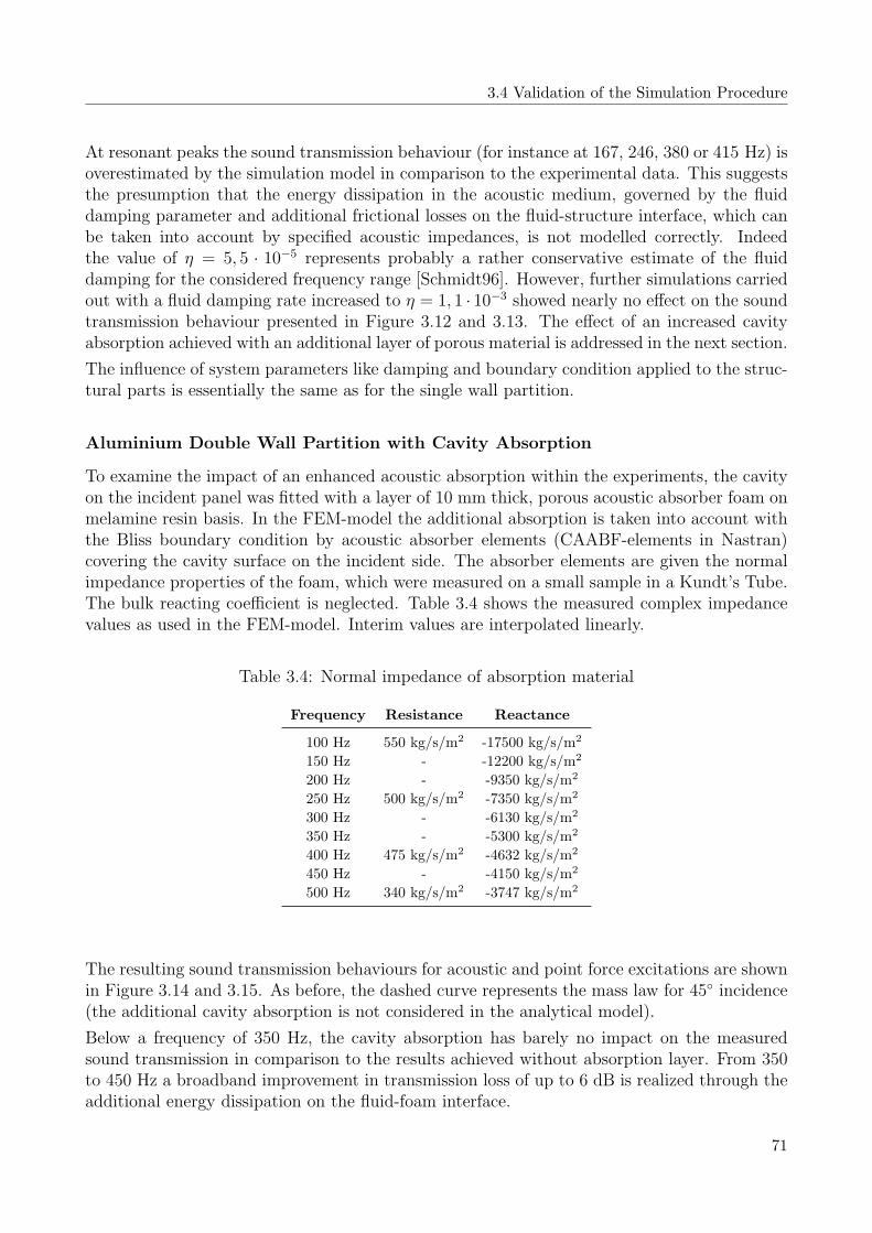
3.4 Validation of the Simulation Procedure
At resonant peaks the sound transmission behaviour (for instance at 167, 246, 380 or 415 Hz) isoverestimated by the simulation model in comparison to the experimental data. This suggeststhe presumption that the energy dissipation in the acoustic medium, governed by the fluiddamping parameter and additional frictional losses on the fluid-structure interface, which canbe taken into account by specified acoustic impedances, is not modelled correctly. Indeedthe value of η = 5, 5 · 10−5 represents probably a rather conservative estimate of the fluiddamping for the considered frequency range [Schmidt96]. However, further simulations carriedout with a fluid damping rate increased to η = 1, 1 · 10−3 showed nearly no effect on the soundtransmission behaviour presented in Figure 3.12 and 3.13. The effect of an increased cavityabsorption achieved with an additional layer of porous material is addressed in the next section.
The influence of system parameters like damping and boundary condition applied to the struc-tural parts is essentially the same as for the single wall partition.
Aluminium Double Wall Partition with Cavity Absorption
To examine the impact of an enhanced acoustic absorption within the experiments, the cavityon the incident panel was fitted with a layer of 10 mm thick, porous acoustic absorber foam onmelamine resin basis. In the FEM-model the additional absorption is taken into account withthe Bliss boundary condition by acoustic absorber elements (CAABF-elements in Nastran)covering the cavity surface on the incident side. The absorber elements are given the normalimpedance properties of the foam, which were measured on a small sample in a Kundt’s Tube.The bulk reacting coefficient is neglected. Table 3.4 shows the measured complex impedancevalues as used in the FEM-model. Interim values are interpolated linearly.
Table 3.4: Normal impedance of absorption material
Frequency Resistance Reactance
100 Hz 550 kg/s/m2 -17500 kg/s/m2
150 Hz - -12200 kg/s/m2
200 Hz - -9350 kg/s/m2
250 Hz 500 kg/s/m2 -7350 kg/s/m2
300 Hz - -6130 kg/s/m2
350 Hz - -5300 kg/s/m2
400 Hz 475 kg/s/m2 -4632 kg/s/m2
450 Hz - -4150 kg/s/m2
500 Hz 340 kg/s/m2 -3747 kg/s/m2
The resulting sound transmission behaviours for acoustic and point force excitations are shownin Figure 3.14 and 3.15. As before, the dashed curve represents the mass law for 45 incidence(the additional cavity absorption is not considered in the analytical model).
Below a frequency of 350 Hz, the cavity absorption has barely no impact on the measuredsound transmission in comparison to the results achieved without absorption layer. From 350to 450 Hz a broadband improvement in transmission loss of up to 6 dB is realized through theadditional energy dissipation on the fluid-foam interface.
71

3. Numerical Simulation Model
0 50 100 150 200 250 300 350 400 450 500−15
−10
−5
0
5
10
15
20
25
30
35
40Transmission Loss
Frequency [Hz]
TL
[dB
]
R(45°)Exp.Sim. Config. 1 MonopoleSim. Config. 1 DiffuseSim. Config. 2 MonopoleSim. Config. 2 Diffuse
Figure 3.14: Transmission loss with acoustic excitation
0 50 100 150 200 250 300 350 400 450 500−60
−55
−50
−45
−40
−35
−30
−25
−20
−15Sound Power per Square Force
Frequency [Hz]
Sou
nd P
ower
[dB
(1 m
/N/s
)]
Exp.Sim. Config. 1Sim. Config. 2
Figure 3.15: Sound power per square excitation force
72

3.5 Conclusions
This behaviour is also reflected in the numerical results. Especially in the frequency range fromaround 330 to 450 Hz the transmission loss is increased with maximum improvements reachingaround 9 dB on the local minima at 380 and 415 Hz. This increase is mainly governed by theresistance, whereas due to the reactance the frequencies of coupled fluid-structure modes areshifted towards lower values.
Comparing the measured and predicted sound transmission trends, an acceptable correspon-dence is obtained, even if generally on resonance peaks the sound reduction is still overestimatedby the simulation model.
3.5 Conclusions
A hybrid FEM/Huygens-Rayleigh methodology was presented to predict the sound transmis-sion of plane single and double wall partitions in the low-frequency range. Compared tocommercially available BEM-tools, the method has the advantage of being extremely fast andcan also be used for relatively complex structures [Peiffer05]. Furthermore, based on the su-perposition principle, the influence of a control loop with active elements can be integrated inthe simulation model.
The prediction tool was validated against experimental results obtained from measurementswith various single and double wall configurations. It emerged from the comparison of nu-merical and measured results that an accurate, numerical reproduction of the measured soundtransmission behaviour would be very difficult to realize. This discrepancy is mainly due touncertainties inherent to the model, but also to the experimental results:
• A high complexity is involved with the numerical model, as for instance the solution forthe double wall is based on a total of 628 eigenmodes.
• Some parameters like the structural damping and boundary conditions as well as thefluid damping and frictional losses on the fluid-structure interface are difficult to modelin the considered frequency range, but have a huge impact on the sound transmissionbehaviour.
• It has been shown in literature that a sound transmission loss determined in experimentsdepends very much on the actual measurement configuration and can vary within certainlimits.
However, it should be emphasized that the general sound transmission behaviour is well pre-dicted with the simulation model and in good agreement with measured trends. In the followingchapter the transmission loss prediction tool will be used in the design process of active struc-tural acoustic control systems, intended to increase the transmission loss of aircraft sidewallstructures. For this application the simulation procedure can be considered to be sufficientlyaccurate as the active systems will be only evaluated by their relative performances (soundtransmission behaviour achieved with active control versus open-loop behaviour).
73


Chapter 4
Numerical Study of Active DoubleWall Structures
By means of a simplified, generic double wall structure different actuator and sensor conceptsare evaluated numerically based on the methodology presented in the previous chapter. Theactuation is either done via a number of d31-piezo patches bonded to the fuselage skin or thetrim panel, or with a set of active attachment elements replacing the conventional trim panelattachments. Several sensor concepts can be combined with the actuators in the simulationmodel. With the piezo patches bonded to the fuselage and the trim panel, a local velocityfeedback control law with collocated velocity sensors is used. The intention of such a system isto increase the power dissipation in the structure and to obtain simultaneously a reduction inradiated sound power. In combination with the active attachment elements (hereinafter alsoabbreviated by the term AAE) an LMS control loop with unidirectional acceleration sensorsplaced on the trim panel and the attachment elements is analysed. Furthermore, it is alsopossible to use sound pressure sensors, either located in the fluid cavity or on the radiatingside of the trim panel, as an error signal in combination with the three actuator concepts.
The control concepts are evaluated by their respective performance to increase the transmissionloss of the whole fuselage section, the change of mean acceleration level on the trim panel andthe actuation effort measured by the required actuator voltage. Based on the simulationresults, the most appropriate concept will be realized in a proof-of-concept study and testedexperimentally.
4.1 Structural Model
The FEM-model of the generic, plane fuselage section (the trim panel is shown only to thehalf) and the enclosed cavity is illustrated in Figure 4.1. The fuselage has in-plane dimensionsof 1 by 1 m and consists of a 1,6 mm thick aluminium skin stiffened by six simplified L-shapedstringers and two C-shaped frames. Both stringers and frames are also made of aluminiumand 1,6 mm thick. The height of the frames is 115 mm, whereas the stringers are 29 mmhigh. The spacing between frames and stringers is 500 and 167 mm respectively. On the skinthe stiffening effect of stringer and frame feet is taken into account by strengthening the skinthickness up to 3,2 mm as illustrated by the colored elements in Figure 4.1.

4. Numerical Study of Active Double Wall Structures
Figure 4.1: Structural and fluid FEM-model
The trim panel has the same in-plane dimensions as the fuselage skin and is located 15 mmabove the frames. In the basic configuration it is attached to the fuselage by four rigid barelements1. The structural connections provide a path for structure-borne sound beside theairborne path taken into account by the fluid-structure coupling. The trim panel is modelled asrealistic sandwich structure (ECA-honeycomb core reinforced with phenolic fibreglass prepregskin sheets), representative for typical aircraft interiors.
Both the trim panel and the fuselage skin are clamped on their edges into infinite, rigid baffles.Material and modelling parameters for the fuselage section, the honeycomb core and the skinsheets of the trim panel are specified in Table 4.1.
The fluid between the fuselage and the trim panel is modelled with volume elements matchingthe mesh size of the fuselage and trim panel. Boundary conditions of vn = 0 are enforced onall surfaces of the fluid not in contact with the structure, with vn being the normal velocity onthe fluid surface. To provide an acoustic absorption in the cavity the remaining fluid surface,coupled to the structure, is covered with absorber elements, which are given the same acousticproperties as already used in the previous chapter (see Table 3.4). The FEM-model also takesinto account the fluid interaction with the frames, whereas the interaction with the stringersis neglected. The properties of the fluid model are listed in Table 4.2.
The system response with and without control is simulated in the frequency range from 2,5to 500 Hz. A step size of 2,5 Hz is selected for the frequency resolution. The whole modelhas 37100 degrees of freedom and 208 structural and 37 fluid eigenmodes, forming the modalspace up to 1 kHz, are considered in the frequency response. As primary excitation a coherentmonopole source radiating with an incidence angle of 45 towards the trim panel is used. Infree field conditions the monopole source strength would be equal to a mean sound pressurelevel of 80 dB on the fuselage skin. To analyse the effects of further excitation mechanism anormal unity force acting on the fuselage skin2 and a diffuse sound field similar to the one usedin Chapter 3.4 are considered as well as primary excitation.
1Attachment points: (x = 250 mm; y = 250 mm), (x = 250 mm; y = 750 mm), (x = 750 mm; y = 250 mm)and (x = 750 mm; y = 750 mm), x and y being the in-plane coordinates as shown in Figure 4.1.
2Position: x = 222 mm and y = 280 mm.
76

4.1 Structural Model
Table 4.1: Parameter sidewall structure
Fuselage
Material Aluminium
Y.-modulus: 70.000 N/mm2
Poisson-constant: 0,3
Density: 2,70 g/cm3
Size: 1,6 mm thickness
reinforced to 3,2 mm on frames & stringers
1000 x 1000 x 115 mm
Mesh: Skin 36 x 36 CQUAD4 elements
Stringers 6 x 1 x 36 CQUAD4 elements
Frames 2 x 4 x 36 CQUAD4 elements
Trim Panel, ECA-Honeycomb Core
Material: anisotropic
Shear-modulus: 27 N/mm2 (L-direction)
16 N/mm2 (W-direction)
Poisson-constant: 0,3
Density: 29,0 kg/m3
Size: 5,0 mm thickness
1000 x 1000 mm
Mesh: 36 x 36 CHEXA elements
Trim Panel, Skin Sheets
Material phenolic E-glass prepreg
Y.-modulus: 29.000 N/mm2 (lower skin)
22.000 N/mm2 (upper skin)
Poisson-constant: 0,3
Density: 2,00 g/cm3 (lower skin)
1,82 g/cm3 (upper skin)
Size: 0,20 mm thickness (lower skin)
0,28 mm thickness (upper skin)
1000 x 1000 mm
Mesh: 36 x 36 CQUAD4 elements
General Structural Parameter
Boundary condition: clamped into infinite, rigid baffle
Damping: modal damping of 1%
77

4. Numerical Study of Active Double Wall Structures
Table 4.2: Parameter cavity fluid
Fluid
Density: 1,225 kg/m3
Speed of sound: 340 m/s
Spatial decay rate: 0,0001 m−1 (equals a loss factor of 5, 5 · 10−5)
Mesh: 5 x 36 x 36 CHEXA elements
Boundary condition: vn = 0 on free fluid surfaces
coupled surfaces covered with absorption foam
4.2 Actuator and Sensor Concepts
The efficiency of an active control system is closely linked to the efficiency of the control law,actuators and sensors. To determine the best solution for a double wall fuselage section, threedifferent actuator and sensor concepts in combination with two control laws are numericallyevaluated. From the numerous methods presented in literature (see Chapter 2.4), d31-piezopatches bonded either to the fuselage or the trim panel represent a common, almost classicalcontrol strategy and are selected as two possible alternatives. Using collocated actuators andsensors with a local velocity feedback control loop ensures the stability of such a system andan experimental implementation would require relatively low hardware complexity.
A novel actuator concept is the active attachment element, which dynamically isolates thetrim panel from the fuselage and is able to introduce secondary control signals into the trimpanel. The system requires a different sensor layout and is evaluated with a more complexLMS control loop.
4.2.1 Active Fuselage Skin Damping
The scheme on the left side of Figure 4.2 shows the layout of the d31-piezo patches and sensorson the fuselage structure and their respective denotations. From a practical point of view theactuators can only be placed inside of the fuselage leaving just the bays formed by adjacentstringer and frame pairs as a realistic position. However, a practical implementation of thiscontrol strategy may be difficult to realise as the actuators would be bonded directly to thefuselage skin, which is stressed with every flight cycle due to the cabin pressurisation. Also alarge operational temperature range, roughly from -50 to 110C considering all possible flightconditions, must be taken into account.
The main idea behind this layout is that by controlling the structural vibrations on the incidentpanel the perturbation source strength transmitted across the cavity to the radiating panel isreduced [Carneal93]. In literature this effect is often referred to as active damping because thecontrol reduces the amplitude of the vibrating modes.
In this study each bay of the generic fuselage model is fitted with a 55 by 55 mm d31-piezopatch resulting in a rather complex system with a total of 15 actuators. Therefore, the resultsachieved with this active system will present an upper bound in terms of performance andcomplexity. In the FEM-model the actuators are taken into account by the equivalent force
78
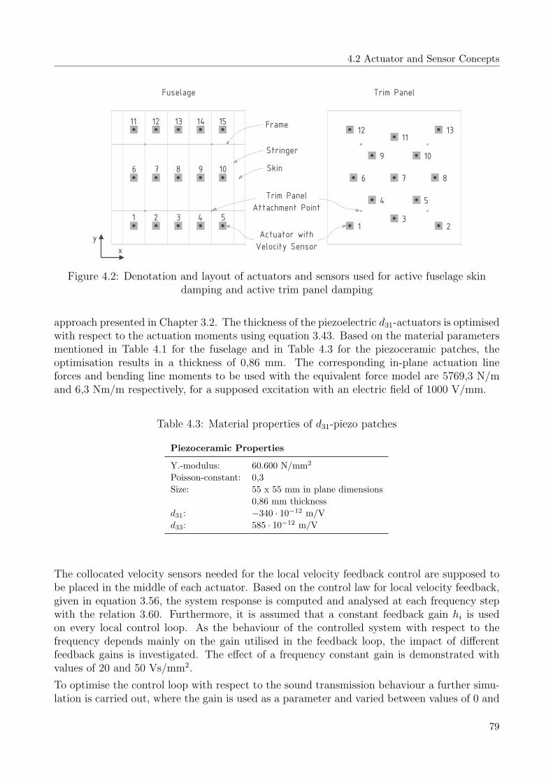
4.2 Actuator and Sensor Concepts
Actuator with
Velocity Sensor
Stringer
Frame
Skin
Trim PanelFuselage
Trim Panel
Attachment Point
y
x
87
9 10
1112 13
1 23
4 5
687 9 10
11 12 13 14 15
1 2 3 4 5
6
Figure 4.2: Denotation and layout of actuators and sensors used for active fuselage skindamping and active trim panel damping
approach presented in Chapter 3.2. The thickness of the piezoelectric d31-actuators is optimisedwith respect to the actuation moments using equation 3.43. Based on the material parametersmentioned in Table 4.1 for the fuselage and in Table 4.3 for the piezoceramic patches, theoptimisation results in a thickness of 0,86 mm. The corresponding in-plane actuation lineforces and bending line moments to be used with the equivalent force model are 5769,3 N/mand 6,3 Nm/m respectively, for a supposed excitation with an electric field of 1000 V/mm.
Table 4.3: Material properties of d31-piezo patches
Piezoceramic Properties
Y.-modulus: 60.600 N/mm2
Poisson-constant: 0,3
Size: 55 x 55 mm in plane dimensions
0,86 mm thickness
d31: −340 · 10−12 m/V
d33: 585 · 10−12 m/V
The collocated velocity sensors needed for the local velocity feedback control are supposed tobe placed in the middle of each actuator. Based on the control law for local velocity feedback,given in equation 3.56, the system response is computed and analysed at each frequency stepwith the relation 3.60. Furthermore, it is assumed that a constant feedback gain hi is usedon every local control loop. As the behaviour of the controlled system with respect to thefrequency depends mainly on the gain utilised in the feedback loop, the impact of differentfeedback gains is investigated. The effect of a frequency constant gain is demonstrated withvalues of 20 and 50 Vs/mm2.
To optimise the control loop with respect to the sound transmission behaviour a further simu-lation is carried out, where the gain is used as a parameter and varied between values of 0 and
79

4. Numerical Study of Active Double Wall Structures
300 Vs/mm2. For each frequency step the values yielding the best transmission loss behaviourare selected. If the resulting transmission loss value obtained with active control should dropbelow the one achieved with open control loop, the control system is consequently turned offfor the respective frequency step. These results will thus present an optimum, which can beattained with a relatively simple local velocity feedback control law.
4.2.2 Active Trim Panel Damping
Another possibility to control the structural response and sound radiation of the trim panel isto use d31-piezo patch actuators, which are placed or directly embedded onto the trim panel. Incontrast to the first solution, this configuration allows a direct control of the radiating surface.Due to a better coherence between the controlled quantities and the sound radiation, the activetrim panel is expected to give better results than the active fuselage skin damping.
The employed actuator layout is shown on the right side of Figure 4.2. Altogether 13 actuatorsare distributed over the trim panel surface. It is assumed that the actuators are placed on theupper skin sheet and as before each active element is fitted with a collocated velocity sensor,which is used for local velocity feedback control.
The thickness optimisation with the equivalent force model results in an optimal actuator thick-ness of 0,96 mm and the line force and moments to be used in the FEM-model are 2243,6 N/mand 1,3 Nm/m. Regarding the sensitivity of the results with respect to the feedback gain, asimilar variation as for the active fuselage skin damping is performed.
4.2.3 Active Attachment Elements
For the evaluation of the concept with active attachment elements the four rigid trim panelattachments are replaced with a set of particular actuators. The sound radiation of the trimpanel is mainly controlled by bending waves [Fahy85, Heckl94] that are excited either by thefluid path through the cavity or by normal translatory and rotational displacement componentsin the plane of the panel and transmitted from the fuselage frames into the trim panel at eachattachment point. Therefore, to control the dynamic behaviour of the trim panel and achievea substantial reduction in sound transmission, it is essential that with each active attachmentelement three degrees of freedom can be controlled independently. To assure the best possibleintegration into the fuselage section, the elements should also have small overall dimensionsand a low weight.
The actuator layout and denotation as well as a prototype CAD-model of an attachmentelement meeting the requirements mentioned above, are illustrated in Figure 4.3. The designis based on Thunder d31-actuators mounted in a clamshell configuration as presented in Chapter2.3.1. In comparison to the Thunder model TH-10R the size of the metal substrate layer isincreased to 32 by 19 mm and the PZT layer to 22 by 19 mm. Otherwise the actuator propertiesas listed in Table 3.1 and 3.2 are retained. The increase of the actuator dimensions is necessarybecause a mounting hole with a diameter of about 4 mm would be required on a real Thunderelement for the force transmission and the attachment of the clamshell units (see also Figure2.15). By using an axis-symmetric layout of three independent clamshell elements arrangedbetween two mounting plates around the attachment points to the trim panel or the fuselageframes respectively, it is possible to excite normal displacements in the z-direction as well as
80

4.2 Actuator and Sensor Concepts
x- and y-rotations between the trim panel and the fuselage. A more detailed illustration of aclamshell actuator unit and an active attachment element is given in Annex B.
Thunder Clamshell
Actuator with
Acceleration Sensor
Stringer
Frame
Skin
Fuselage
Trim Panel
Attachment Point
y
x
AAE 2AAE 1
AAE 3AAE 4
3
7
6
2 5
910
11 8
1 4
12
y
x
z
Active Attachment Element
Position of
Acceleration
Sensor
Thunder
Clamshell
Actuator
Aluminium
Mounting
Plate
Figure 4.3: Denotation and layout of active attachment elements and sensors, CAD-model ofan active attachment element
The hexagonal mounting plates should have a high stiffness to assure the best possible trans-mission of control forces. In the FEM-model they are supposed to be made from aluminium(thickness 3 mm) and their width across the flat side is around 60 mm, whereas the spacingbetween the plates is 10 mm. The radius from the trim panel and fuselage attachment pointsto the attachment of a clamshell unit is 20 mm.
The piezoelectric behaviour of the Thunder elements is modelled by the thermal elastic analogyand a similar structural FEM-model as the one presented in Chapter 2.3.1 is used. The otherstructural parts of the attachment elements are conventionally modelled with shell (mountingplates), solid (clamshell clamping for the Thunder elements) and bar elements (structuralconnections to the mounting plates). By incorporating the active trim panel attachments inthe FEM-model the total number of degrees of freedom is increased to around 130000. Themodal structural base contains a total of 236 modes up to 1 kHz. Fluid interaction with theattachment elements is neglected because for the considered frequency range up to 500 Hzthe maximum dimension of the element is much smaller than the minimum fluid wave length.Otherwise the same simulation parameters as with the other control concepts are used.
Control is performed by the LMS-algorithm with a sensor array of up to 19 unidirectionalaccelerometers. Preliminary investigations with various sensor layouts indicated that for anefficient control of sound radiation different sensor layouts may be required. This is mainly dueto the frequency-dependant dynamic trim panel behaviour and the fact that a single sensorlayout does not give optimal results in terms of sound reduction for the whole frequency range.For this reason the simulation procedure is done for six different sets of sensors containing theinformation of up to 19 unidirectional acceleration sensors placed on the actuators and thetrim panel. By comparing the resulting transmission loss values for every single frequency stepthe best suited sensor concept out of the six is identified.
The six sensor concepts are summarized in Table 4.4. For the first three setups each activeattachment element is fitted with three acceleration sensors placed on the respective upper
81
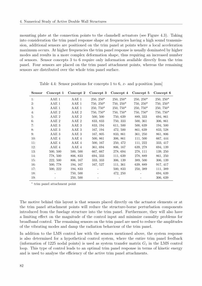
4. Numerical Study of Active Double Wall Structures
mounting plate at the connection points to the clamshell actuators (see Figure 4.3). Takinginto consideration the trim panel response shape at frequencies having a high sound transmis-sion, additional sensors are positioned on the trim panel at points where a local accelerationmaximum occurs. At higher frequencies the trim panel response is usually dominated by highermodes and results in a more complex deformation shape, thus requiring an increased numberof sensors. Sensor concepts 3 to 6 require only information available directly from the trimpanel. Four sensors are placed on the trim panel attachment points, whereas the remainingsensors are distributed over the whole trim panel surface.
Table 4.4: Sensor positions for concepts 1 to 6, x- and y-position [mm]
Sensor Concept 1 Concept 2 Concept 3 Concept 4 Concept 5 Concept 6
1: AAE 1 AAE 1 250, 250* 250, 250* 250, 250* 250, 250*
2: AAE 1 AAE 1 750, 250* 750, 250* 750, 250* 750, 250*
3: AAE 1 AAE 1 250, 750* 250, 750* 250, 750* 250, 750*
4: AAE 2 AAE 2 750, 750* 750, 750* 750, 750* 750, 750*
5: AAE 2 AAE 2 500, 500 750, 639 889, 333 694, 861
6: AAE 2 AAE 2 833, 833 750, 333 500, 361 306, 861
7: AAE 3 AAE 3 833, 194 611, 500 500, 639 194, 500
8: AAE 3 AAE 3 167, 194 472, 500 861, 639 833, 528
9: AAE 3 AAE 3 167, 805 833, 861 361, 250 861, 806
10: AAE 4 AAE 4 500, 861 306, 861 111, 500 667, 444
11: AAE 4 AAE 4 500, 167 250, 472 111, 222 333, 417
12: AAE 4 AAE 4 361, 694 806, 167 639, 278 694, 139
13: 500, 500 500, 500 667, 667 278, 694 278, 111 139, 250
14: 778, 500 806, 833 694, 333 111, 639 278, 889 861, 250
15: 222, 500 806, 167 333, 333 306, 139 389, 500 306, 139
16: 500, 778 194, 167 167, 527 111, 361 639, 889 917, 417
17: 500, 222 194, 833 - 500, 833 250, 389 111, 389
18: - 750, 500 - 472, 250 - 694, 639
19: - 250, 500 - - - 306, 639
∗ trim panel attachment point
The motive behind this layout is that sensors placed directly on the actuator elements or atthe trim panel attachment points will reduce the structure-borne perturbation componentsintroduced from the fuselage structure into the trim panel. Furthermore, they will also havea limiting effect on the magnitude of the control input and minimize causality problems forbroadband control. The remaining sensors on the trim panel are used to reduce the amplitudesof the vibrating modes and damp the radiation behaviour of the trim panel.
In addition to the LMS control law with the sensors mentioned above, the system responseis also determined for a hypothetical control system, where the entire trim panel feedback(information of 1225 nodal points) is used as system transfer matrix G1 in the LMS controlloop. This type of control leads to an optimal trim panel response in terms of kinetic energyand is used to analyse the efficiency of the active trim panel attachments.
82

4.3 Simulation Results
4.3 Simulation Results
The simulation results are presented by means of general sound transmission loss behaviour,mean trim panel acceleration and actuator voltage for the frequency range up to 500 Hz. Onlythe results that are achieved with the acoustical monopole primary excitation are retained inthis chapter as, in principle, similar results are obtained for the point force as well as diffusefield primary excitation. The same excitation source strength is used for all three actuatorconfigurations, thus allowing a direct comparison of absolute results. The mean trim panelacceleration is defined as the sum of the squared trim panel accelerations, computed on eachdiscrete node of the trim panel FEM-mesh.
4.3.1 Preliminary Investigation
The fundamental sound transmission behaviour of the passive fuselage section is shown inFigure 4.4 for various configurations with and without taking into consideration the fluid-structure coupling between the trim panel and the fuselage as well as rigid, active and no trimpanel attachment elements.
0 50 100 150 200 250 300 350 400 450 5000
10
20
30
40
50
60Transmission Loss − Acoustic Excitation
Frequency [Hz]
Tra
nsm
issi
on L
oss
[dB
]
With Fluid Coupling − AAEWith Fluid Coupling − Rigid AttachmentWith Fluid Coupling − No AttachmentWithout Fluid Coupling − AAEWithout Fluid Coupling − Rigid Attachment
Figure 4.4: Fundamental transmission loss behaviour for various sidewall configurations
By comparing the results, it is obvious that for most of the considered frequency range theoverall sound transmission is dominated by the fluid path. Only from about 300 to 430 Hzthe difference in transmission loss is about 3 dB, indicating that roughly the same amount ofenergy is transmitted by the airborne and structure-borne sound path. Due to the additional
83

4. Numerical Study of Active Double Wall Structures
stiffness of the fluid, natural eigenfrequencies of coupled models are shifted towards highervalues.
With fluid-structure coupling, the sound transmission behaviour in the low-frequency rangeup to 150 Hz is characterized by a global 1,1-eigenmode of the fuselage. Local skin modes inthe bays formed by adjacent stringer and frame pairs are only excited to a small extent. Dueto the boundary conditions applied to the model, an effective excitation of the fuselage skin atfrequencies considerably lower than the first resonance is not possible, thus resulting in hightransmission loss values. At around 92 Hz a first strong coupling between the structure andthe enclosed fluid occurs. In this frequency range the trim panel radiates in a very efficient1,1-mode resulting in a local TL minima at 92,5 Hz. Above 100 Hz the dynamic behaviour ofthe fuselage and the trim panel is virtually completely decoupled by the fluid behaviour. Thetrim panel radiates in a 3,1-mode having a low radiation efficiency and a local TL maxima isreached at 122,5 Hz.
With increasing frequencies the transmission loss decreases again and sound transmissionthrough the airborne sound path augments. Above 165 Hz the fuselage response is mainlydominated by local skin modes and adjoining bays on the fuselage skin start to vibrate incounter phase. The modal density is also increasing on the trim panel, resulting in a moresmooth transmission loss behaviour, where obvious resonant effects, as observed for the low-frequency range, are less distinct.
In contrast to the simulation without trim panel attachments, the rigid and active attachmentelements slightly increase the transmission loss on the first and second minima, because thetrim panel displacement is partly retained in its free movement by the attachment elements.At higher frequencies the different mechanical attachment properties cause two distinct soundtransmission behaviours.
The requirement to control both translatory and rotational vibrations with the active attach-ment elements is explained by means of the following example. Considering as example thesimulation model of the fuselage section without taking into account the airborne sound trans-mission through the fluid cavity, control is performed with the active attachment elements,which are either driven in their normal mode so that both translatory and rotational displace-ments are excited at the trim panel attachment points, or in a mode where each element isrestrained to produce a pure translatory displacement. This is achieved by an in-phase exci-tation of each active attachment element. As the fluid-structure coupling is neglected, onlythe acceleration error sensors placed directly on the attachment elements are required in thecontrol loop. The resulting transmission loss behaviour is given in Figure 4.5.
The results, obtained from this rather simple case of pure structure-borne sound transmis-sion, reveal the potential of the active attachment elements. By controlling twelve degreesof freedom, a transmission loss, which is around 20 dB higher for the whole frequency rangethan the one achieved with control of only four degrees of freedom, is achieved. The soundradiation, being proportional to the squared normal velocity of the trim panel, is governed byboth rotational displacements in the plane of the panel and its normal translatory component.Controlling only the normal translation at the attachment points generates a translatory nodeon each attachment point. But residual moments are still introduced from the frames into thepanel, causing an out-of-plane movement and sound radiation from the panel.
With the active attachment element driven independently for rotational and translatory per-turbations, these residual moments are also controlled and a far better mechanical isolation and
84

4.3 Simulation Results
0 50 100 150 200 250 300 350 400 450 50010
20
30
40
50
60
70
80
90Transmission Loss − Acoustic Excitation
Frequency [Hz]
Tra
nsm
issi
on L
oss
[dB
]AAE − without controlAAE − with control, 12 DoFAAE − with control, 4 DoFRigid Attachment
Figure 4.5: Active attachment elements: control with 12 DoF versus 4 DoF, nofluid-structure coupling, error sensors on attachment elements only
reduction in sound radiation is obtained. Theoretically, with adequate sensors for the threeperturbation components placed directly in the loading path at the trim panel attachmentpoints, the sound radiation could be even completely suppressed with such a control concept.However, as moments or rotational displacements are difficult to measure in reality, such aconfiguration is not used in the simulation model. Instead, the more realistic sensor setupdescribed in Chapter 4.2.3 is chosen. Unidirectional acceleration error sensors are located onthe mounting plate and connected to the attachment points via a certain mechanical stiffness,which is determined by the plate properties and the attachment element to the panel. Ahigh stiffness is therefore required for these structural elements to guarantee the best possiblecorrelation of error signals to the actual perturbations and allow for the best possible control.
4.3.2 Active Fuselage Skin Damping
Figure 4.6 and 4.7 show the transmission loss and mean trim panel acceleration for activedamping of the fuselage skin. Two configurations are calculated with a constant feedback gainof 20 and 50 Vs/mm2, whereas in a third configuration the gain is optimised with regard tothe transmission loss results.
The velocity error signal is reduced on each sensor for the whole frequency range. As expectedfrom the velocity feedback control law, the local power dissipation on the sensors increaseswith higher gains but also requires a higher actuation voltage. However, this trend is notreproduced by the transmission loss results. To some extent this is an expected result, mainly
85

4. Numerical Study of Active Double Wall Structures
0 50 100 150 200 250 300 350 400 450 5000
5
10
15
20
25
30
35
40
45
50Transmission Loss − Acoustic Excitation
Frequency [Hz]
Tra
nsm
issi
on L
oss
[dB
]Without controlWith control − optimized gainWith control − gain 20 Vs/mm2
With control − gain 50 Vs/mm2
Figure 4.6: Active fuselage skin damping: transmission loss, with and without control
0 50 100 150 200 250 300 350 400 450 500−10
−5
0
5
10
15
20
25
30Mean Acceleration − Acoustic Excitation
Frequency [Hz]
Acc
eler
atio
n M
agni
tude
[dB
(m/s
2 )]
Without controlWith control − optimized gainWith control − gain 20 Vs/mm2
With control − gain 50 Vs/mm2
Figure 4.7: Active fuselage skin damping: mean trim panel acceleration, with and withoutcontrol
86
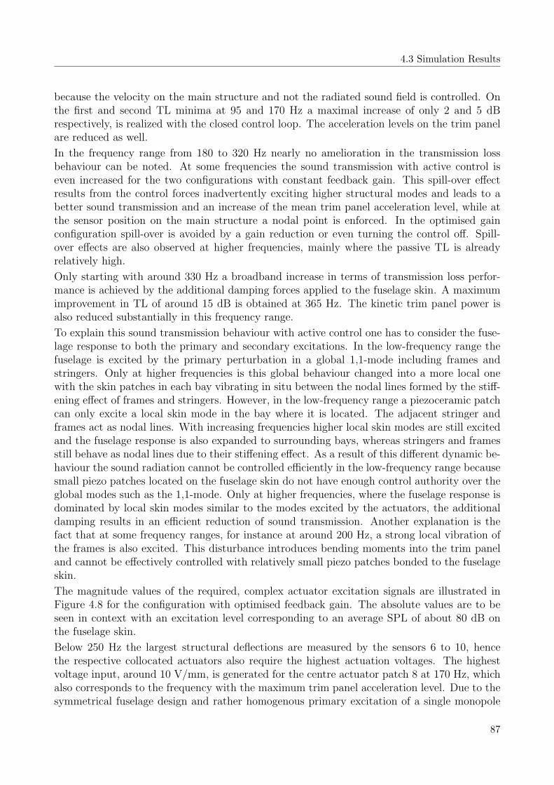
4.3 Simulation Results
because the velocity on the main structure and not the radiated sound field is controlled. Onthe first and second TL minima at 95 and 170 Hz a maximal increase of only 2 and 5 dBrespectively, is realized with the closed control loop. The acceleration levels on the trim panelare reduced as well.
In the frequency range from 180 to 320 Hz nearly no amelioration in the transmission lossbehaviour can be noted. At some frequencies the sound transmission with active control iseven increased for the two configurations with constant feedback gain. This spill-over effectresults from the control forces inadvertently exciting higher structural modes and leads to abetter sound transmission and an increase of the mean trim panel acceleration level, while atthe sensor position on the main structure a nodal point is enforced. In the optimised gainconfiguration spill-over is avoided by a gain reduction or even turning the control off. Spill-over effects are also observed at higher frequencies, mainly where the passive TL is alreadyrelatively high.
Only starting with around 330 Hz a broadband increase in terms of transmission loss perfor-mance is achieved by the additional damping forces applied to the fuselage skin. A maximumimprovement in TL of around 15 dB is obtained at 365 Hz. The kinetic trim panel power isalso reduced substantially in this frequency range.
To explain this sound transmission behaviour with active control one has to consider the fuse-lage response to both the primary and secondary excitations. In the low-frequency range thefuselage is excited by the primary perturbation in a global 1,1-mode including frames andstringers. Only at higher frequencies is this global behaviour changed into a more local onewith the skin patches in each bay vibrating in situ between the nodal lines formed by the stiff-ening effect of frames and stringers. However, in the low-frequency range a piezoceramic patchcan only excite a local skin mode in the bay where it is located. The adjacent stringer andframes act as nodal lines. With increasing frequencies higher local skin modes are still excitedand the fuselage response is also expanded to surrounding bays, whereas stringers and framesstill behave as nodal lines due to their stiffening effect. As a result of this different dynamic be-haviour the sound radiation cannot be controlled efficiently in the low-frequency range becausesmall piezo patches located on the fuselage skin do not have enough control authority over theglobal modes such as the 1,1-mode. Only at higher frequencies, where the fuselage response isdominated by local skin modes similar to the modes excited by the actuators, the additionaldamping results in an efficient reduction of sound transmission. Another explanation is thefact that at some frequency ranges, for instance at around 200 Hz, a strong local vibration ofthe frames is also excited. This disturbance introduces bending moments into the trim paneland cannot be effectively controlled with relatively small piezo patches bonded to the fuselageskin.
The magnitude values of the required, complex actuator excitation signals are illustrated inFigure 4.8 for the configuration with optimised feedback gain. The absolute values are to beseen in context with an excitation level corresponding to an average SPL of about 80 dB onthe fuselage skin.
Below 250 Hz the largest structural deflections are measured by the sensors 6 to 10, hencethe respective collocated actuators also require the highest actuation voltages. The highestvoltage input, around 10 V/mm, is generated for the centre actuator patch 8 at 170 Hz, whichalso corresponds to the frequency with the maximum trim panel acceleration level. Due to thesymmetrical fuselage design and rather homogenous primary excitation of a single monopole
87
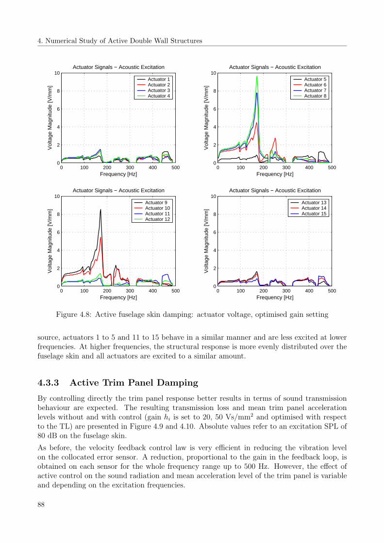
4. Numerical Study of Active Double Wall Structures
0 100 200 300 400 5000
2
4
6
8
10Actuator Signals − Acoustic Excitation
Frequency [Hz]
Vol
tage
Mag
nitu
de [V
/mm
]
Actuator 1Actuator 2Actuator 3Actuator 4
0 100 200 300 400 5000
2
4
6
8
10Actuator Signals − Acoustic Excitation
Frequency [Hz]
Vol
tage
Mag
nitu
de [V
/mm
]
Actuator 5Actuator 6Actuator 7Actuator 8
0 100 200 300 400 5000
2
4
6
8
10Actuator Signals − Acoustic Excitation
Frequency [Hz]
Vol
tage
Mag
nitu
de [V
/mm
]
Actuator 9Actuator 10Actuator 11Actuator 12
0 100 200 300 400 5000
2
4
6
8
10Actuator Signals − Acoustic Excitation
Frequency [Hz]
Vol
tage
Mag
nitu
de [V
/mm
]Actuator 13Actuator 14Actuator 15
Figure 4.8: Active fuselage skin damping: actuator voltage, optimised gain setting
source, actuators 1 to 5 and 11 to 15 behave in a similar manner and are less excited at lowerfrequencies. At higher frequencies, the structural response is more evenly distributed over thefuselage skin and all actuators are excited to a similar amount.
4.3.3 Active Trim Panel Damping
By controlling directly the trim panel response better results in terms of sound transmissionbehaviour are expected. The resulting transmission loss and mean trim panel accelerationlevels without and with control (gain hi is set to 20, 50 Vs/mm2 and optimised with respectto the TL) are presented in Figure 4.9 and 4.10. Absolute values refer to an excitation SPL of80 dB on the fuselage skin.
As before, the velocity feedback control law is very efficient in reducing the vibration levelon the collocated error sensor. A reduction, proportional to the gain in the feedback loop, isobtained on each sensor for the whole frequency range up to 500 Hz. However, the effect ofactive control on the sound radiation and mean acceleration level of the trim panel is variableand depending on the excitation frequencies.
88

4.3 Simulation Results
0 50 100 150 200 250 300 350 400 450 5000
5
10
15
20
25
30
35
40
45
50Transmission Loss − Acoustic Excitation
Frequency [Hz]
Tra
nsm
issi
on L
oss
[dB
]Without controlWith control − optimized gainWith control − gain 20 Vs/mm2
With control − gain 50 Vs/mm2
Figure 4.9: Active trim panel damping: transmission loss, with and without control
0 50 100 150 200 250 300 350 400 450 500−10
−5
0
5
10
15
20
25
30Mean Acceleration − Acoustic Excitation
Frequency [Hz]
Acc
eler
atio
n M
agni
tude
[dB
(m/s
2 )]
Without controlWith control − optimized gainWith control − gain 20 Vs/mm2
With control − gain 50 Vs/mm2
Figure 4.10: Active trim panel damping: mean trim panel acceleration, with and withoutcontrol
89

4. Numerical Study of Active Double Wall Structures
Up to 430 Hz a broadband increase in transmission loss is achieved in the model by controllingthe trim panel response. The first TL minimum at 95 Hz is increased by around 20 dB, howeveron the second peak only a reduction of about 3 dB is obtained. At higher frequencies gains inTL of up to 9 or 7 dB are obtained on frequencies that exhibit a relatively low transmissionloss, as for instance at 250 or respectively 365 Hz. This reduction in sound radiation is mainlydue to the increased damping on the trim panel and the resulting decrease in vibration energy,as shown by the overall acceleration level in Figure 4.10. Comparing the results with thoseobtained with the active skin damping concept, a significant better increase in TL is achievedfor the frequency range below 330 Hz (except for 170 Hz).
The acoustic and structural results indicate that spill-over problems also occur with the activetrim panel damping concept, mainly on frequencies having already a low radiation efficiencyand high transmission loss. To avoid diminutions in transmission loss, control is thereforeturned off in the frequency ranges of 120, 450 and 500 Hz.
With increasing frequencies the acoustic benefit from the active trim panel control is reducedand vanishes completely for frequencies above 450 Hz. Although a substantial control reduc-tion is still obtained locally on the error sensors, the overall structural trim panel and soundradiation behaviour depends on too many degrees of freedom and thus becomes too complexto be controlled with the present actuator concept. The control enforces a nodal point at eachsensor, but the remaining, uncontrolled areas of the panel are no longer affected by the controlor even excited to a greater extent than without control. To increase the efficiency at higherfrequencies a different actuator setup, compromising more and smaller piezo patches, wouldbe required.
The magnitude of the actuator voltage, resulting from the optimised feedback gain setting,is shown in Figure 4.11. In comparison to the active skin damping concept, higher actuationvoltages are required with active trim panel damping. The largest signals are generated foractuators 3 and 11 with around 16 V/mm at 170 Hz. Above 300 Hz the voltage is reduced tolevels well below 2 V/mm on all actuators.
4.3.4 Active Trim Panel Attachments
The main simulation results for the active attachment elements are shown in Figure 4.12 and4.13 in terms of sound transmission loss and mean trim panel acceleration using the acousticmonopole source as the primary perturbation source.
Each of the figures contains the resulting information from two different configurations withoutcontrol (structure fitted with active and rigid attachment elements). Two different configura-tions are also available for the analysis of the closed-loop behaviour with LMS control. Onevariant represents the results from the transmission loss optimisation process (denoted withAAE - with control) that is obtained from the six sensor setup listed in Table 4.4. For the sec-ond controlled configuration, abbreviated with AAE - optimal control, the hypothetical LMScontrol loop containing the entire trim panel response as error signal is used.
The simulation results indicate that by controlling the trim panel response with the activeattachment elements, sound transmission through the aircraft sidewall section is considerablyreduced over nearly the whole frequency range (except for 120 and 460 Hz where no ameliora-tion is obtained with the examined sensor configurations). The first minimum in transmission
90

4.3 Simulation Results
0 100 200 300 400 5000
2
4
6
8
10
12
14
16Actuator Signals − Acoustic Excitation
Frequency [Hz]
Vol
tage
Mag
nitu
de [V
/mm
]
Actuator 1Actuator 2Actuator 3Actuator 4
0 100 200 300 400 5000
2
4
6
8
10
12
14
16Actuator Signals − Acoustic Excitation
Frequency [Hz]
Vol
tage
Mag
nitu
de [V
/mm
]
Actuator 5Actuator 6Actuator 7
0 100 200 300 400 5000
2
4
6
8
10
12
14
16Actuator Signals − Acoustic Excitation
Frequency [Hz]
Vol
tage
Mag
nitu
de [V
/mm
]
Actuator 8Actuator 9Actuator 10
0 100 200 300 400 5000
2
4
6
8
10
12
14
16Actuator Signals − Acoustic Excitation
Frequency [Hz]
Vol
tage
Mag
nitu
de [V
/mm
]Actuator 11Actuator 12Actuator 13
Figure 4.11: Active trim panel damping: actuator voltage, optimised gain setting
loss occurring at 92 Hz disappears totally with control. With the secondary forces and momentsintroduced by the actuators on each attachment point, the 1,1-mode on the trim panel can belargely suppressed and the mean trim panel acceleration and sound radiation are reduced by30 and more than 35 dB respectively. On the second peak at 167 Hz an amelioration of 10 dBis obtained in TL, whereas at 245 Hz the transmission loss is increased from 3,5 dB up to22 dB with control. With further increasing frequency up to 450 Hz a broadband attenuationof about 5 to 10 dB in sound transmission is achieved with the active attachment actuators.
At higher frequencies the general tendency is that the benefit from control decreases and theefficiency limit of the selected actuator concept is apparently reached. The modal density onthe trim panel increases and the dynamic response becomes too complex and an efficient controlwith only twelve degrees of freedom for the secondary signals is not possible anymore. This canbe seen by the fact that with the optimal trim panel control, having around 100 times moreerror information from the trim panel at its disposal than the normal LMS algorithm (andthus representing an optimal solution in terms of trim panel acceleration with the availabletwelve actuation degrees of freedom), no significant better results are achieved above 350 Hz.Nevertheless, the transmission loss behaviour is still improved at frequencies above 450 Hz.
91

4. Numerical Study of Active Double Wall Structures
0 50 100 150 200 250 300 350 400 450 5000
10
20
30
40
50
60Transmission Loss − Acoustic Excitation
Frequency [Hz]
Tra
nsm
issi
on L
oss
[dB
]AAE − without controlAAE − with controlAAE − optimal controlRigid Attachment
Figure 4.12: Active attachment elements: transmission loss, with and without control
0 50 100 150 200 250 300 350 400 450 500−10
−5
0
5
10
15
20
25
30Mean Acceleration − Acoustic Excitation
Frequency [Hz]
Acc
eler
atio
n M
agni
tude
[dB
(m/s
2 )]
AAE − without controlAAE − with controlAAE − optimal controlRigid Attachment
Figure 4.13: Active attachment elements: mean trim panel acceleration, with and withoutcontrol
92

4.3 Simulation Results
The reduction in sound radiation is mainly obtained by a large decrease of the mean trim panelacceleration as illustrated in Figure 4.13. This signifies that the active structural control worksmainly in an active damping mode, reducing the overall kinetic power of the trim panel. Modalrestructuring, characterised by an increase in vibration power, does not occur with the LMScontrol in the considered frequency range. In terms of acceleration reduction the configurationwith the hypothetical, optimal trim panel control represents the best possible global solutionand hence a lower bound that cannot be further decreased with the active attachment elementsand available twelve degrees of freedom.
Figure 4.14 shows which out of the six sensor concepts listed in Table 4.4 is chosen in respectto the optimum sound transmission behaviour. The results depend on the excitation frequencyand it can be seen that no single layout is preferred over the others. On two frequencies (120and 460 Hz) the control is switched off to avoid spill-over. Furthermore, it should be mentionedthat the sensor selection is also dependent on the structural properties and the type of primaryexcitation and that the presented results do not represent the absolute optimal solution thatcan be achieved with such a type of control.
0 50 100 150 200 250 300 350 400 450 500Concept 1
Concept 2
Concept 3
Concept 4
Concept 5
Concept 6
Control OFF
Frequency [Hz]
Sensor Selection − Acoustic Excitation
Figure 4.14: Active attachment elements: selected sensor concepts
The magnitude of the complex actuation signals derived with the LMS algorithm is shownin Figure 4.15 (configuration: AAE - with control). The maximum values are reached onactuators 1, 4 and 10 with around 80 V at 170 Hz. In this frequency range both the overallacceleration level on the panel and the sound transmission exhibit a global maximum. As in theprevious example, the absolute values are calculated for a perturbation source strength givinga mean sound pressure level of 80 dB on the incident panel. By assuming a more realisticexcitation level of 100 dB, all absolute quantities must be multiplied by a factor of ten. Thus,a maximum voltage of around 800 V would be required to control the structural system. As
93

4. Numerical Study of Active Double Wall Structures
the maximum voltage that can be applied to the Thunder elements is limited to 240 V, suchan excitation is not possible without accepting a destruction of the actuators.
Figure 4.14 indicates that in the frequency range, where the actuator voltage limit would beexceeded, sensor concepts three to six are selected by the TL optimisation process. They havein common that only sensors placed directly on the trim panel are used in the control loop aserror signal. If, instead, one of the concepts with error sensors integrated on the attachmentelements would be used, a considerable reduction in the actuator voltage could be obtainedand even for an excitation strength of 100 dB the voltage limit of 240 V would not be exceededas the error signal used on the attachment elements have the effect of providing an additionalcontrol effort reduction. On the other hand, this would also reduce the control perfomance,but for instance on the three global minimum TL values at 92, 167 and 245 Hz gains of about30, 5 and 9 dB respectively in TL could still be realized with such a type of control. In thiscase the actuators would be excited up to a level of about 80% of their maximum voltage.
0 100 200 300 400 5000
10
20
30
40
50
60
70
80
90Actuator Signals − Acoustic Excitation
Frequency [Hz]
Vol
tage
Mag
nitu
de [V
]
Actuator 1Actuator 2Actuator 3
0 100 200 300 400 5000
10
20
30
40
50
60
70
80
90Actuator Signals − Acoustic Excitation
Frequency [Hz]
Vol
tage
Mag
nitu
de [V
]
Actuator 4Actuator 5Actuator 6
0 100 200 300 400 5000
10
20
30
40
50
60
70
80
90Actuator Signals − Acoustic Excitation
Frequency [Hz]
Vol
tage
Mag
nitu
de [V
]
Actuator 7Actuator 8Actuator 9
0 100 200 300 400 5000
10
20
30
40
50
60
70
80
90Actuator Signals − Acoustic Excitation
Frequency [Hz]
Vol
tage
Mag
nitu
de [V
]
Actuator 10Actuator 11Actuator 12
Figure 4.15: Active attachment elements: actuator voltage
In order to evaluate how the electrical actuation power is transformed into normal z-translationsand x,y-rotations, the actuator command signal is transformed into an appropriate coordinate
94

4.3 Simulation Results
system for each attachment element. The electrical power P is defined by the product ofactuator voltage U and current I. The power magnitude is proportional to the square of theactuator voltage, because the piezoceramic behaves electrically as capacity with the actuatorcurrent being proportional to the applied voltage:
PActuator (s) = U (s) · I (s) ∼ U2 (s) . (4.1)
The normal translation part of the actuator excitation can be calculated from the complexcommand signal parts, which are in phase:
Utranslation (s) = a · (U1 + U2 + U3) . (4.2)
The rotational parts around the orthogonal axes x and y are derived by using the geometricalsetup illustrated in Figure 4.3:
Urot,x = −b · U1 + b · sin 30 · U2 + b · sin 30 · U3 ,
Urot,y = −b · cos 30 · U1 + b · cos 30 · U3 . (4.3)
In matrix form equation 4.2 and 4.3 can be rewritten as:
Utranslation
Urot,x
Urot,y
=
a a a−b b · sin 30 b · sin 30
0 −b · cos 30 b · cos 30
·
U1
U2
U3
⇔ UT (s) = M · U (s) . (4.4)
To satisfy the principle of energy conservation, the transformation must fulfil the followingcondition:
UTT · UT = UT · U . (4.5)
Taking into account expression 4.4 leads to:
UTT · UT = (M · U)T ·M · U = UT ·MT ·M · U . (4.6)
Condition 4.5 is only satisfied when the term MTM equals the unity matrix. With thiscondition parameter a and b are derived as:
a =1√3
and b =
√2
3. (4.7)
The final power ratios for the normal translatory and rotational components in the transformedsystem with respect to the total power are given for each attachment element by the followingrelation:
95
4. Numerical Study of Active Double Wall Structures
Ltranslation =|Utranslation|2∑12
i=1 U2i
, Lrot,x =|Urot,x|2∑12
i=1 U2i
, Lrot,y =|Urot,y|2∑12
i=1 U2i
. (4.8)
The power ratios obtained with equation 4.8 are plotted in Figure 4.16 for each attachment ele-ment. Due to the non-symmetrical primary excitation on the fuselage skin and non-symmetricallayout of sensors the actuation power is not evenly distributed on each attachment element.For instance at frequencies up to 100 Hz the attachment element AAE 1, being the nearest tothe primary excitation source, requires more than 60% of the total actuation power. Other-wise, for most of the frequency range, the actuation signal is mainly dominated by a rotationin the x-direction, which also corresponds to the direction of the frames and is perpendicularto the direction with the highest bending stiffness. Rotations y-direction are also stronglyexcited at some frequencies, whereas normal translations are only generated around 130 and450 Hz. These results confirm the assumption from the preliminary investigations that bothtranslatory and rotational perturbation components must be controlled in order to achieve asubstantial reduction in sound transmission.
Power Ratio − AAE 1
Frequency [Hz]
Pow
er R
atio
[%]
0 100 200 300 400 5000
20
40
60
80
100z
transx
roty
rot
Power Ratio − AAE 2
Frequency [Hz]
Pow
er R
atio
[%]
0 100 200 300 400 5000
20
40
60
80
100
Power Ratio − AAE 3
Frequency [Hz]
Pow
er R
atio
[%]
0 100 200 300 400 5000
20
40
60
80
100Power Ratio − AAE 4
Frequency [Hz]
Pow
er R
atio
[%]
0 100 200 300 400 5000
20
40
60
80
100
Figure 4.16: Active attachment elements: translatory and rotational actuation powercomponents
96

4.4 Analysis and Comparison
In contrast to the simulation study presented by Gardonio and Elliott [Gardonio98], goodresults are obtained with the active attachment elements because translatory and rotationalcontrol forces can be excited at each trim panel attachment point and additional sensors locatedon the trim panel and monitoring the sound radiation are used in the control loop.
4.4 Analysis and Comparison
As the primary goal of all three active technologies is to increase the transmission loss ofthe fuselage section with respect to various primary perturbations in the lower frequency range(buzz-saw noise, jet noise, TBL noise and structure-borne noise), a direct comparison of the bestresults obtained with each control concept is made in order to determine the technology havingthe highest potential for an active structural control application. For this purpose simulationresults obtained with three different primary excitations of the fuselage skin (acoustic monopolesource, diffuse sound field and point force excitation) are analysed. The same setup as inChapter 3.4 is used for the primary sources.
Figure 4.17 and 4.18 summarize the acoustic and structural results for the monopole excitation.The direct comparison reveals that the concept with active attachment elements is by fargiving the best sound transmission behaviour for the considered frequency range. Only at twofrequency ranges, 330 to 380 Hz and 440 to 470 Hz, better acoustic results are obtained withthe active damping technology applied to the fuselage skin, as at those particular frequenciesthe sound transmission is dominated by locally vibrating skin patches. In terms of trim panelacceleration the best results are also obtained with the active attachment elements.
For the diffuse field and point force primary excitations the feedback gain optimisation outputfor the active damping configurations and the frequency-dependant sensor selection used withthe active attachment elements are different to ones selected for the monopole excitation.However, very similar simulation results are achieved for the acoustic and structural quantities.The respective results obtained with the diffuse field primary excitation are presented in Figure4.19 for the TL and in Figure 4.20 for the mean trim panel acceleration, whereas in Figure 4.21and 4.22 the total sound power radiated by the trim panel and its mean acceleration level areshown for the point force perturbation. In both cases on nearly the whole frequency range thebest TL results, respectively decrease in radiated sound power, are obtained with the activeattachment technology.
The collocated actuators and sensor of the active damping concepts were also tested in combi-nation with the LMS control algorithm. Typically such type of control results in higher localcontrol reductions at the error sensors than the ones obtained with a local velocity feedbackcontrol. However, in terms of transmission loss increase, no amelioration in comparison to theones obtained with the feedback variants was achieved. Hence, these results are not presentedin this study.
In addition to the ASAC control performed with all active technologies, an evaluation of anactive noise control configuration was also carried out. In this mode the acceleration error sen-sors are replaced with an array of microphones located either in the cavity or in the acousticnear-field radiated by the trim panel. In both cases the control loop is driven with the LMSalgorithm. By controlling directly the acoustic sound field superior acoustic results in compar-ison to an active structural acoustic control are obtained. Yet, this control concept was not
97

4. Numerical Study of Active Double Wall Structures
0 50 100 150 200 250 300 350 400 450 5000
10
20
30
40
50
60Transmission Loss − Acoustic Excitation
Frequency [Hz]
Tra
nsm
issi
on L
oss
[dB
]Rigid AttachmentAAE − without controlAAE − with controlActive Fuselage Skin DampingActive Trim Panel Damping
Figure 4.17: Comparison of resulting TL (active attachment elements, fuselage skin and trimpanel damping), with and without control, acoustic monopole excitation
0 50 100 150 200 250 300 350 400 450 500−10
−5
0
5
10
15
20
25
30Mean Trim Panel Acceleration − Acoustic Excitation
Frequency [Hz]
Acc
eler
atio
n M
agni
tude
[dB
(m/s
2 )]
Rigid AttachmentAAE − without controlAAE − with controlActive Fuselage Skin DampingActive Trim Panel Damping
Figure 4.18: Mean trim panel acceleration level (active attachment elements, fuselage skinand trim panel damping), with and without control, acoustic monopole excitation
98

4.4 Analysis and Comparison
0 50 100 150 200 250 300 350 400 450 5000
10
20
30
40
50
60Transmission Loss − Diffuse Acoustic Excitation
Frequency [Hz]
Tra
nsm
issi
on L
oss
[dB
]Rigid AttachmentAAE − without controlAAE − with controlActive Fuselage Skin DampingActive Trim Panel Damping
Figure 4.19: Comparison of resulting TL (active attachment elements, fuselage skin and trimpanel damping), with and without control, acoustic diffuse excitation
0 50 100 150 200 250 300 350 400 450 500−30
−25
−20
−15
−10
−5
0
5
10
15
20
25Mean Trim Panel Acceleration − Diffuse Acoustic Excitation
Frequency [Hz]
Acc
eler
atio
n M
agni
tude
[dB
(m/s
2 )]
Rigid AttachmentAAE − without controlAAE − with controlActive Fuselage Skin DampingActive Trim Panel Damping
Figure 4.20: Mean trim panel acceleration level (active attachment elements, fuselage skinand trim panel damping), with and without control, acoustic diffuse excitation
99

4. Numerical Study of Active Double Wall Structures
0 50 100 150 200 250 300 350 400 450 50030
40
50
60
70
80
90Radiated Acoustic Power − Point Force Excitation
Frequency [Hz]
Rad
iate
d A
cous
tic P
ower
[dB
]
Rigid AttachmentAAE − without controlAAE − with controlActive Fuselage Skin DampingActive Trim Panel Damping
Figure 4.21: Comparison of radiated sound power (active attachment elements, fuselage skinand trim panel damping), with and without control, point force excitation
0 50 100 150 200 250 300 350 400 450 500−10
0
10
20
30
40
50Mean Trim Panel Acceleration − Point Force Excitation
Frequency [Hz]
Acc
eler
atio
n M
agni
tude
[dB
(m/s
2 )]
Rigid AttachmentAAE − without controlAAE − with controlActive Fuselage Skin DampingActive Trim Panel Damping
Figure 4.22: Mean trim panel acceleration level (active attachment elements, fuselage skinand trim panel damping), with and without control, point force excitation
100

4.5 Conclusions
pursued, as the trim panel is driven in an efficient radiation mode, which results in far highertrim panel acceleration levels than without control and thus could cause structural problemsin the worst case. Also the actuation effort needed for this type of control is much increasedin comparison to the various ASAC control configurations. Furthermore, in reality it might beproblematic or even impossible to place microphones in front of the radiating structure.
The control in the cavity is aimed at reducing the cavity sound pressure and thus the loadingand sound radiation of the trim panel. In combination with the d31-actuators placed on thefuselage skin this sensor concept showed some promising results at frequencies below 200 Hz,but at higher frequencies sound transmission is increased due to spill-over effects and strongexcitation of higher cavity modes. An increased actuation effort in contrast to the structuralcontrol approach is also required. The active attachment elements and actuators placed onthe trim panel are not suited to a cavity pressure control as, besides the obtained reductionin cavity pressure, which is indirectly controlled by the trim panel behaviour in this case, anincrease of the mean acceleration level and thus of the sound radiation is typically excited bythe actuators as well.
4.5 Conclusions
In this chapter the performance of three different actuator and sensor concepts aimed at reduc-ing the sound transmission through aircraft sidewall sections at low frequencies was numericallyanalysed for various primary excitations. The simulation model is based on a generic, planedouble wall fuselage section and takes into account structure-borne as well as airborne noisepropagation. An ASAC system is used to control the dynamic response of the structure to anexternal primary perturbation of the fuselage skin and to improve the transmission loss.
Two of the active systems are intended to increase the structural damping and make use ofd31-piezo patches either bonded to the fuselage skin or the trim panel. In this configurationthe controller is implemented as local velocity feedback algorithm in combination with collo-cated actuators and unidirectional acceleration sensors. In general, it is demonstrated by thesimulation results that an increase in transmission loss can be obtained with actuator sensorpairs located directly on the trim panel. The additional damping forces reduce the mean accel-eration level on the trim panel, which in turn is correlated to the total radiated sound power.On some frequencies the sound transmission through the double wall is essentially determinedby locally vibrating fuselage skin modes. At those frequencies better results in terms of TL in-crease are achieved with the actuators placed on the fuselage skin. However, this configurationis not adapted to low-frequency perturbations as the actuators do not have a sufficient controlauthority on global modes, which are mainly excited on the fuselage skin at low frequencies.
The third active technology is based on active trim panel attachment elements, which replacethe standard shock mounts used to attach the trim panel on the main fuselage. The actuatorsutilize the piezoelectric d31-bending effect and through a particular design of the elementsboth normal translatory and rotational perturbation components induced at the attachmentpoints can be controlled. The controller is implemented as LMS algorithm and error signalsfrom acceleration sensors integrated within the attachment elements and the trim panel arecontrolled. In the simulation model, out of the three proposed active technologies, the activeattachment approach gives the best control performance in terms of acoustic and structural
101

4. Numerical Study of Active Double Wall Structures
results. Furthermore, if the sound transmission is dominated by structure-borne noise, theactive attachment elements also represent the most adequate active technology.
Taking into consideration these simulation results, the active damping systems do not seem torepresent suitable solutions for the improvement of the transmission loss of aircraft sidewallsections. Further experimental investigations will focus on the development and testing ofprototype active attachment elements.
102
Chapter 5
Experimental Study
The experimental results, which were achieved with a prototype control and actuator system,are presented in this chapter. In general the basic layout resembles the simulation modeldescribed in the previous chapter. A plane section of a generic aircraft double wall structure,consisting of a main fuselage and trim panel, is installed between two acoustic chambers. Thechamber facing the fuselage skin panel is used for the excitation of the structure, which iseither done acoustically by loudspeakers or with a mechanical point force, whereas in thechamber facing the trim panel the global and local sound power transmitted by the structureis measured.
The trim panel is attached to the fuselage via four active attachment elements, which areused to control the dynamic response and sound radiation of the trim panel. The controlalgorithm is implemented on a DSP system, driving the actuators in such way that an errorvibration level, measured on the structure, is minimized. The performance and efficiency of theactive structural acoustic control system is evaluated against various deterministic and randomdisturbances. The deterministic perturbation represents a harmonic noise source similar to abuzz-saw noise excitation, whereas a random excitation like the turbulent boundary layer noiseis simulated by band-filtered white noise disturbances.
5.1 Design of a Prototype Active Attachment Element
Based on the simulation results obtained with the fuselage trim-panel model presented inChapter 4, a Thunder actuator for a prototype active attachment element has been designedand manufactured. The design is derived from the commercially available Thunder actuatorsTH-10R and features a similar composite lay-up and PZT properties. The dimensions of themetal substrate and PZT layer are changed to the values listed in Table 5.1. A photo of thebasic element is shown on the left side of Figure 5.1. In contrast to the model TH-10R, nomounting slots are provided on the tabs, because the element will be used in a pure clamshellconfiguration. Furthermore, the actuator design includes a hole in the centre of the actuator.This hole accepts screws up to a size of M2.5 and is used to connect the clamshell actuator unitto the mounting plate through a spacer clamping-sleeve construction. The actuator top layeris made of copper and provides a good soldering base for the attachment of the electrodes.The maximum input voltage at which the Thunder elements may be operated is 480 V peak

5. Experimental Study
to peak. This voltage is equivalent to an electric field strength of around 2360 V/mm acrossthe thickness of the PZT layer.
Table 5.1: Specifications of the basic Thunder element
Thunder Specifications
Overall dimensions: 32,0 x 19,0 x 1,1 mm
PZT-dimensions: 23,0 x 18,0 mm
Composite thickness: 0,43 mm
Substrate layer thickness: 0,20 mm
PZT layer thickness: 0,20 mm
ø mounting hole substrate: 2,6 mm
ø mounting hole PZT: 6,0 mm
Weight: 1,4 g
Capacity: 18 nF
Max. voltage (Vpp): 480 V
Typical displacement∗: approx. 1 mm
Blocked force: not available
∗ clamped support on one side, maximum input voltage,quasi-static deflection peak to peak of the free tip at 1 Hz
The actuator unit used in the active attachment element consists of two Thunder actuators andtwo clamshell mounts. Integrated in each clamshell mount is a 0,2 mm thick and 3 mm deepslot, which is used to retain the Thunder elements on their free tabs, thus providing a clampedsupport that holds the actuator end at a fixed angle when the device tries to bend. However,the mounting elements are not prevented from moving relative to each other when the wholeactuator unit flexes. Hence, a pure translation perpendicular to the PZT surface is generatedat the centre of the actuator device. The mounting elements are manufactured in steel byan electrical discharge machining process. As adhesive the two-part epoxy resin system CibaEpocast 52-A and B is used. The resulting spacing between the Thunder elements is 5,9 mm.An image of the finished clamshell element is reproduced on the right side of Figure 5.1 withthe spacer clamping-sleeve element already in place. The overall dimensions of the clamshellelement are 34 by 19 by 8,3 mm. An additional technical drawing of the basic actuator unit ispresented in Annex B.
To demonstrate the design and construction of the active attachment element, a picture withthe individual components prior to assembling and an exploded view of the actuator elementare shown in Figure 5.2 and 5.3. The mounting plates are made from 3 mm thick aluminiumand must provide a stiff support for both the actuators and the error sensors. Otherwise thepiezoelectric actuator would not couple efficiently into the host structure and the error signalswould not correlate with the actual disturbances. An FEM normal modes analysis of themounting plate (free boundary conditions) showed that the first bending mode occurs only at3,8 kHz. Therefore, the hexagonal shape already used in the simulation model is retained. Thewidth across the flat side of the hexagon is 62 mm. Since the mounting plate is electricallyconnected to the actuator’s substrate layer, it also serves as common electric ground for thepower supply.
104

5.1 Design of a Prototype Active Attachment Element
Figure 5.1: Basic Thunder element and actuator unit in clamshell configuration
Figure 5.2: Components of an active attachment element
Three actuators as well as three error sensors are disposed axially symmetric by 120 degreesaround the centre of the mounting plate. For the actuators the leverage distance to the centrepoint is 21,5 mm, whereas the radius for the error sensors is 26,5 mm. The unidirectionalacceleration sensors of the type PCB M353B65 are directly integrated in the upper mountingplate with M3 screw threads provided in the plate. The active attachment element is clampedto the host structure with a similar spacer clamping-sleeve construction as on the clamshellelements by using M4 screws. To ensure that the elements can be mounted inside a doublewall partition that may not be accessible from outside, the attachment screws are glued tothe mounting plate. Figure 5.4 shows a fully assembled and functional prototype. The overallheight is 22,6 mm and the total weight sums up to 98 g (without taking into account cablesfor power supply and acceleration sensors). A technical drawing of the prototype attachmentelement is also reproduced in Annex B.
Figure 5.5 shows the measured complex frequency-response function in terms of accelerationper applied unity voltage for an active attachment element. The attachment element is excitedby a voltage applied to the first actuator unit and the response of the three acceleration sensors
105
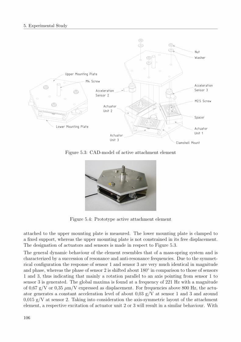
5. Experimental Study
M4 Screw
Washer
Acceleration
Sensor 3
M2.5 Screw
Nut
Actuator
Unit 2
Lower Mounting Plate
Spacer
Upper Mounting Plate
Actuator
Unit 3
Actuator
Unit 1
Acceleration
Sensor 2
Clamshell Mount
Figure 5.3: CAD-model of active attachment element
Figure 5.4: Prototype active attachment element
attached to the upper mounting plate is measured. The lower mounting plate is clamped toa fixed support, whereas the upper mounting plate is not constrained in its free displacement.The designation of actuators and sensors is made in respect to Figure 5.3.
The general dynamic behaviour of the element resembles that of a mass-spring system and ischaracterized by a succession of resonance and anti-resonance frequencies. Due to the symmet-rical configuration the response of sensor 1 and sensor 3 are very much identical in magnitudeand phase, whereas the phase of sensor 2 is shifted about 180 in comparison to those of sensors1 and 3, thus indicating that mainly a rotation parallel to an axis pointing from sensor 1 tosensor 3 is generated. The global maxima is found at a frequency of 221 Hz with a magnitudeof 0,67 g/V or 0,35 µm/V expressed as displacement. For frequencies above 800 Hz, the actu-ator generates a constant acceleration level of about 0,03 g/V at sensor 1 and 3 and around0,015 g/V at sensor 2. Taking into consideration the axis-symmetric layout of the attachmentelement, a respective excitation of actuator unit 2 or 3 will result in a similar behaviour. With
106

5.1 Design of a Prototype Active Attachment Element
0 200 400 600 800 1000 1200 1400 160010
−3
10−2
10−1
100
Acceleration per Unity Voltage − Magnitude
Frequency [Hz]
Acc
eler
atio
n / V
olta
ge [g
/V]
Acc. Sensor 1Acc. Sensor 2Acc. Sensor 3
0 200 400 600 800 1000 1200 1400 1600
−150
−100
−50
0
50
100
150
Acceleration per Unity Voltage − Phase
Frequency [Hz]
Pha
se [°
]
Acc. Sensor 1Acc. Sensor 2Acc. Sensor 3
Figure 5.5: Measured actuator response per unity voltage applied to actuator unit 1
an appropriate simultaneous excitation of all three actuator units, it is possible to excite an ar-bitrary relative displacement between the upper and lower mounting plate, which is composedof a normal translation and two perpendicular rotations in the plate’s plane.
This prototype design provides a good starting point for further developments and may beoptimised in terms of size, weight, actuator performance and degree of structural integrationinto the fuselage and trim panel. The displacement and force generated by a single actuator unitare easily scalable for different requirements. The main design variables are the piezoceramicthickness relative to the substrate layer, the length and width of the Thunder element and themounting condition for the clamshell configuration. Thus, with a thicker piezoceramic layer,a greater force will be generated at the expense of the displacement. The actuator width isdirectly proportional to the force and a less stiff mounting condition will provide a greaterdisplacement, but also less force.
The unidirectional force and displacement components generated by a single actuator unitare converted at the trim panel attachment point into a force and two orthogonal moments,respectively a translation and two perpendicular rotations. Whether the active attachmentelement will be mainly a force or displacement actuator depends primarily on the leveragedistance between the force transmitting point of the clamshell device to the mounting pointof the attachment element. With increasing leverage distance the attachment element willgenerate a greater moment and less rotational displacement.
107

5. Experimental Study
5.2 Test Setup and Experimental Methods
The effectiveness of a structural noise and vibration control system based on active trim panelattachments is demonstrated in laboratory scale on a generic aircraft fuselage section installedinto a transmission loss suite between a reverberation and anechoic room. The test structure,measurement method and various types of excitation as well as the control loop implemen-tation are presented in the following chapters. For each single test constellation an intensitymeasurement of the radiating trim panel surface is carried out with and without active control.Thus, the total sound power transmitted through the structure is determined, permitting adirect evaluation of the active control effectiveness.
5.2.1 Test Structure Description
For the evaluation of the active control system a double wall partition consisting of a planegeneric fuselage section combined with a typical trim panel, as depicted on the left side ofFigure 5.6, is used. The fuselage panel is manufactured from a CFRP skin panel reinforcedby five stringers in one direction and two additional CFRP frames in perpendicular direction.The panel meets the TANGO1 specifications for advanced composite airframe structures. TheT-sectioned stringers are structurally fully integrated in the skin panel. In-plane dimensions ofthe skin panel are about 1 by 1 m and the nominal skin thickness is 2,5 mm. Stringer heightis 37 mm and the stringer pitch amounts 175 mm. The C-sectioned carbon fibre frames, alsodesigned to TANGO requirements, are riveted to the skin panel and additional aluminium clipsare used to connect the frames to the stringers. The frame height is 90 mm while the framepitch is 533 mm. The overall weight of the fuselage structure adds up to 8,2 kg.
Trim Panel
Fuselage Skin
Stringer
Frame
Active Attachment ElementAluminium Clip
Figure 5.6: Test structure CAD-model
Two different trim panels, possessing identical in-plane dimensions as the fuselage, are avail-able for various active structural control tests. Both panels are designed as honeycomb coresandwich construction and based on trim panel designs already used in real aircraft. The firstpanel is composed of a 8 mm thick Nomex honeycomb core layer and is reinforced by fabricfibreglass skin sheets on both sides, while a 4 mm thick Nomex honeycomb layer constitutes
1TANGO is a research project within the EU Fifth Framework Programme (FP5).
108
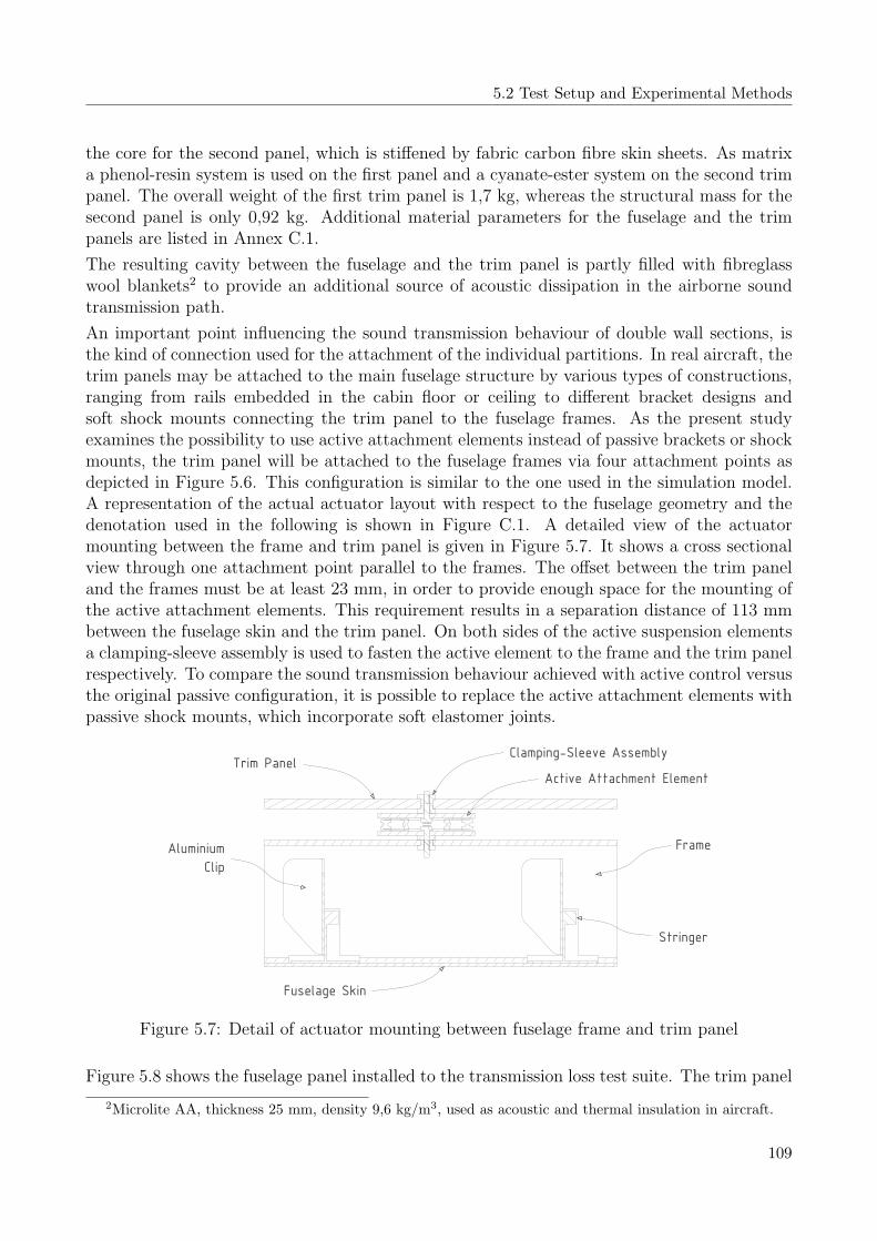
5.2 Test Setup and Experimental Methods
the core for the second panel, which is stiffened by fabric carbon fibre skin sheets. As matrixa phenol-resin system is used on the first panel and a cyanate-ester system on the second trimpanel. The overall weight of the first trim panel is 1,7 kg, whereas the structural mass for thesecond panel is only 0,92 kg. Additional material parameters for the fuselage and the trimpanels are listed in Annex C.1.
The resulting cavity between the fuselage and the trim panel is partly filled with fibreglasswool blankets2 to provide an additional source of acoustic dissipation in the airborne soundtransmission path.
An important point influencing the sound transmission behaviour of double wall sections, isthe kind of connection used for the attachment of the individual partitions. In real aircraft, thetrim panels may be attached to the main fuselage structure by various types of constructions,ranging from rails embedded in the cabin floor or ceiling to different bracket designs andsoft shock mounts connecting the trim panel to the fuselage frames. As the present studyexamines the possibility to use active attachment elements instead of passive brackets or shockmounts, the trim panel will be attached to the fuselage frames via four attachment points asdepicted in Figure 5.6. This configuration is similar to the one used in the simulation model.A representation of the actual actuator layout with respect to the fuselage geometry and thedenotation used in the following is shown in Figure C.1. A detailed view of the actuatormounting between the frame and trim panel is given in Figure 5.7. It shows a cross sectionalview through one attachment point parallel to the frames. The offset between the trim paneland the frames must be at least 23 mm, in order to provide enough space for the mounting ofthe active attachment elements. This requirement results in a separation distance of 113 mmbetween the fuselage skin and the trim panel. On both sides of the active suspension elementsa clamping-sleeve assembly is used to fasten the active element to the frame and the trim panelrespectively. To compare the sound transmission behaviour achieved with active control versusthe original passive configuration, it is possible to replace the active attachment elements withpassive shock mounts, which incorporate soft elastomer joints.
Active Attachment ElementTrim Panel
Frame
Clamping-Sleeve Assembly
Stringer
Fuselage Skin
Aluminium
Clip
Figure 5.7: Detail of actuator mounting between fuselage frame and trim panel
Figure 5.8 shows the fuselage panel installed to the transmission loss test suite. The trim panel
2Microlite AA, thickness 25 mm, density 9,6 kg/m3, used as acoustic and thermal insulation in aircraft.
109

5. Experimental Study
is not yet installed thus making visible the active attachment elements as well as the wiringneeded for the actuator power supply and the acceleration error sensors. Also visible are theglass wool absorption blankets covering the whole fuselage skin apart from the frames.
Figure 5.8: Fuselage panel installed in TL test suite, active attachment elements alreadyinstalled
5.2.2 Transmission Loss Test Facility
Figure 5.9 shows a schematic view of the transmission loss test facility used for the experimentalinvestigation of the structural acoustic control system. The test facility consists of an anechoicchamber, a reverberation room and a transmission loss test window representing the onlyconnection between the two rooms. To avoid a flanking path transmission of energy, bothrooms, the anechoic and reverberation chamber, are structurally isolated from each other andthe rest of the building by an elastic suspension system.
Anechoic
Chamber
219,9 m3 Test Window
Reverberation
Chamber 107,5 m3
Acoustic
Wedges
Detail A
Detail A
Test Panel
Clamping Frame
Wood Fixture
Brick
Wall
Glass WoolWooden Wedge
PU-Foam
Figure 5.9: Schematic plan of the transmission loss test facility and detail of test structureinstallation
The anechoic chamber has inner dimensions of 12,0 m in length, 4,8 m in width and 3,8 m inheight resulting in a volume of 220 m3. The volume of the reverberation room is 108 m3 and
110
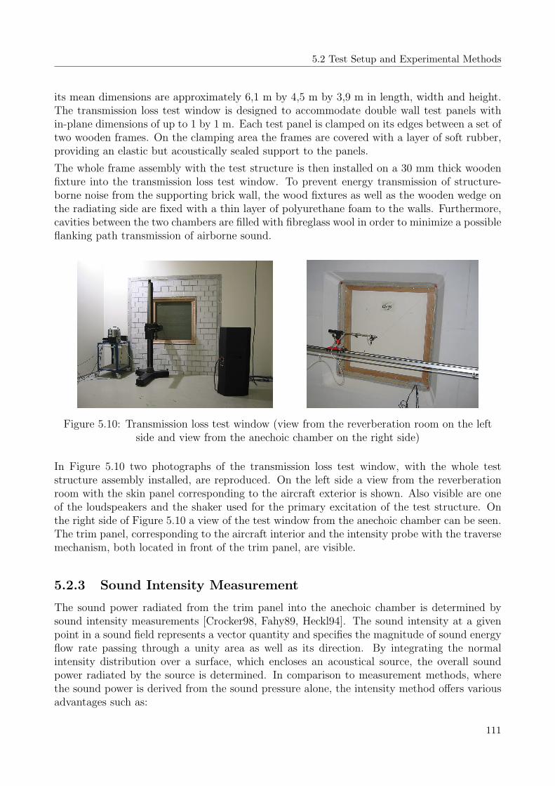
5.2 Test Setup and Experimental Methods
its mean dimensions are approximately 6,1 m by 4,5 m by 3,9 m in length, width and height.The transmission loss test window is designed to accommodate double wall test panels within-plane dimensions of up to 1 by 1 m. Each test panel is clamped on its edges between a set oftwo wooden frames. On the clamping area the frames are covered with a layer of soft rubber,providing an elastic but acoustically sealed support to the panels.
The whole frame assembly with the test structure is then installed on a 30 mm thick woodenfixture into the transmission loss test window. To prevent energy transmission of structure-borne noise from the supporting brick wall, the wood fixtures as well as the wooden wedge onthe radiating side are fixed with a thin layer of polyurethane foam to the walls. Furthermore,cavities between the two chambers are filled with fibreglass wool in order to minimize a possibleflanking path transmission of airborne sound.
Figure 5.10: Transmission loss test window (view from the reverberation room on the leftside and view from the anechoic chamber on the right side)
In Figure 5.10 two photographs of the transmission loss test window, with the whole teststructure assembly installed, are reproduced. On the left side a view from the reverberationroom with the skin panel corresponding to the aircraft exterior is shown. Also visible are oneof the loudspeakers and the shaker used for the primary excitation of the test structure. Onthe right side of Figure 5.10 a view of the test window from the anechoic chamber can be seen.The trim panel, corresponding to the aircraft interior and the intensity probe with the traversemechanism, both located in front of the trim panel, are visible.
5.2.3 Sound Intensity Measurement
The sound power radiated from the trim panel into the anechoic chamber is determined bysound intensity measurements [Crocker98, Fahy89, Heckl94]. The sound intensity at a givenpoint in a sound field represents a vector quantity and specifies the magnitude of sound energyflow rate passing through a unity area as well as its direction. By integrating the normalintensity distribution over a surface, which encloses an acoustical source, the overall soundpower radiated by the source is determined. In comparison to measurement methods, wherethe sound power is derived from the sound pressure alone, the intensity method offers variousadvantages such as:
111
5. Experimental Study
• Measurements can be made in almost every environment and are not restricted to speciallaboratory rooms as anechoic or reverberation chambers.
• A spatial localisation of noise sources is possible, because magnitude and direction of theenergy flow are locally measured.
• Parasitic effects due to the presence of incoherent, static background noise sources aremostly compensated by the measurement method itself and do not contribute to themeasured sound power.
A typical application for sound intensity measurement techniques is the determination of trans-mission loss as described in the European Standard Norm EN ISO 15186-13. Compared to thestandard measurement method, where the transmission loss of a partition is measured betweentwo reverberation rooms [Heckl94], the sound intensity technique is advantageous because:
• The sound transmission behaviour of the partition is evaluated over individual sections.Regions with high intensity can thus be identified and interpreted as locations of noisesources.
• It is possible to detect and quantify possible leaks and flanking path transmission of themeasurement test window.
• The receiving chamber does not need to be calibrated for its reverberation time.
The definition of sound intensity I is given by the product of the sound pressure p and particlevelocity v averaged over a measurement time T :
I = p(t) · v(t) =1
T
∫ T
0
p(t) · v(t) · dt , (5.1)
and indicates the sound power passing through a unity area normal to the particle velocity.Hence, the sound intensity can be integrated over a measurement surface S to yield the totalsound power P passing through that surface:
P =
∫
S
I · dS =
∫
S
p(t) · v(t)dS =1
T
∫
S
∫ T
0
p(t) · v(t) · dt · dS . (5.2)
In practice the above integral is replaced by a numerical summation and the sound intensityperpendicular to the surface enclosing the radiating structure is determined at a number ofdiscrete, fixed points with an intensity probe consisting of a microphone pair separated by adistance d. A typical arrangement for a plane sound wave incident upon an intensity probe isdepicted in Figure 5.11.
Taking into consideration Euler’s relationship between pressure and velocity for a given direc-tion n in a linear sound field:
−∂p(t)∂n
= ρ · ∂vn(t)
∂t, (5.3)
3Measurement of sound insulation in buildings and of building elements using sound intensity
112

5.2 Test Setup and Experimental Methods
Plane Sound Wave
Mic. 1
Mic. 2d
n
p1
p2
Measurement Point
Incidence Angle q
Figure 5.11: Plane wave incidence on a two point intensity probe
the velocity derivative with respect to the time at the centre measurement point can be ex-pressed by the numerical derivative of the pressure over the distance d, resulting in the finitedifference estimation vn = (p1 − p2)/(ρ · d). The pressure midways between the two micro-phones is estimated by the finite sum p = (p1+p2)/2. Hence, the estimate of the time averagedintensity I ′ in direction from measurement point 1 to 2 is given by the following relationship:
I ′ =1
2ρd· 1
T
∫ T
0
(p1 (t) + p2 (t))
∫ t
0
(p1 (τ) − p2 (τ)) · dτ · dt . (5.4)
By applying a Fourier transformation, equation 5.4 is transformed into the frequency domainand I ′ can be represented by the imaginary part of the sound pressure cross correlation G12
measured between point 1 and 2:
I ′(ω) = − 1
ω · ρ · d · ℑ (G12 (ω)) . (5.5)
However, it should be kept in mind that this measurement method is limited to a certainfrequency range [Cazzolato00, Fahy77, Jacobsen02, Parkins00]. For a plane sound wave havingan incidence angle of θ with respect to the microphone direction, the intensity bias error madethrough the finite sum and finite difference estimations can be evaluated analytically by thenext expression:
Ibias =I ′
I=δm · sin (σ ± |δp|)
σ, (5.6)
where σ = 4π · (c/f) · d · cos θ. I ′ and I are the approximated and exact intensity respectively.The term δp denominates the absolute phase difference between the microphones and δm is therelative magnitude mismatch defined as δm = |P1| / |P2|.The high-frequency limit depends mainly on the microphone distance d, because the finitedifference approximation used in equation 5.4 is only valid when the acoustic wavelength islarge in comparison to the microphone separation distance. Assuming perfectly matched mi-crophones (δm = 1 and δp = 0) and an incidence angle θ of zero, it follows from equation 5.6that the bias error in the approximated intensity is less than 1 dB for plane waves with normalincidence if the following condition is fulfilled:
113

5. Experimental Study
f <1, 14 · c4π · d . (5.7)
In the low-frequency range the bias error is mainly dominated by the phase mismatch δp ofthe microphone pair. In this case the acoustic wavelength is large compared to the separationdistance d. Thus, the measured pressure phase angle difference between both microphonesbecomes small and for a frequency smaller than a certain lower limit, this difference will be ofthe same order than the microphone phase mismatch inherent to the measurement hardware,thus leading to a substantial false estimation of the sound intensity. For small values of σ andδp the bias error in equation 5.6 can be approximated by:
Ibias ≈δm · (σ − δp)
σ= δm ·
(1 ± |δp| · c
4π · f · d · cos θ
), (5.8)
which becomes very large when the enumerator of equation 5.8 approaches zero. With theassumptions of a phase error of 0,3, which in practice represents a typical value, a sensitivitymismatch of 1 and normal incidence, the bias error is smaller than 1 dB if the constraint:
f >0, 025 · c4π · d , (5.9)
is satisfied.
A downside of the sound intensity technique is the fact that the measurement procedure,depending on the number of discrete measurement points, is highly time consuming. However,this disadvantage can also be seen as an appropriate test for the stability of the active controlsystem, which must thus be ensured for the whole duration of a transmission loss test.
5.2.4 Acoustic Excitation
The acoustic excitation of the fuselage is done through a pair of loudspeakers located in thereverberant chamber (see Figure 5.10). The loudspeakers are either driven by various tonalfrequencies, band-filtered white noise or combinations of both. On the anechoic side of thetest window an in-plane area covering the whole trim panel surface is scanned automaticallyby the intensity probe, which is mounted on an appropriate traverse mechanism (also depictedin Figure 5.10).
The sound power PRadiated radiated by the trim panel is found by integrating the measuredspatial intensity I over the area S of the measurement grid:
PRadiated =
∫
S
I · dS . (5.10)
For a regular measurement grid as illustrated in Figure 5.12 with a length lx and a number ofnx discrete measurement points in the x-direction and a length ly and ny measurement pointsin the y-direction, equation 5.10 can be expressed as:
PRadiated =
nx·ny∑
j=1
Ij ·lx
nx − 1· lyny − 1
, (5.11)
114
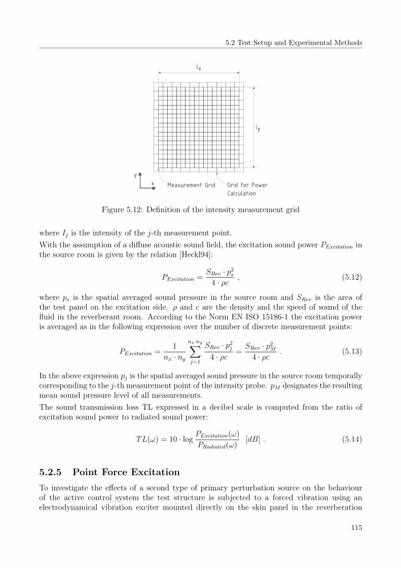
5.2 Test Setup and Experimental Methods
Measurement Grid Grid for Power
Calculation
y
x
lx
ly
Figure 5.12: Definition of the intensity measurement grid
where Ij is the intensity of the j-th measurement point.
With the assumption of a diffuse acoustic sound field, the excitation sound power PExcitation inthe source room is given by the relation [Heckl94]:
PExcitation =SRev · p2
s
4 · ρc , (5.12)
where ps is the spatial averaged sound pressure in the source room and SRev is the area ofthe test panel on the excitation side. ρ and c are the density and the speed of sound of thefluid in the reverberant room. According to the Norm EN ISO 15186-1 the excitation poweris averaged as in the following expression over the number of discrete measurement points:
PExcitation =1
nx · ny
nx·ny∑
j=1
SRev · p2j
4 · ρc =SRev · p2
M
4 · ρc . (5.13)
In the above expression pj is the spatial averaged sound pressure in the source room temporallycorresponding to the j-th measurement point of the intensity probe. pM designates the resultingmean sound pressure level of all measurements.
The sound transmission loss TL expressed in a decibel scale is computed from the ratio ofexcitation sound power to radiated sound power:
TL(ω) = 10 · logPExcitation(ω)
PRadiated(ω)[dB] . (5.14)
5.2.5 Point Force Excitation
To investigate the effects of a second type of primary perturbation source on the behaviourof the active control system the test structure is subjected to a forced vibration using anelectrodynamical vibration exciter mounted directly on the skin panel in the reverberation
115

5. Experimental Study
room as illustrated in Figure 5.10. The x- and y-positions of the shaker mounting point are233 mm and 320 mm, with x and y being the horizontal and vertical axes in the plane ofthe skin panel relative to its lower left corner. This point corresponds to an intersection of astringer-frame pair located on the other side of the skin panel. To monitor the excitation inputlevels the shaker attachment point is equipped with an additional acceleration sensor and forcetransducer.
With the transfer function g(ω) computed from the normal velocity signal x(ω) and point forceF (ω), both measured at the shaker mounting point:
g(ω) =x(ω)
F (ω)=
x(ω)
j · ω · F (ω), (5.15)
the structural excitation power can be determined as the real part of the product between forceand velocity:
PShaker(ω) = ℜ (x(ω) · F (ω)) = ℜ(g(ω) · F 2(ω)
). (5.16)
In accordance to the acoustic excitation and the norm for intensity measurement of sound TLthe mean average excitation power for nx by ny discrete measurement points is established by:
PShaker(ω) =1
nx · ny
·nx·ny∑
j=1
ℜ(gj(ω) · F 2
j (ω)), (5.17)
where gj and Fj are the transfer function and force temporally corresponding to the j-thmeasurement point of the intensity probe. The sound power radiated by the trim panel intothe anechoic chamber due to the forced vibration of the fuselage is determined by equation5.11 in the same way as for the acoustic excitation. Analogical to the transmission loss for theacoustic excitation a power ratio PR expressed in decibel can be defined for the point forceexcitation from the ratio of excitation power to radiated sound power:
PR(ω) = 10 · logPShaker(ω)
PRadiated(ω)[dB] . (5.18)
5.2.6 Measurement Implementation
The following sensor types and settings are used for the intensity and transmission loss mea-surements:
• Intensity probe: The experiments are carried out using a TFS SIP 101/SBS3i intensityprobe, which is fitted with three Sennheiser back electret condenser KE4-211-2 1/8 inchmicrophones in a side-by-side configuration. The separation distance of two microphonesis adjustable with respect to the reference microphone, thereby combining two differentmeasurement ranges into a single probe. For frequencies below 1250 Hz the microphonedistance is adjusted to 50 mm, whereas for frequencies above 1250 Hz a separation dis-tance of 8 mm is used. According to equations 5.7 and 5.9 as well as to information ofthe manufacture, the lower and upper frequency limits when allowing maximal intensitybias errors of up to 1 dB are 175 and 7800 Hz for the small microphone distance and 30and 1250 Hz for the microphone pair separated by a distance of 50 mm.
116
5.2 Test Setup and Experimental Methods
• Microphone for acoustic excitation: A half-inch pre-polarized random incidence micro-phone from G.R.A.S. Type 40 AQ mounted on a rotating transverse is used in thereverberation chamber for the determination of the excitation power.
• Point force excitation: The shaker excitation is realized with an electrodynamical vibra-tion exciter from Bruel & Kjaer Type 4809. The excitation force level is measured witha Kistler force transducer Type 9301B, whereas the structural response at the mountingpoint normal to the skin panel is monitored with a unidirectional acceleration sensor ofthe type PCB M353B65.
The output signals of the sensors are processed on an eight-channel Dolch FlexPAC systemusing the signal analyser software Ceasar µ-Remus. The analyser software also drives theintensity probe traverse mechanism so that the measurement grid is scanned automaticallyby the intensity probe. A frequency range from 0 to 1,6 kHz with a resolution bandwidthof 1 Hz is used. For both the acoustic and point force excitation the measurement data andcalculated results are available as narrowband data as well as in 1/24, 1/12, third octave andoctave bands. Further post-processing of the measurement data for the calculation of soundpower, transmission loss and intensity maps is carried out in Matlab. For the representationof intensity maps the measured data is interpolated linearly up to 400 points in the x- andy-directions and drawn on the measurement grid represented in Figure 5.12.
The excitation area SRev of the fuselage skin panel is 932 by 901 mm, which corresponds tothe inner dimensions of the clamping frame. As measurement grid, a 1 by 1 m area coveringthe trim panel with ten measurement points in the x- and y-directions is chosen. The distanceof the measurement plane to the trim panel is 300 mm. For a single point 20 individualmeasurements are averaged, requiring a time of about 20 seconds. This time is equal to theduration for a traverse period of the rotating microphone in the excitation room. The wholemeasurement procedure requires about 50 minutes.
The calibration of the intensity probe is done in two steps. First the absolute sensitivity of thereference microphone is determined with an acoustic calibrator giving a sound pressure levelof 94 dB at 1 kHz. To minimize errors in the intensity measurement, the intensity probe iscalibrated with a special piston-phone, which allows the measurement of phase and magnitudemismatches of the microphones relative to the reference microphone. These transfer functionsare then used as a correction factor when the sound intensity is calculated from the measuredcross spectral densities.
5.2.7 Measurement Repeatability
The acoustic performance evaluation of the ASAC system requires the variation in measuredtransmission loss and power ratio to be considerably smaller than the change caused by theactive system itself.
In general the following procedure is applied for the intensity measurements. The absolutesensitivity of the intensity probe is calibrated directly before each measurement. As the inten-sity analysis is very sensitive to small changes in the relative magnitude and phase mismatchof the microphones, the use of dissimilar calibration functions for the intensity probe, differingonly within the limits of measurement accuracy, could cause relatively large variations in the
117

5. Experimental Study
calculated intensity level for one and the same measurement. Hence, to exclude such effects, asingle calibration function is used when several measurements have to be compared with eachother.
To ensure the quality of the measurements with the active system the back-to-back variationof the results was investigated by repeating an intensity measurement within a period of 24hours. Figure 5.13 and 5.14 show the resulting transmission loss and power ratio curves forthese back-to-back measurements using acoustic and point force broadband excitations in thefrequency range from 0 to 1,6 kHz. The results are plotted as narrowband data using afrequency resolution of 1 Hz. As test structure, the double wall configuration with the fuselageand the first trim panel was used. The trim panel was attached to the fuselage frames via fourpassive shock mounts.
For the acoustic excitation the variations in the measurement results are considerably higherthan for the forced vibration excitation. This can be explained by the fact that for the lattercase the actual perturbation on the skin panel has a good coherence to the measured excitationpower at the shaker mounting point as no spatial averaging is required to determine the exci-tation power. In contrast to that, the acoustic excitation power is obtained from a temporallyand spatial averaged signal using the rotating microphone system in the reverberant chamber.Due to the spatial averaging the coherence between the measured sound power and the actualperturbation on the structure is not as good, resulting in a greater variation from one measure-ment to another. The frequency averaged difference between the two measurements is foundto be 0,8 dB in the frequency range from 50 to 1600 Hz for the acoustic excitation, whereasthe mean deviation in the same frequency range for the point force excitation is only 0,2 dB.Both deviations are acceptable for the evaluation of active control treatments. Nevertheless, tominimize possible errors and to guarantee the comparability of the results, the correspondingmeasurements with and without control for a specific test configuration will be carried outdirectly in succession.
As a dis- and reassembling of the test structure is not required, when carrying out the measure-ments for the different test configurations, variations due to possible changes in the installationof the test structure and the transmission loss window were not assessed.
5.3 Control Loop Implementation
A general block diagram of the control system is illustrated in Figure 5.15. The control algo-rithm is implemented in the programming language C on a laboratory dSpace DS1005 controllerboard and represents an adaptive feedforward controller. The adaptive control system is real-ized with digital filters, which are driving the secondary system paths. The filters are adjustedby an adaptive algorithm according to given reference and error signals. To ensure a goodcontroller performance, a narrowband control mode optimised for tonal primary perturbationsand a broadband mode for random primary perturbations are available. The control mode andvarious parameters are selected by the user via a real-time monitoring software installed on aseparate PC. This software is also used to monitor the DSP output and input signals as wellas the control performance and stability.
In addition to the DSP hardware, the control loop incorporates digital low-pass filters toavoid aliasing effects and high-frequency excitation of the actuators (denoted by the blocks
118

5.3 Control Loop Implementation
0 200 400 600 800 1000 1200 1400 1600−10
0
10
20
30
40
50Transmission Loss − Acoustic Excitation
Frequency [Hz]
TL
[dB
]
Measurement 1Measurement 2
Figure 5.13: Transmission loss for back-to-back measurements
0 200 400 600 800 1000 1200 1400 16000
5
10
15
20
25
30
35
Frequency [Hz]
Pow
er R
atio
[dB
]
Power Ratio − Point Force Excitation
Measurement 1Measurement 2
Figure 5.14: Power ratio for back-to-back measurements
119
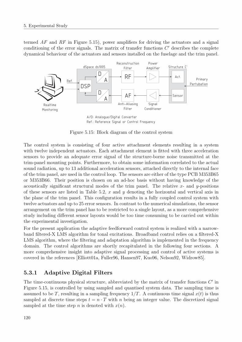
5. Experimental Study
termed AF and RF in Figure 5.15), power amplifiers for driving the actuators and a signalconditioning of the error signals. The matrix of transfer functions C ′ describes the completedynamical behaviour of the actuators and sensors installed on the fuselage and the trim panel.
dSpace ds1005
DSP
Structure C’
Sensor
AD RF
AF
Act.
Signal
Conditioner
Power
Amplifier
A/D: Analogue/Digital Converter
Ref.: Reference Signal or Control Frequency
Reconstruction
Filter
Anti-Aliasing
Filter
AD
Primary
PertubationRef.
Realtime
Monitoring
Figure 5.15: Block diagram of the control system
The control system is consisting of four active attachment elements resulting in a systemwith twelve independent actuators. Each attachment element is fitted with three accelerationsensors to provide an adequate error signal of the structure-borne noise transmitted at thetrim-panel mounting points. Furthermore, to obtain some information correlated to the actualsound radiation, up to 13 additional acceleration sensors, attached directly to the internal faceof the trim panel, are used in the control loop. The sensors are either of the type PCB M353B65or M353B66. Their position is chosen on an ad-hoc basis without having knowledge of theacoustically significant structural modes of the trim panel. The relative x- and y-positionsof these sensors are listed in Table 5.2, x and y denoting the horizontal and vertical axis inthe plane of the trim panel. This configuration results in a fully coupled control system withtwelve actuators and up to 25 error sensors. In contrast to the numerical simulations, the sensorarrangement on the trim panel has to be restricted to a single layout, as a more comprehensivestudy including different sensor layouts would be too time consuming to be carried out withinthe experimental investigation.
For the present application the adaptive feedforward control system is realized with a narrow-band filtered-X LMS algorithm for tonal excitations. Broadband control relies on a filtered-XLMS algorithm, where the filtering and adaptation algorithm is implemented in the frequencydomain. The control algorithms are shortly recapitulated in the following four sections. Amore comprehensive insight into adaptive signal processing and control of active systems iscovered in the references [Elliott01a, Fuller96, Hansen97, Kuo96, Nelson92, Widrow85].
5.3.1 Adaptive Digital Filters
The time-continuous physical structure, abbreviated by the matrix of transfer functions C ′ inFigure 5.15, is controlled by using sampled and quantised system data. The sampling time isassumed to be T , resulting in a sampling frequency 1/T . A continuous time signal x(t) is thussampled at discrete time steps t = n · T with n being an integer value. The discretized signalsampled at the time step n is denoted with x(n).
120

5.3 Control Loop Implementation
Table 5.2: Position of error sensors on the trim panel, x- and y-position [mm]
Sensor Trim Panel 1 Trim Panel 2
13 497, 790 840, 147
14 346, 645 804, 480
15 220, 535 854, 835
16 322, 330 672, 322
17 463, 185 691, 640
18 625, 329 490, 212
19 789, 481 500, 500
20 655, 620 531, 793
21 470, 487 350, 345
22 816, 286 377, 655
23 145, 810 150, 157
24 125, 294 220, 520
25 n/a 137, 834
Ref.∗ 500, 500 500, 500
∗ reference signal on fuselage skin forbroadband control
The manipulation of such signals is done with digital filters. In causal, linear systems thefilter’s output signal y(n) is affected by the current and all previous samples of the input signalx(n). Hence, the output y(n) may be written as:
y(n) =∞∑
i=0
hi · x(n− i) , (5.19)
with hi being the samples of the filter impulse response. The impulse response corresponds tothe filter output when the input is equal to the Kronecker delta function4.
A possibility to implement a digital filter in reality is to truncate the infinite summation afterI samples, thus resulting in a finite calculation time for each output sample:
y(n) =I−1∑
i=0
wi · x(n− i) . (5.20)
These filters are known as finite impulse response (FIR) filters, because the impulse responsewill be zero after I samples. By making the coefficients wi adaptive through a method thatminimises a mean square error criterion, a given input signal x(n) can be transformed intoan output y(n), representing a negative estimation of the external signal d(n). The generalstructure of such an adaptive filter element is shown on the left side of Figure 5.16.
The measured error signal e(n) can be expressed by the sum of the desired signal d(n) and thereference signal x(n) filtered by the adaptive FIR element:
e(n) = d(n) + y(n) = d(n) +I−1∑
i=0
wi(n) · x(n− i) . (5.21)
4x(n) = δ(n), which is equal to one if n = 0 and otherwise zero.
121

5. Experimental Study
Adaptive
Filter
x(n) y(n)
d(n)
e(n)
General Adaptive Digital Filter
w (n)ix(n) y(n)
d(n)
e(n)
FIR Filter adapted by LMS Algorithm
X
Figure 5.16: Adaptive digital filter and LMS adaptation
The objective of the adaptation algorithm is to determine the coefficients wi in such a way tominimise a quadratic cost function J depending on the error signal e(n):
J = E[e2(n)] → Min . (5.22)
E is an abbreviation for the expectation operator, which, for stationary signals and by assumingthat wi, i ∈ 0, . . . , I − 1 is time-invariant5, is equal to the average mean square value of theerror signal. The cost function represents a quadratic shaped surface possessing a globalminimum. The exact solution of this minimisation problem, known as the Wiener solution, isfound by differentiating J with respect to each filter coefficient and setting the derivatives tozero, ∂J/∂wi = 0.
In practice, the optimisation problem 5.22 is solved by adjusting the filter coefficients in anopposite direction proportional to the local gradient of the cost function J , thus moving theremaining error nearer towards the global minimum. The update rule for the new coefficientsmay be written as:
wi(n+ 1) = wi(n) − µ · ∂J(n)
∂wi
, (5.23)
with i ∈ 0, . . . , I − 1 and ∂J/∂wi = 2 · E[x(n − i) · e(n)]. The term µ is a convergencefactor. Instead of using this true gradient, the filter coefficients are updated every sample byan estimation of the gradient, which is equal to the derivative of the current error with respectto the filter coefficients:
∂e2(n)
∂wi
= 2 · e(n) · ∂e(n)
∂wi
= 2 · x(n− i) · e(n) . (5.24)
Thus, the adaptation rule for the filter coefficients of the next data sample becomes:
wi(n+ 1) = wi(n) − α · x(n− i) · e(n) . (5.25)
This algorithm is known as the least-mean-square (LMS) algorithm (depicted on the right sideof Figure 5.16) and converges for 0 < α < 2/(I ·x2), where x2 is the mean square value of x(n)and α = 2 · µ. For stationary signals the adaptation will automatically converge towards theoptimal Wiener filter. Advantages of the LMS algorithm are that it is simple to implement,numerical robust and represents a fast approximation to the Wiener filter problem. Besides theLMS algorithm other adaptation rules like the Newton method or the recursive least-squarealgorithm are also used for adaptive filtering operations.
5The adaptive filter varies slowly in comparison to the dynamic response of the forward path.
122

5.3 Control Loop Implementation
5.3.2 Filtered-X LMS Algorithm
Figure 5.17 shows the block diagram of an active control application where the adaptive FIRfilter is used to control the dynamic behaviour of the plant C. In this case, the filter outputcan be seen as a secondary signal (anti-noise) used to suppress a primary perturbation d(n).Since there is the dynamic system C between the filter output and the estimation of thedesired signal, the reference signal x(n) used for the filter adaptation has to be modified byan additional filter in order to ensure the stability of the controller. This particularity alsoexplains the name filtered-X LMS algorithm.
u(n) y(n)
d(n)
e(n)C
X
w (n)ix(n)
C*
r (n)*
Plant
Plant Model
Adaptive
Controller
Figure 5.17: Block diagram of the filtered-X LMS algorithm
With the assumption that the plant C may be described by an FIR filter of the order M , theerror signal is expressed as:
e(n) = d(n) + y(n) = d(n) +M−1∑
j=0
cj
I−1∑
i=0
wi(n− j) · x(n− j − i) . (5.26)
The filter is adapted in the opposite direction to the gradient of the current square error signalwith respect to the filter coefficients, which are assumed to be nearly time-invariant:
∂e2(n)
∂wi
= 2 · e(n) · ∂e(n)
∂wi
= 2 · e(n) ·M−1∑
j=0
cj · x(n− j − i) , (5.27)
where i ∈ 0, . . . , I − 1. From equation 5.27 it can be seen that, in comparison to theunmodified LMS-algorithm presented in the previous chapter, the reference signal x(n) isfiltered by the system behaviour C. Therefore, the adaptation rule for the filtered-X LMSalgorithm reads as follows:
wi(n+ 1) = wi(n) − α · r∗(n− i) · e(n) , (5.28)
with r∗(n − i) =∑M−1
j=0 c∗j · x(n − j − i) being the filtered-reference signal x(n) used for thefilter update. In practice, an estimate C∗ of the plant impulse response is used as an internalmodel for the filter operation. This plant model must include the entire dynamical behaviourbetween the output of the controller and the input, where the residual error signal is measured.Adaptive filter methods can be used to represent the real plant response. Basically, differencesbetween the estimation and the true plant response will negatively affect the stability andconvergence rate of the controller, but it has been shown in literature that the algorithm isquite robust to errors in the plant model.
123

5. Experimental Study
Since the filtered-X LMS algorithm necessitates two filter operations, the computational com-plexity is increased in comparison to the unfiltered algorithm. For this reason an efficientimplementation of the control law is required and, depending on the type of application, thealgorithm is optimised either for tonal or stochastic perturbations.
5.3.3 Multichannel Narrowband Filtered-X LMS Algorithm
It is assumed that the primary perturbation is tonal and of angular frequency ω. Control isachieved by driving the secondary control signals with the same frequency and an amplitudeand phase adjusted to minimise the perturbation. The block diagram in Figure 5.18 shows aninterpretation of the adaptive feedforward system in terms of an equivalent feedback controller.
u y
d
eCh(n)
e jwnT
C*
Plant
Plant Model
Adaptive
Controller
Figure 5.18: Block diagram of the multiple error LMS algorithm operated at the frequency ω
In the frequency domain L individual disturbance signals and M secondary control signals aredescribed by the complex vectors d(jω) and u(jω). The L×M , time-invariant plant responsesare grouped together in a complex matrix C(jω). The vector e(jω) containing the L residualerror signals can thus be written as:
e(jω) = d(jω) + C · u(jω) . (5.29)
For the prevention of large control efforts, a simple modification is made to the cost functionJ by including a component of the mean squared control signal u proportional to the positiveweighting parameter β. Hence, the cost function becomes:
J = eH(jω) · e(jω) + β · uH(jω) · u(jω) → Min , (5.30)
where eH and uH denote the Hermitian transpose of e and u. J is a quadratic function withrespect to the control signal u and thus has a minimum, which can be determined by settingthe derivative of J with respect to u to zero:
∂J
∂u= 2 · CH · e(jω) + 2 · β · u(jω) = 0 . (5.31)
The optimal control signal uopt for the steady state response is obtained as:
uopt(jω) = −(β + CH · C)−1 · CH · d(jω) . (5.32)
124

5.3 Control Loop Implementation
This optimal solution can be approximated with the filtered-X LMS algorithm. Instead of usingthe frequency transformation, the complex signals are modulated by the adaptive filter withthe term ejωnT . This modulation factor replaces the external reference signal x(n) shown inFigure 5.17 and is generated by the controller itself or synthesised from an adequate referencesignal. Hence, the resulting control signal and the adaptation rule for the update of the filtercoefficient vector h can be expressed by following two expressions:
u(n) = ℜ(h(n) · ejωnT
), (5.33)
h(n+ 1) = (1 − α · β) · h(n) − α · C∗H · e(n) · ejωnT , (5.34)
where the matrix C∗ represents an estimation of the plant impulse responses. As the controlleris reducing the primary disturbance in a narrow band around the control frequency, the algo-rithm is also known as adaptive notch filter. The bandwidth and convergence rate of controldepend directly on the parameter α. An augmentation of α will increase the bandwidth andreduce the iteration time needed to determine the optimal filter coefficients. The effort weight-ing parameter β governs the control reduction. With smaller values of β a greater reductionof the error signal will be achieved at the expense of a larger control effort [Maier00]. Thus,β always represents a compromise between optimal control performance and minimal controleffort.
Multiple tonal disturbances can be controlled by several controllers working in parallel. Ifa sufficient distance between the disturbance frequencies in comparison to the bandwidth ofcontrol is ensured, the single algorithms do barely interfere with one another.
For the current ASAC application it can be assumed that the plant response is nearly time-invariant. Therefore, prior to closing the control loop, the plant identification is made withoutexternal perturbations for every system path. This off-line system identification is realizedwith an FIR filter model, which is adapted by a filtered-X LMS algorithm using the real plantresponse as desired signal d(n).
5.3.4 Multichannel Broadband Filtered-X LMS Algorithm
The multiple error filtered-X LMS algorithm for control of broadband noise requires referencesignals having a good correlation with the original disturbance. It is assumed that a numberof K reference signals, described by the vector x(n), are available in the forward path. Forthe adaptation algorithm each reference signal is filtered by the L × M paths of the plantresponse resulting in a set of LMK filtered-reference signals for the controller update (M andL being the number of actuators and error sensors). Each FIR filter of the adaptive controlleris supposed to have I coefficients. A block diagram of the control system is shown in Figure5.19.
The output from the L error sensors is expressed in the error signal vector e(n) as superpositionfrom the primary and secondary path:
e(n) = d(n) +R(n) · w(n) , (5.35)
125

5. Experimental Study
u(n) y(n)
d(n)
e(n)Cw(n)
x(n)
C*
Matrix of Plant
Responses
Plant Model
Adaptive
Controller
X
Frequency Domain
Time Domain
Figure 5.19: Block diagram of the multichannel filtered-X LMS algorithm used for broadbandapplications
where w(n) is a vector containing the coefficients from MKI FIR filters, R(n) a L×MKImatrix containing the filtered-reference signal and d(n) a vector of L primary perturbations[Elliott01a].
The LMS algorithm will minimise a cost function J given by the sum of squared error signalsand a term proportional to the sum of squared controller coefficients. The controller coefficientsare included in the cost function to improve the controller stability with respect to inaccuraciesin the plant model C∗:
J(n) = e(n)T · e(n) + β · wT (n) · w(n) . (5.36)
β is a positive weighting parameter of the controller coefficients. The gradient vector of thecost function with respect to the filter coefficients becomes:
∂J
∂w(n)= 2 ·
(RT (n) · e(n) + β · w(n)
), (5.37)
and is used in the adaptation algorithm of the control filters, which can be expressed as:
w(n+ 1) = γ · w(n) − α ·R∗T (n) · e(n) , (5.38)
with α being the convergence rate of the filter adaptation and a leakage factor γ defined asγ = 1−α · β. The matrix R∗ contains the reference signals filtered by an estimation C∗ of thetrue plant response C.
For the present ASAC application the filtering operation of the reference signal and the filterupdate as defined in equation 5.38 are realized in the frequency domain. The adaptationalgorithm for the filter coefficients at the κ-th discrete frequency and for the m-th iterationcan be written as:
wm+1(κ) = γ · wm(κ) − α ·C∗H(κ) · em(κ) · xH
m(κ)
+, (5.39)
where the notation + indicates that for the frequency transformation of the quantitiesinside the brackets only causal parts are taken into account. The FIR control filters are stillimplemented in the time domain.
126
5.4 Experimental Results
The motivation to transfer the reference filtering and adaptation into the frequency domainis due to the fact that the computational effort is reduced in comparison to a time domainbased solution. The computational benefit can either be used to increase the number of degreesof freedom in the ASAC system or the sampling rate might be increased to control primaryperturbations at higher frequencies. Furthermore, the reaction time of the controller is reducedand it is possible to restrict control to a certain frequency range.
In the current application a single reference signal, obtained with an acceleration sensor placedat the centre of the fuselage skin, is used (referred as Ref. in Table 5.2). As both the referenceand error signals are accelerations and the radiated sound power of a vibrating structure isproportional to its squared mean velocity, both the reference and error signal are integratedwith respect to time. Thus, the weighting of the control effort at different frequencies is moreadapted to the human hearing perception and not distorted by the factor ω = 2πf with regardto the velocity.
5.4 Experimental Results
The ASAC technique with active attachment elements was tested against several acoustic andstructural perturbations. For both types of excitation various tonal and band-filtered randomsignals were used. The tonal excitation represents a temporally and spatially coherent noisesource and is similar to the buzz-saw noise excitation in real aircraft, whereas the characteristicof a random noise source, exhibiting no temporal coherence (and also no spatial coherence whenusing the acoustic excitation), resembles more to a jet noise or turbulent boundary layer noiseexcitation.
As a real excitation spectrum was not available for the experimental study, the choice of per-turbation frequencies is based upon the general transmission loss and power ratio performancemeasured with built-in active attachment elements, but with no control applied to the ASACsystem. By selecting perturbation frequencies or frequency ranges corresponding to local min-ima in transmission loss and power ratio, the worst case for sound transmission and therebyfor the acoustic passenger comfort is assumed.
Figures 5.20 and 5.21 show the resulting narrowband transmission loss and power ratio be-haviour for the acoustic and point force excitation, which were determined in preliminary testsby using a white noise excitation in the frequency band ranging from 0 to 1,6 kHz. Theseresults apply for the double wall partition in combination with the first trim panel configura-tion. In both diagrams, the black and grey curves correspond to the respective configurationswith passive shock mounts and active attachments used as connection elements between thefuselage and the trim panel.
For both types of perturbation, the different dynamic properties of the active attachmentelements and the shock mounts lead to a dissimilar sound transmission behaviour. In thefrequency ranges from 300 to 400 Hz and above 1 kHz a substantial reduction in sound trans-mission is already achieved with the active attachment elements employed in a purely passivemanner. Only around 200 Hz the performance of the system with active attachment elementsis worse than the configuration with shock mounts. At around 80 Hz the first strong couplingbetween the cavity fluid and the structure occurs and a 1,1-mode with a high radiation effi-ciency is excited on the trim panel, resulting in the global minima for transmission loss and
127

5. Experimental Study
0 200 400 600 800 1000 1200 1400 1600−10
0
10
20
30
40
50
60
Frequency [Hz]
TL
[dB
]
Transmission Loss − Acoustic Excitation
Passive Shock MountsActive Trim Panel Attachments − No Control
Figure 5.20: Transmission loss of the passive system
0 200 400 600 800 1000 1200 1400 16000
5
10
15
20
25
30
35
40
45Power Ratio − Point Force Excitation
Frequency [Hz]
Pow
er R
atio
[dB
]
Passive Shock MountsActive Trim Panel Attachments − No Control
Figure 5.21: Power ratio of the passive system
128

5.4 Experimental Results
power ratio, respectively. In this range of frequency the transmission loss values are partiallynegative, because the acoustic excitation power is underestimated by applying the diffuse fieldassumption (equations 5.12 and 5.13), which is not fulfilled at low frequencies. In the high-frequency range above 800 Hz, the passive sound reduction is higher than 30 dB and the sharpdips in the transmission loss or power ratio curves, due to a resonant sound transmission, arefar less pronounced than at lower frequencies.
5.4.1 Test Configuration
As the active technology is mainly aimed at enhancing the sound reduction in the frequencyrange up to 500 Hz, the frequencies selected for a control of tonal acoustic perturbations are78, 200, 326 and 530 Hz. Each frequency is corresponding to a local TL minima and is selectedupon the passive transmission loss behaviour in Figure 5.20. For broadband excitation withrandom noise a frequency band corresponding to the 80 Hz third octave band (ranging from71 to 90 Hz) is chosen for a first test of the broadband LMS algorithm. In a second test asimultaneous random excitation in the 80 and 200 Hz third octave band (ranging from 71 to90 Hz and 178 to 225 Hz, respectively) will be used.
The tonal perturbation frequencies for the point force excitation are 80, 199, 284 and 702 Hz,each one corresponding to a frequency with high sound transmission according to Figure 5.21.A random broadband excitation is also tested for the 80 Hz third octave band. In additionto those tests, the double wall configuration in combination with the second trim panel (seeChapter 5.2.1) is tested against an artificially generated, acoustic buzz-saw noise excitation.The fundamental frequency of this signal is 80 Hz and includes harmonics up to 3,2 kHz. Thefirst twelve frequencies will be controlled with the narrowband filtered-X LMS algorithm. Theresulting test matrix for the active structural acoustic control system is summarized in Table5.3.
Table 5.3: ASAC test matrix
Excitation Frequency Structure
Tonal acoustic: 78, 200, 326, 530 Hz Trim panel 1
Random acoustic: 80 Hz, 80 & 200 Hz third oct. band Trim panel 1
Tonal point force: 80, 199, 284, 702 Hz Trim panel 1
Random point force: 80 Hz third octave band Trim panel 1
Art. buzz-saw noise: 80 Hz and harmonics Trim panel 2
5.4.2 Results with Acoustic Excitation
The main results obtained with the ASAC control system for tonal acoustic excitations aresummarized in Table 5.4 and are given in terms of total sound power radiated by the trimpanel and mean sound pressure level in the excitation chamber for the tests with and withoutcontrol respectively. The spectral data is expressed in magnitude values using a 1 Hz frequencyresolution and the actuator voltage is defined as the ratio between the actual maximum peak
129

5. Experimental Study
actuator voltage measured during control and the absolute maximum voltage, which can beapplied to the Thunder elements (240 VPeak). Further details in terms of spectra for theradiated sound power, excitation sound pressure level and corresponding intensity plots arelisted in Annex C.
Table 5.4: Measurement results for tonal acoustic excitation
Radiated Sound Power [dB] Excitation SPL [dB] Voltage[%]Freq. control off control on control off control on
78 Hz 91,7 69,4 97,5 97,4 48,8
200 Hz 87,1 73,1 97,4 99,5 n/a
326 Hz 73,5 62,4 99,6 99,7 5,3
530 Hz 77,8 65,8 109,4 109,3 18,8
From analyzing the values given in Table 5.4, it can be seen that by controlling the dynamicbehaviour of the trim panel with the active attachment elements a substantial reduction inthe total radiated sound power can be achieved over a large band of frequencies. For exampleat 78 Hz the measured reduction in radiated sound power is 22,3 dB. At 200 Hz the soundpower attenuation is equal to 16,1 dB, whereas for 326 and 530 Hz the decrease in radiatedsound power amounts to around 11 dB. Stability problems with the control system were notencountered during the measurements and spill-over effects (unintentional excitation of higherharmonic frequencies [Fuller96, Hansen97]) did not appear with tonal primary excitations (seerespective spectra given in Annex C). The sound pressure level in the excitation room is rangingfrom around 97 dB for the 78 Hz excitation to about 109 dB at 530 Hz. The maximum actuatorworkload occurs at the first eigenfrequency of the system at 78 Hz. This eigenfrequency ischaracterized by a strong coupling between the structure and the enclosed fluid domain. Atthis frequency the tonal sound pressure level in the excitation room of around 97 dB correspondsto an actuator workload of around 50%. At higher frequencies the actuator workload is reducedto a great extent, for instance to less than 20% at 530 Hz.
To explain the general operating mode of the ASAC control system, the results achieved withthe 78 Hz tonal excitation are analyzed in more detail within the following section. The soundpressure level in the excitation room is illustrated in Figure 5.22. Rather than using a simplesinusoidal primary perturbation signal, a triangle pulse having a fundamental frequency of78 Hz is superimposed with a band-filtered white noise signal. For both measurements withand without active control a nearly identical excitation spectrum is used. The excitation soundpressure level at 78 Hz is 97 dB, whereas for the harmonics at 156, 234, 312 and 390 Hz thesound pressure levels are 105, 94, 92 and 90 dB respectively.
The ASAC narrowband control tests are carried out with a system sampling rate of 5 kHz. Thestructural response of the trim panel is controlled on the first five harmonic frequencies of thetriangle pulse with the multichannel narrowband filtered-X LMS algorithm. After identificationof the plant model C∗, various control parameter such as the convergence factor α and the effortweighting parameter β are adjusted to obtain a good control performance in combination witha reasonable control effort while maintaining the system’s stability. The input signal fromthe error sensors as well as the actuator commands are filtered by an adjustable low-pass
130

5.4 Experimental Results
50 100 150 200 250 300 350 400 45065
70
75
80
85
90
95
100
105Excitation Sound Pressure Level
Frequency [Hz]
Sou
nd P
ress
ure
Leve
l [dB
]Control offControl on
Figure 5.22: Excitation sound pressure level
filter having a cut-off frequency of 900 Hz in this case. As the filtered error signal is furthermodulated with the term ejωnT for each frequency that is controlled, a harmonic actuatorcommand is derived by the LMS algorithm. A tenth second sample of the actuator voltageis shown in Figure 5.23. The signal is dominated by the fundamental frequency of 78 Hzand the maximum voltage with a magnitude of around 117 VPeak is applied to the thirdand ninth actuator unit. On each attachment element the respective actuator units are notexcited completely in phase, indicating that combinations of both translatory and rotationaldisplacements are induced in the trim panel. This behaviour is similar to the one predictedwith the simulation model in Chapter 4.
The secondary signals induced by the actuators into the trim panel lead to a reduction ofthe vibration levels, which are measured by the respective error sensors. This relationship isillustrated in Figure 5.24, showing the time dependency of the sensor signals 6 and 21 for aperiod of five seconds and one tenth of a second with and without control respectively. Sensor6 is mounted on the second attachment element, whereas sensor 21 is located at the centre ofthe trim panel. On both sensor positions the vibration level is reduced with active control. Onsensor 21 the magnitude is decreased by more than 50%, whereas on sensor 6 mounted at oneof the trim panel attachment elements, only a small reduction is achieved.
Using all available error sensor data, the obtained overall control reduction is represented bythe two spectra plotted in Figure 5.25. The figure on the left side represents the squared sumof the twelve error signals located directly on the trim panel, whereas on the right-hand sidethe equivalent quantity for the twelve error sensors mounted on the attachment elements isreproduced. On the first four harmonics, reductions ranging between 6 and 17 dB are obtained
131

5. Experimental Study
0 0.02 0.04 0.06 0.08 0.1−150
−100
−50
0
50
100
150Attachment Element 1
Time [s]
Vol
tage
[V]
Actuator 1Actuator 2Actuator 3
0 0.02 0.04 0.06 0.08 0.1−150
−100
−50
0
50
100
150Attachment Element 2
Time [s]
Vol
tage
[V]
Actuator 4Actuator 5Actuator 6
0 0.02 0.04 0.06 0.08 0.1−150
−100
−50
0
50
100
150Attachment Element 3
Time [s]
Vol
tage
[V]
Actuator 7Actuator 8Actuator 9
0 0.02 0.04 0.06 0.08 0.1−150
−100
−50
0
50
100
150Attachment Element 4
Time [s]
Vol
tage
[V]
Actuator 10Actuator 11Actuator 12
Figure 5.23: Actuator voltage
on the trim panel sensors. At 390 Hz the error signal is only slightly decreased by 2 dB. Inthe frequency range of 220 Hz, which is not controlled, an increase of around 7 dB is noticed.This is probably due to nonlinearities in the actuator response. The general behaviour of theoverall control reduction measured on the attachment elements is similar to the one detectedon the trim panel. However, at the fundamental frequency of 78 Hz, the error level obtainedwithout control is approximately 8 dB smaller than the one on the trim panel, which is dueto the global 1,1-mode excited on the trim panel. On the remaining harmonics both vibrationlevels on the panel and on the attachment elements are of the same order of magnitude, yet theachieved control reduction on the AAE is smaller in comparison to the one on the trim paneland is ranging from 3 to around 7 dB. In the 220 Hz band the error signal is also increased.
These results demonstrate the effectiveness of the active attachment elements as structuralactuators in combination with an LMS control loop and the available sensor array. The localvibration levels measured at the sensor positions are attenuated over a large range of fre-quencies. However, the acoustic success of the control system depends furthermore on thecorrelation of the acceleration signals measured on the trim panel with the actual, radiatedsound power.
132

5.4 Experimental Results
0 1 2 3 4 5−1
−0.5
0
0.5
1Sensor 6 − Attachment Element 2
Time [s]
Acc
eler
atio
n [g
]
Control offControl on
0 1 2 3 4 5−1
−0.5
0
0.5
1Sensor 21 − Trim Panel
Time [s]
Acc
eler
atio
n [g
]
Control offControl on
0 0.02 0.04 0.06 0.08 0.1−1
−0.5
0
0.5
1Sensor 6 − Attachment Element 2
Time [s]
Acc
eler
atio
n [g
]
Control offControl on
0 0.02 0.04 0.06 0.08 0.1−1
−0.5
0
0.5
1Sensor 21 − Trim Panel
Time [s]
Acc
eler
atio
n [g
]
Control offControl on
Figure 5.24: Acceleration measured by error sensors 6 and 21, with and without control
50 100 150 200 250 300 350 400 450−45
−40
−35
−30
−25
−20
−15
−10
−5
Frequency [Hz]
Err
or S
igna
l [dB
(1g)
]
Acceleration Error Signal − Trim Panel
Control offControl on
50 100 150 200 250 300 350 400 450−45
−40
−35
−30
−25
−20
−15
−10
−5
Frequency [Hz]
Err
or S
igna
l [dB
(1g)
]
Acceleration Error Signal − AAE
Control offControl on
Figure 5.25: Squared sum of error signals on trim panel and attachment elements
133
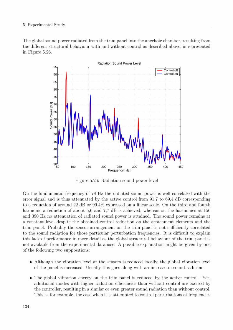
5. Experimental Study
The global sound power radiated from the trim panel into the anechoic chamber, resulting fromthe different structural behaviour with and without control as described above, is representedin Figure 5.26.
50 100 150 200 250 300 350 400 45030
35
40
45
50
55
60
65
70
75
80
85
90
95Radiation Sound Power Level
Frequency [Hz]
Sou
nd P
ower
[dB
]
Control offControl on
Figure 5.26: Radiation sound power level
On the fundamental frequency of 78 Hz the radiated sound power is well correlated with theerror signal and is thus attenuated by the active control from 91,7 to 69,4 dB correspondingto a reduction of around 22 dB or 99,4% expressed on a linear scale. On the third and fourthharmonic a reduction of about 5,6 and 7,7 dB is achieved, whereas on the harmonics at 156and 390 Hz no attenuation of radiated sound power is attained. The sound power remains ata constant level despite the obtained control reduction on the attachment elements and thetrim panel. Probably the sensor arrangement on the trim panel is not sufficiently correlatedto the sound radiation for those particular perturbation frequencies. It is difficult to explainthis lack of performance in more detail as the global structural behaviour of the trim panel isnot available from the experimental database. A possible explanation might be given by oneof the following two suppositions:
• Although the vibration level at the sensors is reduced locally, the global vibration levelof the panel is increased. Usually this goes along with an increase in sound radition.
• The global vibration energy on the trim panel is reduced by the active control. Yet,additional modes with higher radiation efficiencies than without control are excited bythe controller, resulting in a similar or even greater sound radiation than without control.This is, for example, the case when it is attempted to control perturbations at frequencies
134

5.4 Experimental Results
well below the critical frequency, which already exhibit a high passive transmission loss,as for instance at 156 Hz (TL 25,2 dB, compare with Figure 5.20) or 390 Hz (TL 31,6 dB).
Nevertheless, judging from the structural results on the sensors and the actuator effectivenessat those perturbation frequencies, it is expected that the radiation behaviour could certainlybe ameliorated by using a more appropriate sensor layout having a better correlation to thesound power radiated by the trim panel.
The sound radiation on the remaining, uncontrolled frequency bands is not affected by theactive control system, except for an increase of around 2 dB in the frequency range of 220 Hz,which was also noticed for the error signal.
The local sound intensity map for the fundamental perturbation frequency of 78 Hz is shownin Figure 5.27 for the 80 Hz third octave band with and without control. Without controla global 1,1-mode with a corresponding sound intensity pattern is excited on the trim panel.The maximum intensity is reached in the middle of the measurement grid with around 92 dB.With active control the radiation mode is still dominated by the 1,1-mode on the panel, butthe influence of higher modes in the response is increased. While controlling the structuralvibrations, the intensity is attenuated on every measurement point and the local intensitymaximum is consequently reduced to 76 dB. The mechanism associated with this type ofcontrol is active damping as the modal participation of the 1,1-mode in the structural responseto the primary perturbation is reduced for the most part.
For higher frequencies the sound radiation behaviour is more complex as, in general, besides theglobal attenuation in sound intensity, the radiation pattern is also changed due to the controlas can be seen for instance from further intensity plots listed in Annex C. This indicates thatwith the closed control loop additional modes are excited on the trim panel and the controlmechanism is also governed by a modal restructuring occurring alongside the modal dampingmechanism.
The results obtained with the control of acoustic broadband perturbations are listed in Table5.5. Numerical values are specified in the respective third octave bands. The DSP sampling rateis reduced to 1,4 kHz to take into account the increased computational costs of the broadbandfiltered-X LMS algorithm. An additional acceleration sensor, denoted as Ref. in Table 5.2,is placed on the fuselage skin and used as a reference signal for the filter adaptation. Thecontrolled frequency domain ranges from 65 to 100 Hz for the excitation in the 80 Hz thirdoctave band and from 65 to 400 Hz for the combined primary perturbations in the 80 and200 Hz band.
Table 5.5: Measurement results for random acoustic excitation
Radiated Sound Power [dB] Excitation SPL [dB] Voltage[%]Freq. control off control on control off control on
80 Hz band 86,5 76,1 100,5 100,5 55,8
80 & 200 Hz band∗ 86,1 81,1 100,0 100,1 57,4
80 & 200 Hz band∗∗ 85,0 78,0 105,2 105,3 57,4
∗ 80 Hz band results; ∗∗ 200 Hz band results
135

5. Experimental Study
70
72
74
76
78
80
82
84
86
88
90
92
x [m]
y [m
]Sound Intensity Third Octave Band 80 Hz [dB]
7071
71
71
72
72
72
72
72
73
73
73
73
73
73
73
7373
73
73
74
74
74
74
74
74
74
74
75
75
75
75
76
0 0.11 0.22 0.33 0.44 0.56 0.67 0.78 0.89 10
0.11
0.22
0.33
0.44
0.56
0.67
0.78
0.89
1
70
72
74
76
78
80
82
84
86
88
90
92
x [m]
y [m
]
Sound Intensity Third Octave Band 80 Hz [dB]
88
88
89
89
89
89
89
89
89
90
90
90
90
90 90
90
9191
91
91
91
92
92
0 0.11 0.22 0.33 0.44 0.56 0.67 0.78 0.89 10
0.11
0.22
0.33
0.44
0.56
0.67
0.78
0.89
1
Figure 5.27: Sound intensity level with (above) and without (below) ASAC control
136

5.4 Experimental Results
In contrast to the results achieved with tonal control, minor attenuations in radiated soundpower are obtained. This is mainly due to the stochastic character of the primary signal,which makes the active control more difficult. Nevertheless, for the excitation in the 80 Hzthird octave band a reduction of 10,4 dB in radiated sound power is still achieved, whereas forthe simultaneous random excitation in the 80 Hz and 200 Hz third octave band a decrease of5,1 and 7,0 dB respectively is attained. The corresponding sound pressure levels measured inthe excitation room are about 100 dB for the 80 Hz third octave band, whereas in the 200 Hzband the SPL is around 105 dB. Detailed narrowband results are also listed in Annex C.
In principle the broadband filtered-X LMS algorithm works in a similar manner as alreadyexplained for the tonal control loop. The velocity error signals are reduced in the controlledfrequency range as shown in Figure C.18 and C.19 for the combined 80 and 200 Hz bandexcitation. As the error signals have a good correlation to the radiated sound power for thecontrolled frequency range, the sound intensity in front of the trim panel is as well globallyattenuated, as indicated by the local intensity distributions shown in Figure C.16 and C.17.
Similar to the tonal excitations, the actuator voltage is dominated by the system response inthe 80 Hz third octave band. In this case a relative actuator workload of 56% (80 Hz thirdoctave band excitation) and 58% (simultaneous 80 and 200 Hz third octave band excitation)is resulting. An exemplary sample of the actuator excitation is given in Figure C.20 for thesimultaneous excitation in both frequency bands. The actuators of each attachment elementare driven mainly in phase, which is also noticed for the 80 Hz third octave band excitation.At those specific frequencies and probably without an important loss in performance, thecontrol system could also be operated with simplified attachment elements, generating onlypure translatory displacements. However, this would also limit the control performance athigher perturbation frequencies.
Typical for broadband control is the fact that energy is shifted to frequency bands havinga lower energy content within the controlled frequency range. In particular this so-calledwaterbed effect is observed for the random excitation in the 80 and 200 Hz third octave band(see Figure C.14), where the sound radiation is increased in the 315 Hz third octave band anda reduction is achieved in the 400 Hz band. In both test cases increased sound radiation isalso noticed in uncontrolled frequency bands. For instance, while controlling the excitation inthe 80 Hz third octave band, sound power is amplified in the 200 Hz third octave band from29 to 38 dB and in the 250 Hz band from 24 to 47 dB (Figure C.11). This effect has not beeninvestigated in detail but may be explained by nonlinearities of the actuators. Anyway, thelevels are still well below the mean sound power level of 76,1 dB measured in the controlled80 Hz band. For the configuration with a combined 80 and 200 Hz third octave band excitationthis effect is less distinctive, but still present. An increase in sound radiation from 22 to 32 dBcan be observed with the closed control loop in the 500 Hz band, compared to levels in thecontrolled 80 and 200 Hz third octave bands of 81,1 dB and 78,0 dB respectively.
5.4.3 Results with Point Force Excitation
The general results obtained with the ASAC control of point force perturbations are listed inTable 5.6 and 5.7. The values are given in terms of total radiated sound power and excitationforce for the tests with and without control. For the tonal excitations the results are given
137
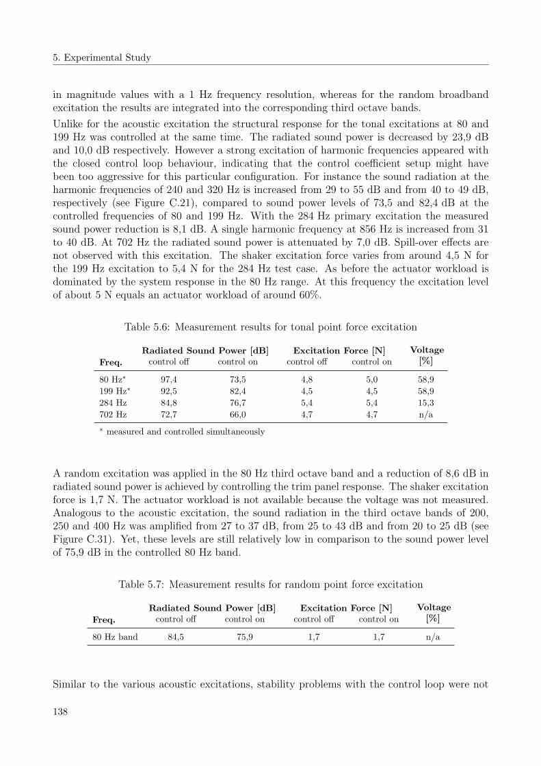
5. Experimental Study
in magnitude values with a 1 Hz frequency resolution, whereas for the random broadbandexcitation the results are integrated into the corresponding third octave bands.
Unlike for the acoustic excitation the structural response for the tonal excitations at 80 and199 Hz was controlled at the same time. The radiated sound power is decreased by 23,9 dBand 10,0 dB respectively. However a strong excitation of harmonic frequencies appeared withthe closed control loop behaviour, indicating that the control coefficient setup might havebeen too aggressive for this particular configuration. For instance the sound radiation at theharmonic frequencies of 240 and 320 Hz is increased from 29 to 55 dB and from 40 to 49 dB,respectively (see Figure C.21), compared to sound power levels of 73,5 and 82,4 dB at thecontrolled frequencies of 80 and 199 Hz. With the 284 Hz primary excitation the measuredsound power reduction is 8,1 dB. A single harmonic frequency at 856 Hz is increased from 31to 40 dB. At 702 Hz the radiated sound power is attenuated by 7,0 dB. Spill-over effects arenot observed with this excitation. The shaker excitation force varies from around 4,5 N forthe 199 Hz excitation to 5,4 N for the 284 Hz test case. As before the actuator workload isdominated by the system response in the 80 Hz range. At this frequency the excitation levelof about 5 N equals an actuator workload of around 60%.
Table 5.6: Measurement results for tonal point force excitation
Radiated Sound Power [dB] Excitation Force [N] Voltage[%]Freq. control off control on control off control on
80 Hz∗ 97,4 73,5 4,8 5,0 58,9
199 Hz∗ 92,5 82,4 4,5 4,5 58,9
284 Hz 84,8 76,7 5,4 5,4 15,3
702 Hz 72,7 66,0 4,7 4,7 n/a
∗ measured and controlled simultaneously
A random excitation was applied in the 80 Hz third octave band and a reduction of 8,6 dB inradiated sound power is achieved by controlling the trim panel response. The shaker excitationforce is 1,7 N. The actuator workload is not available because the voltage was not measured.Analogous to the acoustic excitation, the sound radiation in the third octave bands of 200,250 and 400 Hz was amplified from 27 to 37 dB, from 25 to 43 dB and from 20 to 25 dB (seeFigure C.31). Yet, these levels are still relatively low in comparison to the sound power levelof 75,9 dB in the controlled 80 Hz band.
Table 5.7: Measurement results for random point force excitation
Radiated Sound Power [dB] Excitation Force [N] Voltage[%]Freq. control off control on control off control on
80 Hz band 84,5 75,9 1,7 1,7 n/a
Similar to the various acoustic excitations, stability problems with the control loop were not
138

5.4 Experimental Results
observed. Further details in terms of spectra for the radiated sound power, excitation soundpressure level and corresponding intensity plots are listed in Annex C.
5.4.4 Results with Artificial Buzz-Saw Noise Excitation
The experimental results presented in the previous chapters were achieved with a relativelycomplex control system based on a fully coupled interaction between 12 actuators and 24 or25 acceleration error sensors respectively. A possible application and integration into a realaircraft cabin would certainly be easier for a less complex system. This could either be achievedby reducing the number of actuators or error sensors involved in the control loop. However, theresults achieved so far also revealed that, mainly for excitation frequencies higher than 200 Hz,the actuators of an attachment element are always driven to some extent out of phase, implyingthat a combination of both translatory and rotational displacements is induced by the DSPsystem at the trim panel attachment points and thus required for a good control performance.Reducing the number of degrees of freedom by driving the respective three actuators of eachattachment element in phase (hence simulating a system with four degrees of freedom instead oftwelve) would thus limit the control authority to excitation frequencies under 200 Hz. For thisreason and as a typical buzz-saw noise excitation also involves higher perturbation frequencies,it was decided to test the ASAC control system with a reduced number of error sensors inorder to assess the potentials of a system with decreased control complexity.
As a test case for this experimental investigation an artificial buzz-saw noise excitation is used.According to the buzz-saw noise data given in Chapter 2 the fundamental frequency is chosento equal 80 Hz. The excitation signal contains 40 harmonics up to 3,2 kHz and is shaped togive a similar radiation spectrum as the one presented in Figure 2.6. In contrast to the othertests a second trim panel had to be used, denoted as Trim Panel 2 in Table 5.3. The reductionin the number of error sensors is achieved by using only sensors placed directly on the trimpanel. The remaining sensors on the attachment elements are not used in the control loop,but are still available to measure the respective acceleration levels with and without control.In total 13 sensors are used. Their respective position on the trim panel is listed in Table 5.3.
The first twelve perturbation frequencies up to 960 Hz are controlled with the narrowbandfiltered-X LMS algorithm, using the same controller parameters as for the previous tonaltests (sample rate 5 kHz, low-pass filter with cut-off frequency set to 1,1 kHz). The mainresults are summarized in Annex C, Figure C.34 and C.35 for the global radiated sound powerand excitation sound pressure level. The following reductions on the controlled harmonicfrequencies, starting with 80 Hz, are obtained in radiated sound power by controlling the localdynamic trim panel response at the sensor positions: 5, 12, 6, 2, 0, 4, 2, 5, 9, 1, 0 and 2 dB. Theoverall reduction, integrated from 0 to 1,6 kHz, is dominated by the peak at 240 Hz and equals6,2 dB or about 76% on a linear scale. It should be noted that for instance the excitationsat 400 and 560 Hz coincide with local high transmission loss values, which makes the activecontrol more difficult. Presumably, the global attenuations could be further improved by usingdifferent sensor arrangements, optimised in regard to their correlation to the radiated soundpower.
Samples of the acceleration signals measured with sensor 6 (on the second attachment element2 and not controlled) and sensor 21 (trim panel) are presented in Figure C.36. On the trimpanel a substantial reduction is achieved, whereas on the attachment element only a slight
139
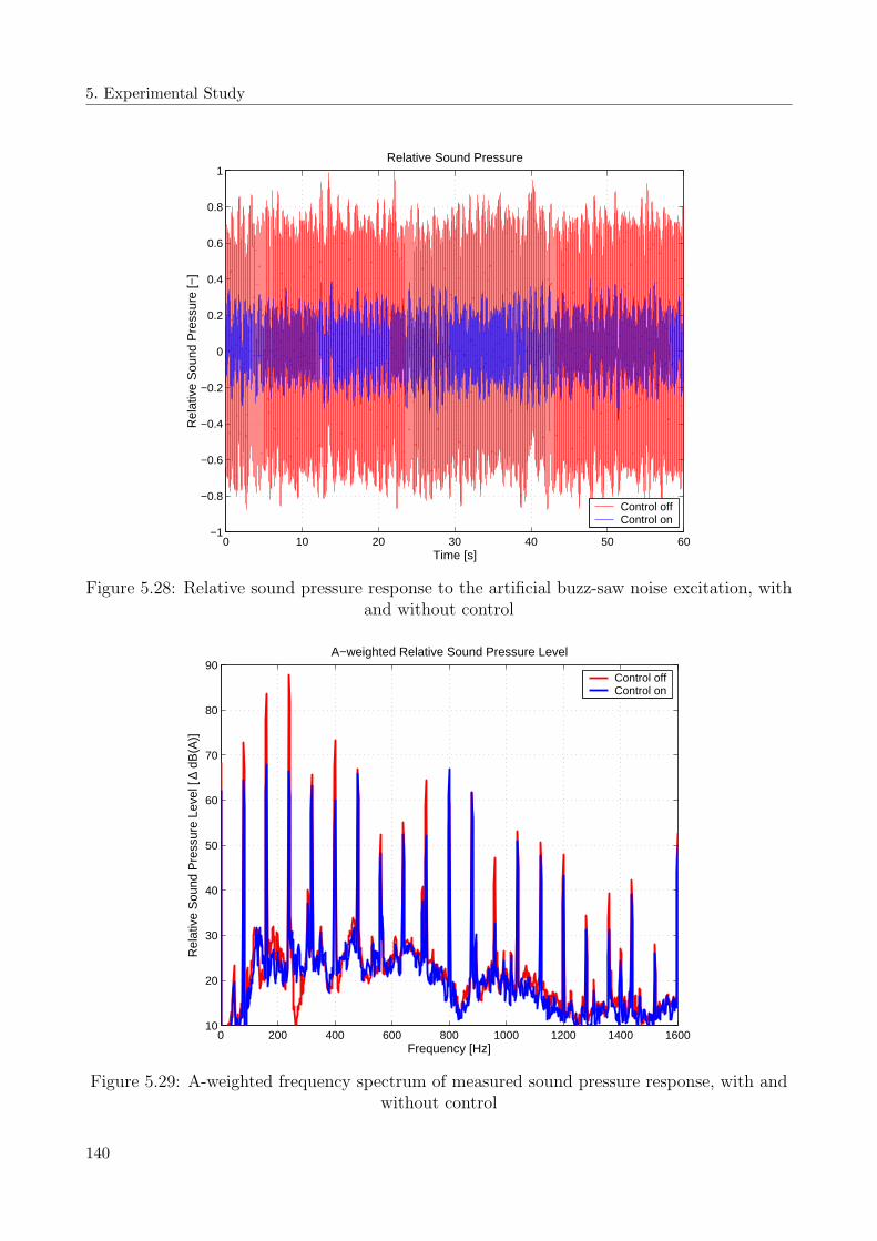
5. Experimental Study
0 10 20 30 40 50 60−1
−0.8
−0.6
−0.4
−0.2
0
0.2
0.4
0.6
0.8
1Relative Sound Pressure
Time [s]
Rel
ativ
e S
ound
Pre
ssur
e [−
]
Control offControl on
Figure 5.28: Relative sound pressure response to the artificial buzz-saw noise excitation, withand without control
0 200 400 600 800 1000 1200 1400 160010
20
30
40
50
60
70
80
90A−weighted Relative Sound Pressure Level
Frequency [Hz]
Rel
ativ
e S
ound
Pre
ssur
e Le
vel [
∆ d
B(A
)]
Control offControl on
Figure 5.29: A-weighted frequency spectrum of measured sound pressure response, with andwithout control
140
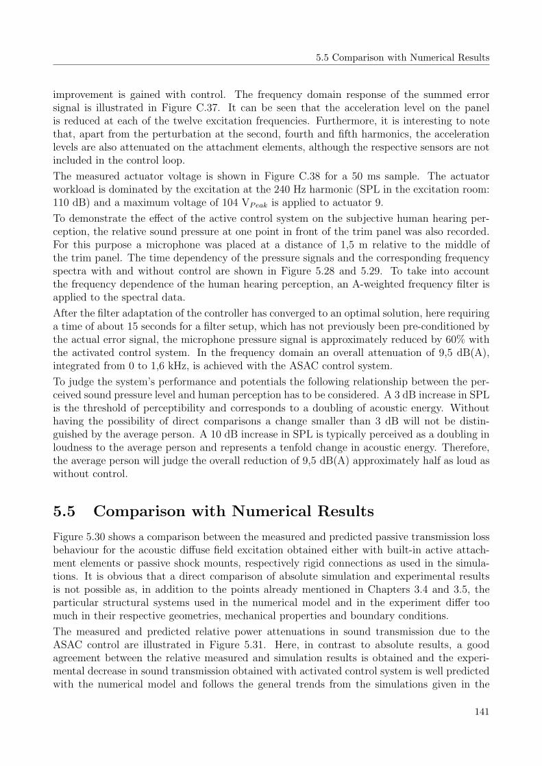
5.5 Comparison with Numerical Results
improvement is gained with control. The frequency domain response of the summed errorsignal is illustrated in Figure C.37. It can be seen that the acceleration level on the panelis reduced at each of the twelve excitation frequencies. Furthermore, it is interesting to notethat, apart from the perturbation at the second, fourth and fifth harmonics, the accelerationlevels are also attenuated on the attachment elements, although the respective sensors are notincluded in the control loop.
The measured actuator voltage is shown in Figure C.38 for a 50 ms sample. The actuatorworkload is dominated by the excitation at the 240 Hz harmonic (SPL in the excitation room:110 dB) and a maximum voltage of 104 VPeak is applied to actuator 9.
To demonstrate the effect of the active control system on the subjective human hearing per-ception, the relative sound pressure at one point in front of the trim panel was also recorded.For this purpose a microphone was placed at a distance of 1,5 m relative to the middle ofthe trim panel. The time dependency of the pressure signals and the corresponding frequencyspectra with and without control are shown in Figure 5.28 and 5.29. To take into accountthe frequency dependence of the human hearing perception, an A-weighted frequency filter isapplied to the spectral data.
After the filter adaptation of the controller has converged to an optimal solution, here requiringa time of about 15 seconds for a filter setup, which has not previously been pre-conditioned bythe actual error signal, the microphone pressure signal is approximately reduced by 60% withthe activated control system. In the frequency domain an overall attenuation of 9,5 dB(A),integrated from 0 to 1,6 kHz, is achieved with the ASAC control system.
To judge the system’s performance and potentials the following relationship between the per-ceived sound pressure level and human perception has to be considered. A 3 dB increase in SPLis the threshold of perceptibility and corresponds to a doubling of acoustic energy. Withouthaving the possibility of direct comparisons a change smaller than 3 dB will not be distin-guished by the average person. A 10 dB increase in SPL is typically perceived as a doubling inloudness to the average person and represents a tenfold change in acoustic energy. Therefore,the average person will judge the overall reduction of 9,5 dB(A) approximately half as loud aswithout control.
5.5 Comparison with Numerical Results
Figure 5.30 shows a comparison between the measured and predicted passive transmission lossbehaviour for the acoustic diffuse field excitation obtained either with built-in active attach-ment elements or passive shock mounts, respectively rigid connections as used in the simula-tions. It is obvious that a direct comparison of absolute simulation and experimental resultsis not possible as, in addition to the points already mentioned in Chapters 3.4 and 3.5, theparticular structural systems used in the numerical model and in the experiment differ toomuch in their respective geometries, mechanical properties and boundary conditions.
The measured and predicted relative power attenuations in sound transmission due to theASAC control are illustrated in Figure 5.31. Here, in contrast to absolute results, a goodagreement between the relative measured and simulation results is obtained and the experi-mental decrease in sound transmission obtained with activated control system is well predictedwith the numerical model and follows the general trends from the simulations given in the
141
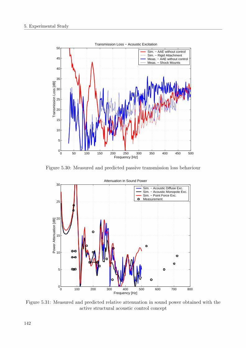
5. Experimental Study
0 50 100 150 200 250 300 350 400 450 5000
5
10
15
20
25
30
35
40
45
50Transmission Loss − Acoustic Excitation
Frequency [Hz]
Tra
nsm
issi
on L
oss
[dB
]Sim. − AAE without controlSim. − Rigid AttachmentMeas. − AAE without controlMeas. − Shock Mounts
Figure 5.30: Measured and predicted passive transmission loss behaviour
0 100 200 300 400 500 600 700 8000
5
10
15
20
25
30
Frequency [Hz]
Pow
er A
ttenu
atio
n [d
B]
Attenuation in Sound Power
Sim. − Acoustic Diffuse Exc.Sim. − Acoustic Monopole Exc.Sim. − Point Force Exc.Measurement
Figure 5.31: Measured and predicted relative attenuation in sound power obtained with theactive structural acoustic control concept
142
5.6 Conclusions
previous chapter. Furthermore, the results confirm that with the active attachment elements asufficient control authority is guaranteed for a large band of frequencies and even at relativelyhigh frequencies, as for instance at 720 Hz, a good performance can be attained, despite usinga single, non-optimised sensor configuration on the trim panel. Also, the measured actuatorvoltage lies within the limits given by the simulation model. This proves that reliable sim-ulation results can be obtained for relatively complex systems such as the considered doublewall structure, which allows the transmission of sound by airborne and structure-borne pathsand has an incorporated active control system. Thus, the use of adequate numerical modelsenables and facilitates the development and design process of ASAC systems.
5.6 Conclusions
A prototype of an active system to reduce the low-frequency sound transmission through air-craft sidewall structures was developed and tested on a representative generic aircraft structureinstalled in an acoustic test facility between a reverberant sending room and anechoic receivingroom.
The control system consists of active trim panel attachment elements replacing the existingpassive shock mounts. The actuator design is based on commercially available piezoelectricbending elements and the unique design of the elements enables the excitation of both trans-latory and rotational perturbations on each attachment point, thus permitting an efficientstructural acoustic control of the trim panel. The controller is either implemented in a multi-channel narrowband or broadband filtered-X LMS configuration on a laboratory DSP systemand uses structural accelerations as an error signal. The functionality and performance of thewhole system was successfully demonstrated with various tonal and broadband disturbancesat different frequencies. Either loudspeaker or shaker point force excitations of realistic levelswere used as primary perturbation source.
The experimental results prove that the sound radiation from lightweight structures such astrim panels can be substantially reduced by means of a structural acoustic control conceptbased on active trim panel attachment elements. The best experimental results were achievedin the low-frequency range where typical aircraft sidewalls are less efficient in reducing thesound transmission into the cabin. Reductions in radiated sound power in the order of 20 dBand more were obtained with active control in contrast to the uncontrolled configuration. Withincreasing frequencies the dynamic behaviour of the trim panel is more and more dominatedby higher modes and therefore more difficult to control with a limited number of actuatorsand sensors. Nevertheless, even at tonal perturbations of 530 and 702 Hz, reductions of 11 and7 dB in sound power were obtained with the prototype control system. The sound intensitymeasurements show that the sound field radiated by the trim panel is spatially evenly reducedin magnitude with active control, indicating that a reduction of structural vibration energy isthe main mechanism underlying the active control concept.
Mechanical problems with the actuators as well as stability problems within the control loopwere not encountered during the experiments. As expected, the critical case for the actuatordesign turns out to be the first eigenfrequency of the system, where a strong coupling betweenthe structure and the enclosed cavity occurs, resulting in the maximum structural displace-ments and thus requiring the most important actuation effort. Considerably lower actuator
143

5. Experimental Study
voltages are needed for controlling higher frequency disturbances.
In contrast to the simulations, only a single sensor configuration was tested in the main investi-gations. However, further testing with a second available trim panel was possible and an activecontrol system with a reduced number of error sensors also improved the sound transmissionbehaviour by a considerable amount for a hypothetical buzz-saw noise excitation. Based on thetwo items, experimental and simulation results, it is therefore presumed that the active systemcould be further optimised in terms of acoustic gains and system complexity by using errorsignals having a better correlation to the actual excitation and sound radiation behaviour.
A direct comparison of absolute simulation and experimental results is not possible, as therespective structural systems differ too much in geometry and mechanical properties. However,the relative experimental results obtained with and without control match the general trendsfrom the simulation predictions given in the previous chapter. The increase in TL is wellpredicted with the numerical model and also the measured actuator voltage lies within thelimits given by the simulation model. This proves that, even for a relative complex systemas the considered double wall structure with fluid-structure coupling and incorporated activecontrol loop, reliable results can be obtained with an adequate numerical model.
144
Chapter 6
Summary and Recommendations
Current commercial aircraft have the least capacity in reducing structural sound transmissionat low frequencies and it is expected that, with the development and introduction of compositefuselage structures in future aircraft, the low-frequency transmission loss behaviour will be-come even worse. Hence, for the preservation and further improvement of acoustical passengercomfort at low audible frequencies, appropriate noise control methods are required. Yet, dueto mass and volume requirements in aircraft design, the successful use of conventional noisecontrol technologies (acoustic insulation, constrained layer damping, etc.) is limited in thelower frequency range. An alternative noise control solution, requiring less additional weightand volume, is provided with the concept of active structural acoustic control. ASAC systemsare based on the principle that by controlling the vibration response of a structure with appro-priate actuators and sensors, its structural sound radiation can be reduced. Subsequently, thedevelopment and testing of a prototype ASAC system, intended to increase the low-frequencytransmission loss of aircraft sidewalls by controlling its structural response, has been addressedin this thesis.
In a first step the conception and basic design of such a control concept has been investigatedwith a numerical, modular simulation model. The simulation methodology is based on anFEM-description of the structure since with this approach relatively complex structures canbe taken into account (for instance, double wall partitions with fluid-structure coupling, soundtransmission by airborne and structure-borne paths, stiffened structures and complex mate-rials). Assuming a weak coupling to the surrounding fluid, the resulting sound radiation ismodelled with the Huygens-Rayleigh integral by post-processing the vibration results obtainedfor a given excitation on the radiating surface. The vibro-acoustic simulation model was val-idated with a series of transmission loss experiments carried out on a single and double wallaluminium partition. A good agreement between the predicted and measured sound transmis-sion behaviour has been found and the simulation method has been proved to be an efficienttool for TL calculations.
Active elements, such as piezoelectric patches bonded to the structure, are described within theFEM-model by simplified actuation laws such as the thermal-elastic analogy or the equivalentforce model. These actuation models provide a linear relationship between the applied voltageand the actuation forces introduced into the substrate structure and are considered to besufficiently accurate since only the general impact of the control input on the global structuralresponse has to be determined. A simplified control loop is incorporated in the computation

6. Summary and Recommendations
model by applying the superposition principle. By minimising an error signal, the requiredactuation signal is derived and, based on the assumption of a linear structural behaviour,the controlled structural response can be computed as a linear combination of the structuralresponse due to the primary perturbation and the secondary, controller-generated responses.Thus, the system response represents an estimate of the best possible controller performance fora given system configuration and can be compared to the uncontrolled response or alternativecontrol systems in terms of structural and sound radiation behaviour.
The numerical model has been used to determine an appropriate active control system in-tended to reduce the low-frequency sound transmission through typical aircraft sidewalls. Thebasic structural model consists of a simplified, flat aluminium fuselage structure stiffened byperpendicular stringers and frames in conjunction with a generic honeycomb core trim panel.Sound transmission is dominated by the cavity fluid path but also possible through the trimpanel attachments that mechanically couple the fuselage behaviour to the trim panel. Threedifferent ASAC systems have been evaluated against several primary excitations applied tothe fuselage skin (acoustic monopole field, diffuse field and point force excitation). Two ofthe active systems are based on piezoceramic patches either bonded directly to the fuselageskin or the trim panel. As control law, a local velocity feedback control loop in conjunctionwith collocated sensors was used in both cases, thus increasing the structural damping andenergy dissipation in the sound transmission path. A new ASAC concept was devised with thethird concept. The system consists of active attachment elements that are mounted betweenthe fuselage and the trim panel and replace the conventional trim panel mounts. The activeattachment element is designed to provide three independent degrees of freedom, allowing thecontrol of both normal translatory and rotational perturbation components induced on the trimpanel at the attachment points. Actuation is done by piezoceramic elements. The controllerwas implemented in an LMS-configuration and combined with acceleration sensors located onthe trim panel and the attachment elements.
Out of the three investigated systems, the best low-frequency control performance in termsof radiated sound power and structural vibration reduction was obtained with the active at-tachment elements. An added advantage of such a system in comparison to the other controltechnologies is that for a sidewall system, where sound transmission is dominated by structure-borne components, the active attachments elements also represent the most adequate controlsolution.
To demonstrate the efficiency of such a system, further work was directed on the developmentand experimental testing of a prototype control system based on active attachment elements.For the actuation, commercially available piezo actuators have been used. The prototype activeattachment element has a weight of just 100 g and dimensions of 23 mm in height and of 62 mmin diameter. A plane aircraft sidewall section (dimensions 1 by 1 m), consisting of a genericCFRP fuselage and a honeycomb core trim panel, was fitted with four prototype attachmentelements and subsequently installed in a transmission loss test suite between a reverberationand an anechoic chamber. The LMS controller was implemented on a laboratory DSP systemand consisted of 12 control channels combined with a total of up to 26 acceleration error signals.Excitation was carried out in the reverberation chamber on the fuselage skin, either acousticallyby loudspeakers or mechanically by a point force excitation. In the anechoic chamber, facingthe trim panel, the transmitted sound power was determined by intensity measurements. Theperformance and efficiency of the active system was evaluated against several deterministic and
146
random disturbances, representing noise sources similar to buzz-saw noise, jet noise and TBLnoise excitations. The disturbance frequencies were chosen according to the sound transmissionbehaviour measured without control and correspond to local frequencies where the sidewallstructure has the least efficiency in reducing the sound transmission. Realistic excitation levelshave been used.
From the experimental results one can conclude that the active attachment elements representan efficient technology for the active control of sound transmission through aircraft sidewallstructures and thus provide new possibilities to attenuate low-frequency disturbances in thecabin and improve passenger comfort. The effect of control has been clearly audible and sub-stantial decreases in sound transmission have been obtained for a large band of frequencies.Best results were achieved at low frequencies, as for instance on the mass-air-mass resonance,where tonal reductions in radiated sound power in the order of 20 dB or even more wereobtained. Control authority is reduced with increasing frequency but even at relatively highfrequencies good attenuations in radiated sound power can be attained. For non-deterministicperturbations third octave band reductions of up to 10 dB have been measured with the pro-totype system. The main mechanism of control is a reduction of the overall kinetic trim panelenergy, which is linked to a spatial evenly attenuation in the magnitude of the sound intensityradiated by the trim panel.
Problems with the control system and the actuators were not encountered throughout thedifferent test configurations. In all cases the control loop remained stable during the durationof each individual intensity measurement, which typically required a time of around 50 minutes.In terms of actuator performance, the critical frequency was the mass-air-mass resonance ofthe system, requiring the highest actuation efforts due to the large displacements excited onthe trim panel. At higher frequencies the actuators were driven well below their maximumoperating voltage. Furthermore, the control concept with active attachment elements providessome advantages compared to other technologies like active noise control with loudspeakers,active damping of the main structure or active panels with structurally integrated actuators.Active attachment elements allow an easy retrofitting and maintenance, they are fail-safe, theacoustic performance is easily scalable according to the primary excitation and the elementscan be designed to improve the transmission loss by means of passive and active vibrationisolation.
Yet, further work is needed to optimise the presented ASAC concept with respect to a successfulcommercial application. The most important point concerns the array of error sensors used onthe trim panel. In the experimental investigations only one particular sensor layout, chosen onan ad-hoc basis without having knowledge of the exact radiation modes of the trim panel, wasused. The particular sensor array was probably sub-optimally placed, an effect having a greaterinfluence at higher perturbation frequencies. Therefore, no reduction in sound power wasobtained with control on some frequencies, even though the vibration levels on the error sensorsin the feedback loop were reduced. This indicates that in these configurations acoustically non-relevant vibrations were controlled. It is believed that better results in terms of sound powerreduction can be obtained if suitable error sensors correlated to the actual sound radiation areused. Furthermore, some experimental results confirmed that the active control system is alsoable to work with a reduced number of error sensors. In addition to that, a reduction in thenumber of control channels could be possible for the lowest perturbation frequency such as themass-air-mass resonance. This would reduce the complexity of the control system, but is also
147

6. Summary and Recommendations
dependant on the actual structural boundary conditions.
Another point concerns directly the design of the active attachment elements. For future ap-plications the performance, weight and volume of the actuators can be further optimised. Inthe current application, for instance, it would be possible to integrate the aluminium mountingplates directly into the trim panel and the frames respectively. Consequently, with a struc-turally integrated design the required installation height could be reduced from around 23 to11 mm. Furthermore, the basic clamshell units also have a potential for further miniaturisingand, by redesigning the structural attachment to the individual Thunder elements, actuatorperformance could be improved as well.
Finally, the electronic hardware components used in the laboratory test have a high weightand require a large volume. With respect to one of the main objectives typically claimedfor active control systems, which is the reduction of weight and volume in comparison toconventional passive noise control methods, this may be seen as problematic by potentialcustomers. For a successful demonstration of an integral ASAC system in aircraft and fora possible commercial application, it is therefore strongly recommended to miniaturise theelectronic hardware components such as the DSP system, power amplifiers, filters and signalconditioners.
148

Bibliography
Achkire, Y. (1997). Active Tendon Control of Cable-Stayed Bridges. Active Structures Labo-ratory, Universite Libre de Bruxelles, Belgium.
Bao, C. and J. Pan (1997). Experimental study of different approaches for active control ofsound transmission through double walls. Journal of Acoustical Society of America, 102(3),pp. 1664-1670.
Barisciano, L.P. (1999). Broadband Transmission Loss Due to Reverberant Excitation.NASA/CR-1999-209687, Langley Research Center.
Bathe, K.-J. (1982). Finite Element Procedures in Engineering Analysis. Prentice-Hall, Inc.,Englewood Cliffs, New Jersey.
Baumann, W.T., F.-S. Ho, and H.H. Robertshaw (1992). Active structural acoustic controlof broadband disturbances. Journal of Acoustical Society of America, 92(4), pp. 1998-2005.
Bebesel, M. (1999). Aktive Schwingungsdampfung zur Larmminderung in Fahrzeugkabinen.Physik-Departement Institut E15, Technische Universitat Munchen.
Beranek, L.L. and G.A. Work (1949). Sound Transmission through Multiple Structures Con-taining Flexible Blankets. Journal of Acoustical Society of America, 21(4), pp. 419-428.
Berry, A., J.L. Guyader, and J. Nicolas (1990). A general formulation for the sound radia-tion from rectangular, baffled plates with arbitrary boundary conditions. Journal of AcousticalSociety of America, 88(6), pp. 2792-2802.
Bianchi, E., P. Gardonio, and S.J. Elliott (2004). Smart panel with multiple decentralizedunits for the control of sound transmission. Part III: control system implementation. Journalof Sound and Vibration, 274, pp. 215-232.
Blakely, K. (1993). MSC/Nastran - Basic Dynamic Analysis, Version 68. MacNeal-Schwendler Corporation.
Bliss, D.B. (1982). Study of bulk reacting porous sound absorbers and a new boundary condi-tion for thin porous layers. Journal of Acoustical Society of America, 71(3), pp. 533-545.
Bliss, D.B. and S.E. Burke (1982). Experimental investigation of the bulk reaction boundarycondition. Journal of Acoustical Society of America, 71(3), pp. 546-551.
Bossens, F. (2001). Amortissement actif des structures cablees: de la theorie al’implementation. Active Structures Laboratory, Universite Libre de Bruxelles, Belgium.

Bibliography
Braunling, W. (2004). Flugzeugtriebwerke - Grundlagen, Aero-Thermodynamik, Kreispro-zesse, Thermische Turbomaschinen, Komponenten und Emissionen. Springer-Verlag, Berlin,Heidelberg, New York.
Burdisso, R.A., J.S. Vippermann, and C.R. Fuller (1993). Causality analysis of feedforward-controlled systems with broadband inputs. Journal of Acoustical Society of America, 94(1), pp.234-242.
Bushnell, G.S., T.M. Anderson, M.D. Becraft, and A. Dean Jacot (1997). Active rackisolation system development for the international space station. AIAA-97-1203, 38thAIAA/ASME/AHS/ASC Structures, Structural Dynamics and Material Conference, Kissim-mee, USA.
Cabos, C. and F. Ihlenburg (2003). Vibrational Analysis of Ships with Coupled Finite andBoundary Elements. Journal of Computational Acoustics, Vol. 11, No. 1, pp. 91-114.
Cady, W.G. (1964). Piezoelectricity 2: An introduction to the theory and applications ofelectromechanical phenomena in crystals. Dover Publications, New York.
Carneal, P.J. and C.R. Fuller (1993). Active Structural Acoustic Control of Noise Trans-mission through Double Panel Systems. AIAA-93-4421, 15th Aeroacoustics Conference, LongBeach.
Carneal, P.J. and C.R. Fuller (2003). An analytical and experimental investigation of activestructural acoustic control of noise transmission through double panel systems. Journal ofSound and Vibration, 272, pp. 749-771.
Carneal, J.P., F. Charette, and C.R. Fuller (2004). Minimization of sound radiation fromplates using adaptive tuned vibration absorbers. Journal of Sound and Vibration, 270, pp.781-792.
Cazzolato, B.S. and C.H. Hansen (2000). Errors in the measurement of acoustic energydensity in one-dimensional sound fields. Journal of Sound and vibration, 256(5), pp. 801-831.
Charette, F., C.R. Fuller, and J.P. Carneal (1997). Adaptive vibration absorbers for controlof sound radiation from panels. AIAA-97-1619, 3rd AIAA/CEAS Aeroacoustics Conference1997, Atlanta, USA.
Charette, F., A. Berry, and C. Guigou (1997). Radiation modes and the active control ofsound power. Journal of Acoustical Society of America, 103(3), pp. 1493-1503.
Chen, Y., X.G. Wang, C. Sun, F. Devine, and C.W. de Silva (2003). Active Vibration Controlwith State Feedback in Woodcutting. Journal of Vibration and Control, 9, pp. 645-664.
Clark, R.L. and C.R. Fuller (1992). Experiments on active control of structurally radiatedsound using multiple piezoceramic actuators. Journal of Acoustical Society of America, 91(6),pp. 3313-3320.
150

Bibliography
Clark, R.L. and C.R. Fuller (1992). Modal sensing of efficient acoustic radiators withpolyvinylidene fluoride distributed sensors in active structural acoustic control. Journal ofAcoustical Society of America, 91(6), pp. 3321-3329.
Clark, R.L. and C.R. Fuller (1992). Optimal placement of piezoelectric actuators and po-livinylidene fluoride error sensors in active structural control approaches. Journal of Acous-tical Society of America, 92(3), pp. 1521-1533.
Coanda, H. (1930). Procede de protection contre les bruits. French Patent FR 722.274. Filed:Oct. 21, 1930. Patented: Dec. 29, 1931.
Coanda, H. (1932). Procede et dispositif de protection contre les bruits. French Patent FR762.121. Filed: Dec. 31, 1932. Patented: Jan. 18, 1934.
Collins, S.G. and A.H. von Flotow (1991). Active vibration for spacecraft. IAF-91-289, 42ndCongress of the International Astronautical Federation, Montreal, Canada.
Cook, R.D., D.S. Malkus, and M.E. Plesha (1989). Concepts and Applications of Finite Ele-ment Analysis. Springer-Verlag, Berlin, Heidelberg.
Conover, W.B. and W.F.M. Gray (1955). Noise Reducing System for Transformers. U.S.Patent US 2,776,020. Filed: Feb. 9, 1955. Patented: Jan. 1, 1957.
Corcos, G.M. (1963). Resolution of Pressure in Turbulence. Journal of Acoustical Society ofAmerica, 35(2), pp. 192-199.
Cremer, L. and M. Heckl (1996). Korperschall - Physikalische Grundlagen und technischeAnwendung. Springer-Verlag, Berlin, Heidelberg.
Crighton, D.G., A.P Dowling, J.E. Ffowcs Williams, M. Heckl, and F.G. Leppington (1992).Modern methods in analytical acoustics: lecture notes. Springer-Verlag, Berlin HeidelbergNew York.
Crocker, M.J. (1998). Measurement of Sound Intensity. In Harris, C.M.: Handbook of Acous-tical Measurements and Noise Control, Acoustical Society of America.
De Fonseca, P., P. Sas, and H. Van Brussel (1998). Active control of sound transmis-sion through an aircraft fuselage test section. AIAA-98-2233, Proceedings of the FourthAIAA/CEAS Aeroacoustics Conference 1998, Toulouse, pp. 184-194.
De Fonseca, P., P. Sas, and H. Van Brussel (1999). Experimental Study of the Active SoundTransmission Reduction Through a Double Panel Test Section. Acustica & Acta Acustica,Vol. 85, pp. 538-546.
De Man, P., A. Francois, and A. Preumont (2003). Active control of noise transmissionthrough double wall structures. An overview of possible approaches. NCTAM-2003-099, 6thNational Congress on Theoretical and Applied Mechanics, Ghent, Belgium.
Denkena, B., A. Harms, and P. Hesse (2004). Adaptronischer Werkzeugadapter zur aktivenSchwingungsdampfung in CNC-Drehmaschinen. Adaptronic Congress 2004.
151

Bibliography
Elliott, S.J. and M.E. Johnson (1993). Radiation modes and the active control of sound power.Journal of Acoustical Society of America, 94(4), pp. 2194-2204.
Elliott, S. (2001). Signal Processing for Active Control. Academic Press Limited, London.
Elliott, S.J. and P. Gardonio (2001). Active Control of Sound Transmission. Internoise 2001,The Hague, Netherlands.
Estorff, O. von (2000). Boundary elements in acoustics: advances & applications. WIT Press,Southampton, UK.
Fahy, F.J. (1977). Measurement of acoustic intensity using cross-spectral density of two mi-crophone signals. Journal of Acoustical Society of America, 62(4), pp. 1057-1059.
Fahy, F.J. (1985). Sound and Structural Vibration: Radiation, Transmission and Response.Academic Press Limited, London.
Fahy, F.J. (1989). Sound Intensity. Elsevier Applied Sciences, New York.
Franchek, M.A., R.J. Bernhard, and M. Ryan (1993). Adaptive/passive noise and vibrationcontrol. AIAA-93-1147, AIAA/AHS/ASEE Aerospace Design Conference 1993, Irvine, USA.
Fuller, C.R. and R.J. Silcox (1992). Active structural acoustic control. Journal of AcousticalSociety of America, 91(1), pp. 519.
Fuller, C.R., S.J. Elliot, and P.A. Nelson (1996). Active Control of Vibration. Academic PressLimited, London.
Gardonio, P. and S.J. Elliott (1998). Active control of structure-borne and airborne soundtransmission through a double panel. AIAA-98-2353, Proceedings of the Fourth AIAA/CEASAeroacoustics Conference 1998, Toulouse, pp. 864-879.
Gardonio, P., Y.-S. Lee, S.J. Elliott, and S. Debost (2001). Analysis and measurement ofa matched volume velocity sensor and uniform force actuator for active structural acousticcontrol. Journal of Acoustical Society of America, 110(6), pp. 3025-3031.
Gardonio, P. and S.J. Elliott (2004). Smart panel for active structural acoustic control.Journal of Smart Materials and Structures, 13, pp. 1314-1336.
Gardonio, P., E. Bianchi, and S.J. Elliott (2004). Smart panel with multiple decentralizedunits for the control of sound transmission. Part I: theoretical predictions. Journal of Soundand Vibration, 274, pp. 163-192.
Gardonio, P., E. Bianchi, and S.J. Elliott (2004). Smart panel with multiple decentralizedunits for the control of sound transmission. Part II: design of the decentralized control units.Journal of Sound and Vibration, 274, pp. 193-213.
Graham, W.R. (1995). The influence of curvature on the sound radiated by vibrating panels.Journal of Acoustical Society of America, 71(3), pp. 533-545.
152
Bibliography
Groeneweg, J.F., G. Sofrin, E.J. Rice, and P.R. Gliebe (1995). Turbomachinery Noise. InHubbard, H.: Aeroacoustics of Flight Vehicles: Theory and Practice - Volume 1: NoiseSources, pp. 151-209, Acoustical Society of America, Woodbury.
Grosveld, F.W. (1996). Numerical Comparison of Active Acoustic and Structural Noise Con-trol in Stiffened Double Wall Cylinder. American Institute of Aeronautics and Astronautics.
Guicking, D. (2003). From a Laboratory Curiosity to Commercial Products. Drittes Physika-lisches Institut, University of Gottingen.
Guy, R.W. and P. Sauer (1984). The influence of sills and reveals on sound transmission loss.Journal of Applied Acoustics, 17, pp. 453-476.
Halliwell, R.E. and A.C. Warnock (1985). Sound transmission loss: Comparison of conven-tional techniques with sound intensity techniques. Journal of Acoustical Society of America,77, pp. 2094-2103.
Hansen, C.H. and S.D. Snyder (1997). Active Control of Noise and Vibration . E. & F.N.Spon, London.
Heckl, M. and H.A. Muller (1994). Taschenbuch der technischen Akustik. Springer-Verlag,Berlin, Heidelberg.
Henderson, T.C. (1996). Design and testing of a broadband active vibration isolation systemusing stiff actuators. Proceedings of the Annual AAS Rocky Mountain Guidance and ControlConference 1999, Breckenridge, USA.
Henrioulle, K. and P. Sas (2001). A PVDF sensor/actuator pair for active control of soundtransmission. Internoise 2001, The Hague, Netherlands.
Henrioulle, K. and P. Sas (2003). Experimental validation of a collocated PVDF volume ve-locity sensor/actuator pair. Journal of Sound and vibration, 265(3), pp. 489-506.
Hyde, T.T. (1997). An experimental study of active vibration isolation. AIAA-97-1354,38th AIAA/ASME/AHS/ASC Structures, Structural Dynamics and Material Conference,Kissimmee, USA.
Ingard, K.U. (1994). Notes on Sound Absorption Technology. Noise Control Foundation, Ar-lington Branch, Poughkeepsie.
Jacobsen, F. (2002). A note on finite difference estimation of acoustic particle velocity. Jour-nal of Sound and Vibration, 256(5), pp. 849-859.
Jakob, A. (1999). Aktive Minderung der Schallabstrahlung schwingender Platten. Fortschritt-Berichte VDI, Reihe 11, Nr. 280, Dusseldorf.
Janocha, H. (1992). Aktoren - Grundlagen und Anwendung. Springer-Verlag, Berlin, Heidel-berg.
Johnson, M.E. and S.J. Elliott (1995). Active control of sound radiation using volume velocitycancellation. Journal of Acoustical Society of America, 98(4), pp. 2174-2186.
153

Bibliography
Jones, R.E. (1979). Intercomparison of laboratory determinations of airborne sound transmis-sion loss. Journal of Acoustical Society of America, 66(1), pp. 148-164.
Kihlman, T. and A.C. Nilsson (1972). The effects of some laboratory designs and mountingcondition on reduction index measurements. Journal of Sound and Vibration, 24, pp. 349-364.
Kim, B.-K., H.-J. Kang, J.-S. Kim, H.-S. Kim, and S.-R. Kim (2004). Tunnelling effect insound transmission loss determination: Theoretical approach. Journal of Acoustical Societyof America, 115(5), pp. 2100-2109.
Kropp, A. and D. Heiserer (2003). Efficient Broadband Vibro-Acoustic Analysis of PassengerCar Bodies using an FE-based Component Mode Synthesis Approach. Journal of Computa-tional Acoustics, Vol. 11, No. 2, pp. 139-157.
Kubo, Y. (2004). Prospects for the Suppression of Aerodynamic Vibrations of a Long-SpanBridge Using Boundary-Layer Control. Journal of Vibration and Control, 10, pp. 1359-1373.
Kuo, S.M. and D.R. Morgan (1996). Active Noise Control Systems - Algorithms and DSPImplementations. John Wiley & Sons, Inc., New York.
Lago, T.L. (2002). Industry Overview of Active Control Methods and Applications. Adaptro-nic Congress 2002.
Lammering, R. and S. Wiesemann (1998). Numerical and Experimental Investigations onSmart Structures with Piezoelectric Devices. In Gabbert, U.: Modelling and Control of Adap-tive Mechanical Structures, Fortschritt-Berichte VDI, Reihe 11, Nr. 268, Dusseldorf.
Lee, C.K. (1990). Theory of laminated piezoelectric plates for the design of distributed sen-sors/actuators. Part I: Governing equations and reciprocal relationships. Journal of AcousticalSociety of America, 87(3), pp. 1144-1158.
Lee, C.K., W.W. Chiang, and T.C. O’Sullivan (1991). Piezoelectric modal sensor/actuatorpairs for critical active damping vibration control. Journal of Acoustical Society of America,90(1), pp. 374-384.
Lee, Y.-S., P. Gardonio, and S.J. Elliott (2002). Volume velocity vibration control of a smartpanel using a uniform force actuator and an accelerometer array. Journal of Smart Materialsand Structures, 11, pp. 863-873.
Lewy, S. (2000). Experimental study of fan broadband noise on a turbofan model. 7th Inter-national Congress on Sound and Vibration, Garmisch-Partenkirchen.
Li, Q.S., D.K. Liu, J. Tang, N. Zhang, and C.M. Tam (2004). Combinatorial optimal designof number and positions of actuator in actively controlled structures using genetic algorithms.Journal of Sound and Vibration, 270, pp. 611-624.
Lilley, G.M. (1995). Jet Noise - Classical Theory and Experiments. In Hubbard, H.: Aeroa-coustics of Flight Vehicles: Theory and Practice - Volume 1: Noise Sources, pp. 211-289,Acoustical Society of America, Woodbury.
154
Bibliography
Locatelli, G. (2001). Piezo-actuated adaptive structures for vibration damping and shapecontrol - modelling and testing. Fortschritt-Berichte VDI, Reihe 11, Nr. 303, Dusseldorf.
Lorkowski, T. (2001). Piezoelektrische Hybridaktuatoren fur eine dynamische Profilvariati-on als Hochauftriebshilfe an Helikopterrotoren. Fortschritt-Berichte VDI, Reihe 12, Nr. 451,Dusseldorf.
Lueg, P. (1933). Verfahren zur Dampfung von Schallschwingungen. Austrian Patent No.141998. Filed: Feb. 2, 1933. Patented: Jan. 15, 1935.
Maier, R. (2000). Innenlarmminderung bei Helikoptern durch aktive Korperschallisolation. InAutomatisierungstechnik 48, Oldenbourg Verlag, pp. 191-198.
Maier, R., F. Hoffmann, S. Tewes, and M. Bebesel (2002). Active Vibration Isolation Systemfor Helicopter Interior Noise Reduction. AIAA 2002-2495, 8th AIAA/CEAS AeroacousticConference, Breckenridge.
Maillard, J.P. and C.R. Fuller (1994). Advanced time domain wave-number sensing for struc-tural acoustic systems. I. Theory and design. Journal of Acoustical Society of America, 95(6),pp. 3252-3261.
Maillard, J.P. and C.R. Fuller (1994). Advanced time domain wave-number sensing for struc-tural acoustic systems. I. Active radiation control of a simply supported beam. Journal ofAcoustical Society of America, 95(6), pp. 3262-3272.
Maillard, J.P. and C.R. Fuller (1995). Advanced time domain wave-number sensing for struc-tural acoustic systems. I. Experiments on active broadband radiation control of a simply sup-ported plate. Journal of Acoustical Society of America, 98(5), pp. 2613-2621.
Maillard, J.P. and C.R. Fuller (1997). Comparison of two structural sensing approaches foractive structural acoustic control. Journal of Acoustical Society of America, 103(1), pp. 396-400.
Mangiante, G.A. (1977). Active sound absorption. Journal of Acoustical Society of America,61(6), pp. 1516-1523.
Marburg, S. and H.-J. Hardtke (2003). Investigation and Optimization of a Spare Wheel Wellto Reduce Vehicle Interior Noise. Journal of Computational Acoustics, Vol. 11, No. 3, pp.425-449.
Masson, P., A. Berry, and J. Nicolas (1997). Active structural acoustic control using strainsensing. Journal of Acoustical Society of America, 102(3), pp. 1588-1599.
Maury, C., P. Gardonio, and S.J. Elliott (2001). Model for Active Control of Flow-InducedNoise Transmitted through Double Partitions. AIAA-2001-2111, AIAA/CEAS 7th Aeroacous-tics Conference, Maastricht, Netherlands.
May, D.N., K.J. Plotkin, R.G. Selden, and B.H. Sharp (1985). Lightweight Sidewalls forAircraft Interior Noise Control. NASA/CR-172490, McDonnell Douglas Corporation, DouglasAircraft Company, Long Beach.
155

Bibliography
McAlpine, A. and M.J. Fisher (2001). On the prediction of buzz-saw noise in aero-enginesinlet ducts. Journal of Sound and Vibration, 248, pp. 123-149.
McKenna, J.T. (1993). Airline Outlook: Silencing Saab 340s. Aviation Week & Space Tech-nology, February 1, pp. 17.
Mechel, F.P. (2002). Formulas of Acoustics. Springer-Verlag, Berlin, Heidelberg, New York.
Mixson, J.S. and J.F. Wilby (1995). Interior Noise. In Hubbard, H.: Aeroacoustics of FlightVehicles: Theory and Practice - Volume 2: Noise Control, pp. 271-355, Acoustical Society ofAmerica, Woodbury.
Moosrainer, M. (2000). Fluid-Struktur-Kopplung. Vibroakustische Losungsmethoden und An-wendungen. Fortschritt-Berichte VDI, Reihe 11, Nr. 289, Dusseldorf.
Morse, P.M. and K. Uno Ingard (1986). Theoretical Acoustics. Princeton University Press,Princeton, USA.
Nelson, P.A. and S.J. Elliott (1992). Active Control of Sound. Academic Press Limited, Lon-don.
Nijhuis, M.O. (2003). Analysis Tools for the Design of Active Structural Acoustic ControlSystems. Ponsen & Looijen bv., Wageningen, Netherlands.
Olson, H.F. and E.G. May (1953). Electronic Sound Absorber. Journal of Acoustical Societyof America, 25(6), pp. 1130-1137.
Olson, H.F. (1953). Electronic Sound Absorber. U.S. Patent US 2,983,790. Filed: April 30,1953. Patented: May 9, 1961.
Olson, H.F. (1956). Electronic Control of Noise, Vibration, and Reverberation. Journal ofAcoustical Society of America, 28(5), pp. 966-972.
Padula, S.L. and R.K. Kincaid (1999). Optimization Strategies for Sensor and ActuatorPlacement. NASA/TM-1999-209126.
Palumbo, D.L., R. Cabell, J. Cline, and B. Sullivan (1999). Flight Test of ASAC AircraftInterior Noise Control System. AIAA-99-1933.
Palumbo, D., R. Cabell, J. Cline, and B. Sullivan (2000). Active Structural Acoustic Controlof Interior Noise on a Raytheon 1900D. NASA/TM-2000-209846.
Pan, J. and C.H. Hansen (1990). Active control of noise transmission through a panel into acavity. I: Analytical study. Journal of Acoustical Society of America, 87(5), pp. 2098-2108.
Pan, J. and C.H. Hansen (1991). Active control of noise transmission through a panel into acavity. II: Experimental study. Journal of Acoustical Society of America, 90(3), pp. 1488-1492.
Pan, J. and C.H. Hansen (1991). Active control of noise transmission through a panel intoa cavity. III: Effect of the actuator location. Journal of Acoustical Society of America, 90(3),pp. 1493-1501.
156
Bibliography
Pan, J. and C. Bao (1998). Analytical study of different approaches for active control ofsound transmission through double walls. Journal of Acoustical Society of America, 103(4),pp. 1916-1922.
Pan, X., J. Sutton, and S.J. Elliott (1998). Active control of sound transmission through adouble-leaf partition by volume velocity cancellation. Journal of Acoustical Society of America,104(5), pp. 2828-2835.
Papadopoulos, C.I. (2003). Development of an optimised, standard procedure to calculatesound transmission loss: numerical results. Journal of Applied Acoustics, 64 (2003), pp.1069-1085.
Parkins, J.W., S.D. Sommerfeldt, and J. Tichy (2000). Error analysis of a practical energydensity sensor. Journal of Acoustical Society of America, 108(1), pp. 211-222.
Peiffer, A., S. Bruhl, C. Moeser, and S. Tewes (2005). Zeitoptimierte Berechnung des Schall-durchgangs durch Wandstrukturen mittels FEM. DAGA 2005, Munchen.
Preumont, A. (1997). Vibration Control of Active Structures. Kluwer Academic Publishers,Dordrecht.
Rafaely, B., S.J. Elliott, and J. Garcia-Bonito (1999). Broadband performance of an activeheadrest. Journal of Acoustical Society of America, 106(2), pp. 787-793.
Rapp, H. (1996). Faserverbundwerkstoffe und Piezokeramiken - eine Materialkombinationmit Zukunft. In Faserverbundstrukturen und -bauweisen in der Luft- und Raumfahrt, DGLR-Tagung, Ottobrunn.
Rohwer, K. (1996). Modelle und Methoden zur Berechnung von Laminaten aus unidirektio-nalen Faserverbunden. Fortschritt-Berichte VDI, Reihe 01, Nr. 264, Dusseldorf.
Rosen, C.Z. and B.V. Hiremath (1992). Piezoelectricity. AIP American Institute of Physics,New York.
Schmidt, H. (1996). Schalltechnisches Taschenbuch: Schwingungskompendium. VDI-Verlag,Dusseldorf.
Sessler, G.M. (1981). Piezoelectricity in polyvinylidenefluoride. Journal of Acoustical Societyof America, 70(6), pp. 1596-1608.
Skudrzyk, E. (1971). The Foundations of Acoustics. Springer-Verlag, Wien.
Sollo, A., L. Lecce, V. Quaranta, and N. Doelman (1998). Active noise control on ATRfuselage mock-up by piezoceramic actuators. AIAA-98-2230, Proceedings of the FourthAIAA/CEAS Aeroacoustics Conference 1998, Toulouse, pp. 174-183.
Swanson, D.A. and L.R. Miller (1993). Design and Effectiveness Evaluation of an ActiveVibration Isolation System for a Commercial Jet Aircraft. AIAA-93-1145, AIAA/AHS/ASEEAerospace Design Conference, Irvine, CA, USA.
157

Bibliography
Thayer, D., M. Campbell, and J. Vagners (1999). Six axis vibration isolation using moderncontrol techniques. Proceedings of the Annual AAS Rocky Mountain Guidance and ControlConference 1999, Breckenridge, USA.
Thomas, D.R. and P.A. Nelson (1995). Feedback control of sound radiation from a plateexcited by a turbulent boundary layer. Journal of Acoustical Society of America, 98(5), pp.2651-2662.
Thomas, R., M. Choudhari, and R. Joslin (2002). Flow and Noise Control: Review andAssessment of Future Directions. NASA/TM-2002-211631, Langley Research Center.
Tran, B.N., G.P. Mathur, and P.G. Bremner (1995). Modal energy analysis of aircraft sidewallresponse to acoustic fields. Internoise 95, Newport Beach, CA, USA.
Tsai, S.W. and H. Hahn (1980). Introduction to Composite Materials. Technomic Publ. Co.,Westport, USA.
Ungar, E.E., J.F. Wilby, D.B. Bliss, B. Pinkel, and A. Galaitsis (1977). A Guide for Estima-tion of Aeroacoustic Loads on Flight Vehicle Surfaces - Volume 1. AFFDL-TR-76-91-Vol.1,U.S. Air Force.
Wallace, C.E. (1972). Radiation Resistance of a Rectangular Panel. Journal of AcousticalSociety of America, 51(3), pp. 946-952.
Wang, B.T., C.R. Fuller, and E.K. Dimitriadis (1991). Active control of noise transmissionthrough rectangular plates using multiple piezoelectric or point force actuators. Journal ofAcoustical Society of America, 90(5), pp. 2820-2830.
Warnock, A.C. (1982). The influence of specimen frame on sound transmission loss measure-ments. Journal of Applied Acoustics, 15, pp. 307-314.
Widrow, B. and S.D. Stearns (1985). Adaptive Signal Processing. Prentice-Hall, Inc., Engle-wood Cliffs, New Jersey.
Wilby, J.F. and T.D. Scharton (1973). Acoustic transmission through a fuselage sidewall.NASA/CR-132602, Bolt Beranek and Newman Inc., Cambridge, MA, USA.
Williams, E.G. (1997). On Green’s function for a cylindrical cavity. Journal of AcousticalSociety of America, 102(6), pp. 3300-3307.
Witting, M. (1999). Modelling of Diffuse Sound Field Excitations and Dynamic ResponseAnalysis of Lightweight Structures. Herbert Utz Verlag, Munchen.
Wright, R.I. and M.R.F. Kidner (2004). Vibration Absorbers: A Review of Applications inInterior Noise Control of Propeller Aircraft. Journal of Vibration and Control, 10, pp. 1221-1237.
158

Appendix A
Modelling of Piezoelectric Actuators
A.1 Mechanical Behaviour of Laminate Plates with Ac-
tive Elements
Considering a small element of a multi-layer laminate plate with integrated piezoceramicpatches as illustrated in Figure 3.7, the force induced by the actuators into the substratelayers can be calculated by using the classical laminate theory [Locatelli01, Rohwer96, Tsai80].This approach expands the following analysis to plates made of orthotropic laminate layers.For a single orthotropic laminate layer the constitutive material equations for plane stress andlinear elasticity are described by:
σ1
σ2
τ12
=
Q11 Q12 0Q12 Q22 00 0 Q66
·
ǫ1ǫ2γ12
−
0 0 d31
0 0 d31
0 d15 0
·
U1/t1U2/t2U3/t3
⇔ (σ) = [Q] ·(ǫ− Λ
). (A.1)
The subscript 1 denotes the local principal material direction (for instance the fibre orientation)and 2 its transversal direction. The vector Λ contains the free piezoelectric strain that isinduced in the actuator layers with the assumption of a uniform electric field Ui/ti. Thepiezoelectric characteristics in 1- and 2-direction are similar, d32 = d31. For a passive laminatelayer Λ has to be set to zero. Q is the reduced stiffness matrix of the orthotropic layer and itselements Qij are given by1:
Q11 =E1
1 − ν12ν21
, Q12 =ν12 · E2
1 − ν12ν21
,
Q22 =E2
1 − ν12ν21
, Q66 = G12 . (A.2)
1For a unidirectional composite layer the material parameters in the local principle directions can be calcu-lated from the fibre and matrix properties [Rohwer96, Tsai80].

A. Modelling of Piezoelectric Actuators
With the known principal orientation ϕk of each layer k defined relative to the x-axis of theglobal x,y,z-coordinate system, the reduced stiffness matrix Q is transformed into the globalcoordinate system.
Qk = T−1σ ·Qk ·
(T−1
σ
)T, (A.3)
where Tσ is the stiffness transformation matrix as defined by the following expression:
Tσ =
cos2 ϕk sin2 ϕk 2 · sinϕk · cosϕk
sin2 ϕk cos2 ϕk −2 · sinϕk · cosϕk
− sinϕk · cosϕk sinϕk · cosϕk cos2 ϕk − sin2 ϕk
. (A.4)
It follows from the assumption of the Kirchhoff hypothesis2 that the strain field is linear throughthe thickness direction of the plate. This also implies a perfect bonding for each layer. Thestrain in the plate can then be written as:
ǫxǫyγxy
=
ǫ0xǫ0yγ0
xy
+ z ·
κx
κy
κxy
. (A.5)
The vector ǫ0 is denoting the deformation of the reference plane and κ its curvature. They aredefined as:
ǫ0xǫ0yγ0
xy
=
∂u0/∂x∂v0/∂y
∂u0/∂y + ∂v0/∂x
,
κx
κy
κxy
= −
∂2w0/∂x2
∂2w0/∂y2
2 · ∂2w0/∂x∂y
, (A.6)
where u0, v0 and w0 are the displacements of the structure in x-, y- and z-direction respectively.
Introducing expressions A.3 and A.5 into equation A.1 leads to the stress-strain equation fora single layer expressed in the global coordinate system.
σx
σy
τxy
=
Q11 Q12 Q12
Q12 Q22 Q26
Q16 Q26 Q66
·
ǫxǫyγxy
−
0 0 d31
0 0 d31
0 d15 0
·
U1/t1U2/t2U3/t3
⇔ (σ) =[Q
]·((ǫ0 + z · κ
)− Λ
). (A.7)
By integrating the stresses in expression A.7 over the thickness t of the laminate the externalforces are obtained:
2A section perpendicular to the undeformed mid-plane remains straight and perpendicular to the deformedmid-plane.
160

A.2 Actuator Force Models
Nx
Ny
Nxy
=
∫
t
σx
σy
τxy
· dz =
N∑
k=1
∫ zk
zk−1
σx
σy
τxy
k
· dz =
=
∫
tot
[Q
]·(ǫ0 + z · κ
)· dz −
∫
act
[Q
]· Λ · dz ,
Mx
My
Mxy
=
∫
t
σx
σy
τxy
· z · dz =
N∑
k=1
∫ zk
zk−1
σx
σy
τxy
k
· z · dz =
=
∫
tot
[Q
]·(ǫ0 + z · κ
)· z · dz −
∫
act
[Q
]· Λ · z · dz , (A.8)
where zk is the z-coordinate of the surface between the layers k and k + 1 with respect to thereference plane. The subscripts tot and act refer, respectively, to an integration over the wholestructure incorporating the passive laminate layers as well as the actuator layer, and over theactuator layer only. In matrix form equation A.8 can be rewritten as:
(NM
)=
[A BB D
]
tot
·(ǫ0
κ
)−
[AB
]
act
· Λ . (A.9)
The abbreviations A, B and D denote the usual stiffness matrices used in the classical laminatetheory. Its elements ij are given by:
Matrix of in-plane stiffness: Aij =N∑
k=1
Qij,k · (zk − zk−1) ,
Matrix of coupling stiffness: Bij =1
2·
N∑
k=1
Qij,k ·(z2
k − z2k−1
),
Matrix of rotational stiffness: Dij =1
3·
N∑
k=1
Qij,k ·(z3
k − z3k−1
). (A.10)
The in-plane stiffness matrix A connects the in-plane deformation ǫ0 to the in-plane forces,the matrix D of rotational stiffness relates the curvature κ with the moments, whereas thecoupling stiffness matrix B associates in-plane deformations with moments and curvature within-plane forces. For a symmetrical laminate lay-up the coupling matrix B is zero.
A.2 Actuator Force Models
In order to determine the forces induced by the actuator patches into the structure, the externalforces in equation A.9 are set to zero and the equivalent deformations ǫ0 and κ, induced intothe structure when applying an electric field Λ to the actuators, are obtained:
161

A. Modelling of Piezoelectric Actuators
(ǫ0
κ
)
eq
=
[A BB D
]−1
tot
·[AB
]
act
· Λ . (A.11)
Replacing the deformations in equation A.9 (without taking into account the free piezoelectricstrain Λ) with those obtained from equation A.11 results in the equivalent external forces thathave to be applied along the edges of the piezo patch in the selected reference plane to givethe same strain distribution as by excitation of the actuators:
(NM
)
eq
=
[A BB D
]
tot
·(ǫ0
κ
)
eq
=
[AB
]
act
· Λ . (A.12)
If the reference plane is chosen to be located in the mid-plane of the actuator, the couplingmatrix Bact is zero due to the symmetry. Applying an electric field in 3-direction will result ina force of N = Aact · Λ. The amount of this force is equal to the blocked force of the actuator,hence this model is also referred to as blocked force model.
If the mass and stiffness added by an active element is small in comparison to the substratelayers, the global behaviour of the laminate plate may be analysed without considering thepiezoelectric material. In this case the integration in equation A.12 has to be made over thethickness of the laminate plate only and the equivalent forces are defined by:
(NM
)
eq
=
[A BB D
]
hs
·(ǫ0
κ
)
eq
=
[A BB D
]
hs
[A BB D
]−1
tot
·[AB
]
act
· Λ . (A.13)
The subscript hs refers to an integration over the host structure. For a static analysis thismodel will give the same results in terms of global structural deformation as the blockedforce model represented by equation A.12. However, in a dynamic analysis, the influenceof the added actuator mass and stiffness on the eigenfrequencies and mode shapes of theplate is not taken into account. Nevertheless, it has been shown that this method provides agood approximation to analyse the transversal dynamic behaviour of plates fitted with smallpiezoceramic d31-patches [Bebesel99, Lammering98, Locatelli01, Nijhuis03].
In addition expression A.13 can be used to optimise the actuator thickness with respect toa given laminate lay-up and material parameters. A common application is the bimorpharrangement with surface-bonded piezo patches located on one side of the laminate plate. Withincreasing actuator thickness the in-plane forces will augment, whereas the bending moments,introduced into the structure by an excitation of the actuators, will exhibit a maximum for acertain piezoceramic thickness.
This relation is illustrated in the following figure where the equivalent forces are plotted asfunctions of the actuator thickness for a 2 mm steel and aluminium plate used as substratelayer (material properties are listed in Table A.1). It is assumed that a constant electric field of-1000 V/mm, regardless of the actuator thickness, is applied in 3-direction. As reference plane,the symmetry plane of the substrate layer is chosen. Due to the isotropic material behaviourthe in-plane forces in x- and y-direction are of the same magnitude.
For an optimal coupling of the bending moments into the structure the actuator thicknesswould have to be 1,7 mm for the steel plate and 1,1 mm for the less stiff aluminium plate.
162
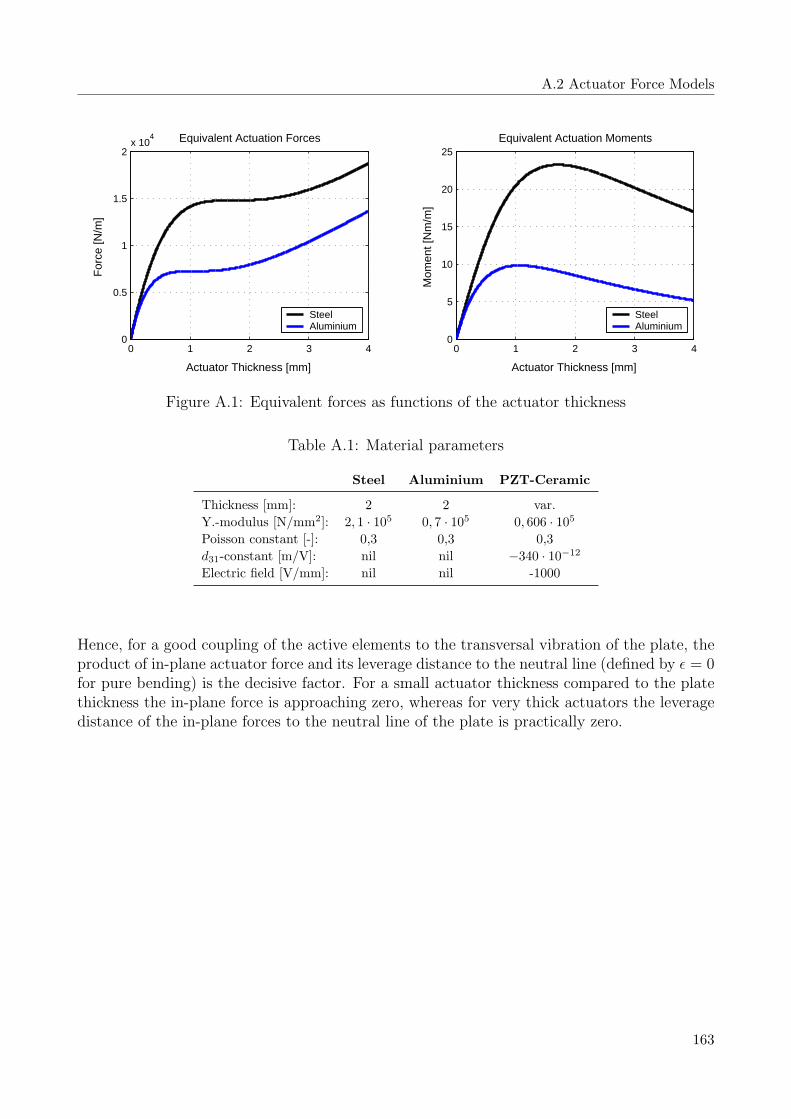
A.2 Actuator Force Models
0 1 2 3 40
0.5
1
1.5
2x 10
4 Equivalent Actuation Forces
Actuator Thickness [mm]
For
ce [N
/m]
SteelAluminium
0 1 2 3 40
5
10
15
20
25Equivalent Actuation Moments
Actuator Thickness [mm]
Mom
ent [
Nm
/m]
SteelAluminium
Figure A.1: Equivalent forces as functions of the actuator thickness
Table A.1: Material parameters
Steel Aluminium PZT-Ceramic
Thickness [mm]: 2 2 var.
Y.-modulus [N/mm2]: 2, 1 · 105 0, 7 · 105 0, 606 · 105
Poisson constant [-]: 0,3 0,3 0,3
d31-constant [m/V]: nil nil −340 · 10−12
Electric field [V/mm]: nil nil -1000
Hence, for a good coupling of the active elements to the transversal vibration of the plate, theproduct of in-plane actuator force and its leverage distance to the neutral line (defined by ǫ = 0for pure bending) is the decisive factor. For a small actuator thickness compared to the platethickness the in-plane force is approaching zero, whereas for very thick actuators the leveragedistance of the in-plane forces to the neutral line of the plate is practically zero.
163

Appendix B
Technical Drawings
10,6
423
18 5
M2.5
32
34
3
8,35,9
19
0,2
Clamshell Actuator Unit
Figure B.1: Clamshell actuator unit

62
3
16,6
22,610,6
M4
Active Attachment Element
R26,5
R21,5
Figure B.2: Active attachment element
165

Appendix C
Experimental Investigation
C.1 Test Structure
C.1.1 Material Parameters Fuselage Panel
The CFRP skin panel is stiffened by five CFRP-stringers (structurally integrated into theskin, spacing 175 mm) and two perpendicular CFRP-frames (riveted to the skin and stringersrespectively, spacing 533 mm). Materials and stacking sequence for the skin panel are listedin Table C.1.
Table C.1: Material parameters fuselage skin
Layer Material∗ and Orientation∗∗
1 Cytec Adhesive Film BMS5-154 TY2CL1GR5 Melt Bond 1515
2 Expanded foil
3 Fiberite Dry fabric 3k70-T400H-PW, 0, 90
4 Saertex Multiaxial fabric IM7-12K, 0, +45, -45
5 Saertex Multiaxial fabric IM7-12K, -45, +45, 0
6 Saertex Multiaxial fabric IM7-12K, 0, +45, -45
7 Saertex Multiaxial fabric IM7-12K, +45, -45, 0
8 Fiberite Dry fabric 3k70-T400H-PW, 0, 90
9 Saertex Multiaxial fabric IM7-12K, 0, +45, 0, -45
10 Saertex Multiaxial fabric IM7-12K, 0, 90, 0
∗ manufactured in resin infusion technique, epoxy resin type 977-2-1000gsm(Cytec); ∗∗ 0 direction is defined along the stringer direction
The stringers are made from a braided tube reinforced with a prepreg bulb:
• Foot and web: braided triaxial sleeving in carbon fibre HTA-6K ID 58 mm - FAW 917gmq, Wth 0,86 mm, 167 g/m - 58% 0, 42% ±57
• Bulb: carbon fibre prepreg Tape HYE 977-2/ HTA-12K / 35 268/ 300, TH. 0.25, DAN432 REV. 2, (Cytec/Fiberite)
The frames are built in a C-sectioned design and have a total thickness of 3,75 mm. The frameheight is 90 mm, while the length of the flange is 35 mm:

C.1 Test Structure
• Material: carbon fibre HTS/977-2, thickness 0,25 mm for one single ply
• Stacking sequence: -45, 0, 0, 90, 0, 0, 45, 0, 45, 0, 0, 90, 0, 0, -45 (60% 0,27% ±45, 13% 90)
C.1.2 Material Parameters Trim Panel
Table C.2: Material parameters trim panel 1
Layer Material∗
1 Hexcel V260/38/7781 fibreglass fabric
2 Nomex HRH 10 3/16.2, thickness 8 mm
3 Hexcel V260/38/7781 fibreglass fabric
4 Hexcel V260/60/1080 fibreglass fabric
5 PVF film (cabin side)
∗ honeycomb core trim panel, phenolique resin system
Table C.3: Material parameters trim panel 2
Layer Material∗
1 PN 900-C08-45 carbon fibre fabric, thickness 0,18 mm
2 LN 29964-A2 Nomex honeycomb core, thickness 4 mm
3 PN 900-C08-45 carbon fibre fabric, thickness 0,18 mm
4 PN 900-44-43 fibreglass fabric, thickness 0,09 mm
∗ honeycomb core trim panel, cyanate-ester resin system
167
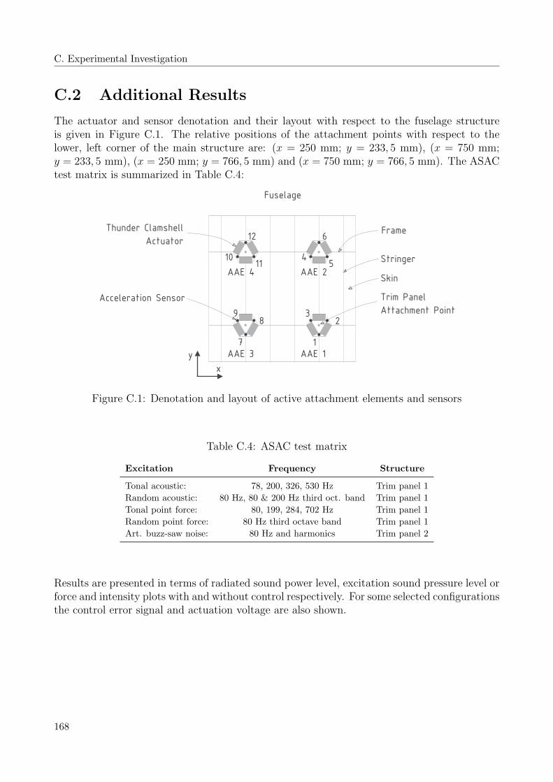
C. Experimental Investigation
C.2 Additional Results
The actuator and sensor denotation and their layout with respect to the fuselage structureis given in Figure C.1. The relative positions of the attachment points with respect to thelower, left corner of the main structure are: (x = 250 mm; y = 233, 5 mm), (x = 750 mm;y = 233, 5 mm), (x = 250 mm; y = 766, 5 mm) and (x = 750 mm; y = 766, 5 mm). The ASACtest matrix is summarized in Table C.4:
Thunder Clamshell
Actuator
Stringer
Frame
Skin
Fuselage
Trim Panel
Attachment Point
y
x
AAE 1AAE 3
AAE 2AAE 4
7
6
29 3
41011 5
8
1
12
Acceleration Sensor
Figure C.1: Denotation and layout of active attachment elements and sensors
Table C.4: ASAC test matrix
Excitation Frequency Structure
Tonal acoustic: 78, 200, 326, 530 Hz Trim panel 1
Random acoustic: 80 Hz, 80 & 200 Hz third oct. band Trim panel 1
Tonal point force: 80, 199, 284, 702 Hz Trim panel 1
Random point force: 80 Hz third octave band Trim panel 1
Art. buzz-saw noise: 80 Hz and harmonics Trim panel 2
Results are presented in terms of radiated sound power level, excitation sound pressure level orforce and intensity plots with and without control respectively. For some selected configurationsthe control error signal and actuation voltage are also shown.
168
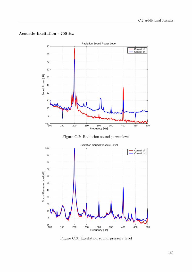
C.2 Additional Results
Acoustic Excitation - 200 Hz
100 150 200 250 300 350 400 450 500−10
0
10
20
30
40
50
60
70
80
90Radiation Sound Power Level
Frequency [Hz]
Sou
nd P
ower
[dB
]
Control offControl on
Figure C.2: Radiation sound power level
100 150 200 250 300 350 400 450 500−10
0
10
20
30
40
50
60
70
80
90
100Excitation Sound Pressure Level
Frequency [Hz]
Sou
nd P
ress
ure
Leve
l [dB
]
Control offControl on
Figure C.3: Excitation sound pressure level
169
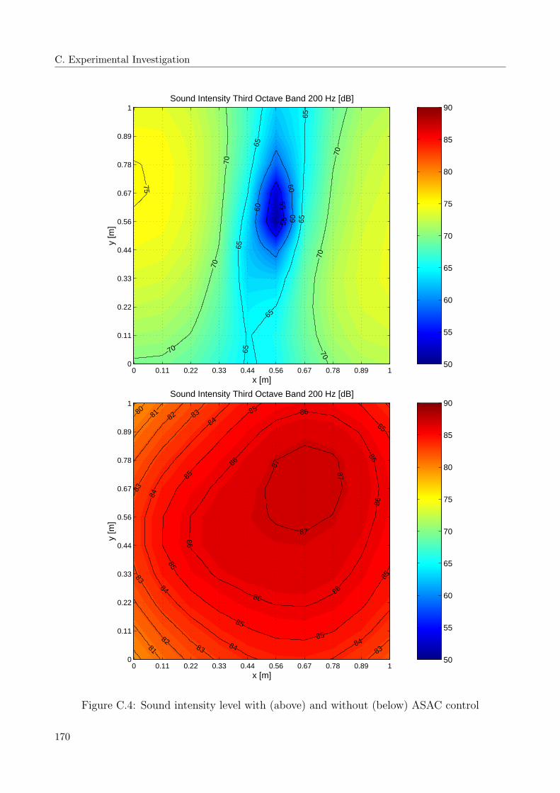
C. Experimental Investigation
50
55
60
65
70
75
80
85
90
x [m]
y [m
]Sound Intensity Third Octave Band 200 Hz [dB]
5555
60
60
60
6565
65
65
6565
70
70
70 70
70
70
75
0 0.11 0.22 0.33 0.44 0.56 0.67 0.78 0.89 10
0.11
0.22
0.33
0.44
0.56
0.67
0.78
0.89
1
50
55
60
65
70
75
80
85
90
x [m]
y [m
]
Sound Intensity Third Octave Band 200 Hz [dB]
8081
81 82
82
83
83
83
83
83
84
84
84
84 84
85
85
85
85
85
85
85
86
8686
86
86
86
86
87
87
87
0 0.11 0.22 0.33 0.44 0.56 0.67 0.78 0.89 10
0.11
0.22
0.33
0.44
0.56
0.67
0.78
0.89
1
Figure C.4: Sound intensity level with (above) and without (below) ASAC control
170

C.2 Additional Results
Acoustic Excitation - 326 Hz
200 250 300 350 400 450 5000
10
20
30
40
50
60
70
80Radiation Sound Power Level
Frequency [Hz]
Sou
nd P
ower
[dB
]
Control offControl on
Figure C.5: Radiation sound power level
200 250 300 350 400 450 500−10
0
10
20
30
40
50
60
70
80
90
100Excitation Sound Pressure Level
Frequency [Hz]
Sou
nd P
ress
ure
Leve
l [dB
]
Control offControl on
Figure C.6: Excitation sound pressure level
171

C. Experimental Investigation
40
45
50
55
60
65
70
75
x [m]
y [m
]Sound Intensity Third Octave Band 315 Hz [dB]
30
40
40
40
40
50
50
50
50
60
60
60
60
60 6060
60
0 0.11 0.22 0.33 0.44 0.56 0.67 0.78 0.89 10
0.11
0.22
0.33
0.44
0.56
0.67
0.78
0.89
1
40
45
50
55
60
65
70
75
x [m]
y [m
]
Sound Intensity Third Octave Band 315 Hz [dB]
55
55
60
60
60
65
65
65
65
65
65
65
70
70
70
70
70
70
70
75
75
75
0 0.11 0.22 0.33 0.44 0.56 0.67 0.78 0.89 10
0.11
0.22
0.33
0.44
0.56
0.67
0.78
0.89
1
Figure C.7: Sound intensity level with (above) and without (below) ASAC control
172
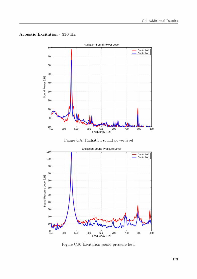
C.2 Additional Results
Acoustic Excitation - 530 Hz
450 500 550 600 650 700 750 800 850−10
0
10
20
30
40
50
60
70
80Radiation Sound Power Level
Frequency [Hz]
Sou
nd P
ower
[dB
]
Control offControl on
Figure C.8: Radiation sound power level
450 500 550 600 650 700 750 800 8500
10
20
30
40
50
60
70
80
90
100
110Excitation Sound Pressure Level
Frequency [Hz]
Sou
nd P
ress
ure
Leve
l [dB
]
Control offControl on
Figure C.9: Excitation sound pressure level
173

C. Experimental Investigation
40
45
50
55
60
65
70
75
80
x [m]
y [m
]Sound Intensity Third Octave Band 500 Hz [dB]
45
5050
55
55
55
55
55
60
60
60
60
60
60
60
60
60
60
60
60
65
65
65
65
65
65
65
65
65
65
0 0.11 0.22 0.33 0.44 0.56 0.67 0.78 0.89 10
0.11
0.22
0.33
0.44
0.56
0.67
0.78
0.89
1
40
45
50
55
60
65
70
75
80
x [m]
y [m
]
Sound Intensity Third Octave Band 500 Hz [dB]
20
20
30
30
30
30
40
40
40
40
50
50
50
50
50
50
60
60
60
60
60
60 60
60
70
70
70 70
70
70
70
70
80
80
0 0.11 0.22 0.33 0.44 0.56 0.67 0.78 0.89 10
0.11
0.22
0.33
0.44
0.56
0.67
0.78
0.89
1
Figure C.10: Sound intensity level with (above) and without (below) ASAC control
174
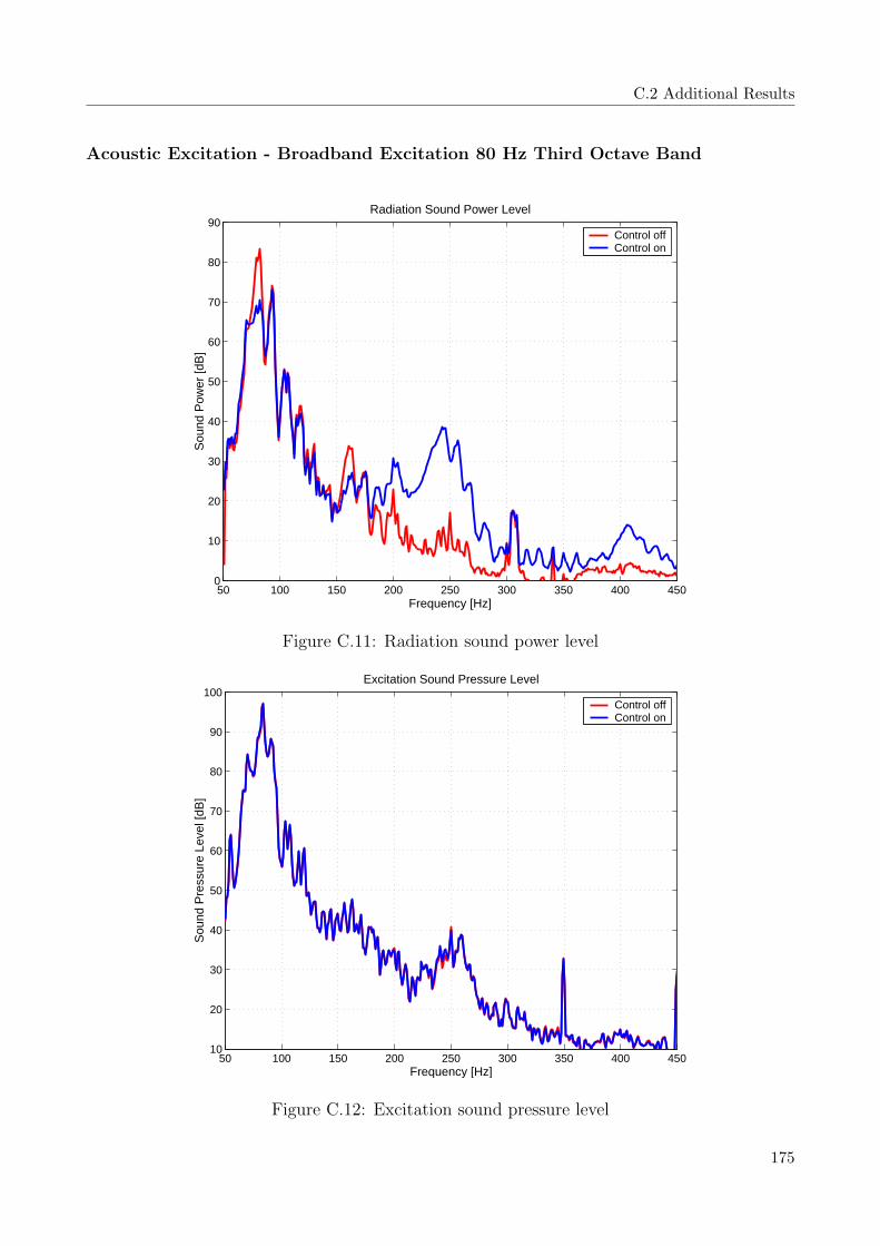
C.2 Additional Results
Acoustic Excitation - Broadband Excitation 80 Hz Third Octave Band
50 100 150 200 250 300 350 400 4500
10
20
30
40
50
60
70
80
90Radiation Sound Power Level
Frequency [Hz]
Sou
nd P
ower
[dB
]
Control offControl on
Figure C.11: Radiation sound power level
50 100 150 200 250 300 350 400 45010
20
30
40
50
60
70
80
90
100Excitation Sound Pressure Level
Frequency [Hz]
Sou
nd P
ress
ure
Leve
l [dB
]
Control offControl on
Figure C.12: Excitation sound pressure level
175

C. Experimental Investigation
72
74
76
78
80
82
84
86
88
x [m]
y [m
]Sound Intensity Third Octave Band 80 Hz [dB]
73
74
74
74
74
74
74
7474
75
75
7575
7575
75
75
76
76
76
76
76
7677
77
7777
77
77
0 0.11 0.22 0.33 0.44 0.56 0.67 0.78 0.89 10
0.11
0.22
0.33
0.44
0.56
0.67
0.78
0.89
1
72
74
76
78
80
82
84
86
88
x [m]
y [m
]
Sound Intensity Third Octave Band 80 Hz [dB]
83
84
84
84
84
84
84
84
84
85
85
85
85
85
85
85
85
85
85
85
8686
86
86
86
86
86
8687
87
87
87
87
0 0.11 0.22 0.33 0.44 0.56 0.67 0.78 0.89 10
0.11
0.22
0.33
0.44
0.56
0.67
0.78
0.89
1
Figure C.13: Sound intensity level with (above) and without (below) ASAC control
176

C.2 Additional Results
Acoustic Excitation - Broadband Excitation 80 and 200 Hz Third Octave Band
50 100 150 200 250 300 350 400 450 500 5500
10
20
30
40
50
60
70
80
90Radiation Sound Power Level
Frequency [Hz]
Sou
nd P
ower
[dB
]
Control offControl on
Figure C.14: Radiation sound power level
50 100 150 200 250 300 350 400 450 500 55020
30
40
50
60
70
80
90
100Excitation Sound Pressure Level
Frequency [Hz]
Sou
nd P
ress
ure
Leve
l [dB
]
Control offControl on
Figure C.15: Excitation sound pressure level
177

C. Experimental Investigation
77
78
79
80
81
82
83
84
85
86
87
88
x [m]
y [m
]Sound Intensity Third Octave Band 80 Hz [dB]
78
79
79
79
79
79
79
79
80
80
80
80
80
80
80
80
80
80
81
81
81
81
81
81
82
82
82
82
0 0.11 0.22 0.33 0.44 0.56 0.67 0.78 0.89 10
0.11
0.22
0.33
0.44
0.56
0.67
0.78
0.89
1
77
78
79
80
81
82
83
84
85
86
87
88
x [m]
y [m
]
Sound Intensity Third Octave Band 80 Hz [dB]
83
83
83
83
84
84
84
84
84
84
84
85
8585
85
85
85
8585
85
85
85
86
86
86
86
86
86
86
86
86
8787
87
87
0 0.11 0.22 0.33 0.44 0.56 0.67 0.78 0.89 10
0.11
0.22
0.33
0.44
0.56
0.67
0.78
0.89
1
Figure C.16: Sound intensity level with (above) and without (below) ASAC control
178

C.2 Additional Results
74
76
78
80
82
84
86
x [m]
y [m
]Sound Intensity Third Octave Band 200 Hz [dB]
78
79
79
79
79
79
79
7980
80
80
80
80
80
80
80
8080
81
8181
81
81
81
82
82
82
82
74
74
75
75
75
75
76
76
76
76
76
76
76
76
77
77
77
77
77
77
77
7778
78
78
78
79
79
80
0 0.11 0.22 0.33 0.44 0.56 0.67 0.78 0.89 10
0.11
0.22
0.33
0.44
0.56
0.67
0.78
0.89
1
74
76
78
80
82
84
86
x [m]
y [m
]
Sound Intensity Third Octave Band 200 Hz [dB]
83
83
83
83
83
84
84
84
84
84
84
84
85
8585
85
85
85
85
85
85
85
85
86
86
86
86
86
86
86
86
86
8787
87
87
81
82
82
83
83
8383
83
84 84
84
8484
84
84
85
85
85
85
85
85
0 0.11 0.22 0.33 0.44 0.56 0.67 0.78 0.89 10
0.11
0.22
0.33
0.44
0.56
0.67
0.78
0.89
1
Figure C.17: Sound intensity level with (above) and without (below) ASAC control
179

C. Experimental Investigation
0 2 4 6 8 10−0.02
−0.015
−0.01
−0.005
0
0.005
0.01
0.015
0.02Sensor 6 − Attachment Element 2
Time [s]
Vel
ocity
[m/s
]
Control offControl on
0 2 4 6 8 10−0.02
−0.015
−0.01
−0.005
0
0.005
0.01
0.015
0.02Sensor 21 − Trim Panel
Time [s]
Vel
ocity
[m/s
]
Control offControl on
0 0.02 0.04 0.06 0.08 0.1−0.02
−0.015
−0.01
−0.005
0
0.005
0.01
0.015
0.02Sensor 6 − Attachment Element 2
Time [s]
Vel
ocity
[m/s
]
Control offControl on
0 0.02 0.04 0.06 0.08 0.1−0.02
−0.015
−0.01
−0.005
0
0.005
0.01
0.015
0.02Sensor 21 − Trim Panel
Time [s]
Vel
ocity
[m/s
]
Control offControl on
Figure C.18: Velocity measured by error sensor 6 and 21, with and without control
100 200 300 400 500−100
−90
−80
−70
−60
−50
−40
Frequency [Hz]
Err
or S
igna
l [dB
(1m
/s)]
Velocity Error Signal − Trim Panel
Control offControl on
100 200 300 400 500−100
−90
−80
−70
−60
−50
−40
Frequency [Hz]
Err
or S
igna
l [dB
(1m
/s)]
Velocity Error Signal − AAE
Control offControl on
Figure C.19: Squared sum of error signals on trim panel and attachment elements
180

C.2 Additional Results
0 0.02 0.04 0.06 0.08 0.1−50
−40
−30
−20
−10
0
10
20
30
40
50Attachment Element 1
Time [s]
Vol
tage
[V]
Actuator 1Actuator 2Actuator 3
0 0.02 0.04 0.06 0.08 0.1−50
−40
−30
−20
−10
0
10
20
30
40
50Attachment Element 2
Time [s]
Vol
tage
[V]
Actuator 4Actuator 5Actuator 6
0 0.02 0.04 0.06 0.08 0.1−50
−40
−30
−20
−10
0
10
20
30
40
50Attachment Element 3
Time [s]
Vol
tage
[V]
Actuator 7Actuator 8Actuator 9
0 0.02 0.04 0.06 0.08 0.1−50
−40
−30
−20
−10
0
10
20
30
40
50Attachment Element 4
Time [s]
Vol
tage
[V]
Actuator 10Actuator 11Actuator 12
Figure C.20: Actuator voltage
181

C. Experimental Investigation
Point Force Excitation - 80 and 199 Hz
50 100 150 200 250 300 350 400 4500
10
20
30
40
50
60
70
80
90
100Radiation Sound Power Level
Frequency [Hz]
Sou
nd P
ower
[dB
]
Control offControl on
Figure C.21: Radiation sound power level
50 100 150 200 250 300 350 400 45010
−5
10−4
10−3
10−2
10−1
100
101
Excitation Force
Frequency [Hz]
For
ce [N
]
Control offControl on
Figure C.22: Excitation force
182

C.2 Additional Results
70
75
80
85
90
95
x [m]
y [m
]Sound Intensity Third Octave Band 80 Hz [dB]
69
70
70
70
70
71
71
71
71
71
71
71
71
72
72
72
72
7272
72
73
73
73
73
73
74
74
74
0 0.11 0.22 0.33 0.44 0.56 0.67 0.78 0.89 10
0.11
0.22
0.33
0.44
0.56
0.67
0.78
0.89
1
70
75
80
85
90
95
x [m]
y [m
]
Sound Intensity Third Octave Band 80 Hz [dB]
93
94
94
94
9495
95
95
95 95
95
95
95
96
96
96
96
96
96
97
97
97
97
0 0.11 0.22 0.33 0.44 0.56 0.67 0.78 0.89 10
0.11
0.22
0.33
0.44
0.56
0.67
0.78
0.89
1
Figure C.23: Sound intensity level with (above) and without (below) ASAC control
183

C. Experimental Investigation
50
55
60
65
70
75
80
85
90
x [m]
y [m
]Sound Intensity Third Octave Band 200 Hz [dB]
45
5050
55
55
60
60
65
65
70
70
70
75
75 75
75
80
80
80
8080
80
0 0.11 0.22 0.33 0.44 0.56 0.67 0.78 0.89 10
0.11
0.22
0.33
0.44
0.56
0.67
0.78
0.89
1
50
55
60
65
70
75
80
85
90
x [m]
y [m
]
Sound Intensity Third Octave Band 200 Hz [dB]
7880
82
84
84
84
86
86
86
88
88
88
90
90
90
90
92
92
92
92
92
0 0.11 0.22 0.33 0.44 0.56 0.67 0.78 0.89 10
0.11
0.22
0.33
0.44
0.56
0.67
0.78
0.89
1
Figure C.24: Sound intensity level with (above) and without (below) ASAC control
184
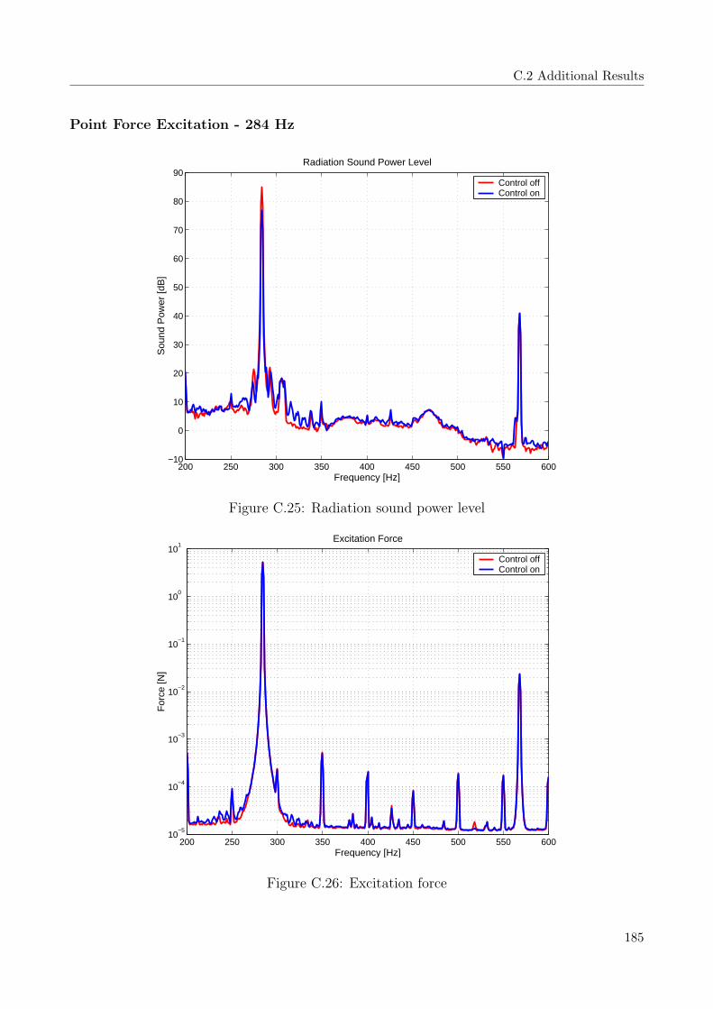
C.2 Additional Results
Point Force Excitation - 284 Hz
200 250 300 350 400 450 500 550 600−10
0
10
20
30
40
50
60
70
80
90Radiation Sound Power Level
Frequency [Hz]
Sou
nd P
ower
[dB
]
Control offControl on
Figure C.25: Radiation sound power level
200 250 300 350 400 450 500 550 60010
−5
10−4
10−3
10−2
10−1
100
101
Excitation Force
Frequency [Hz]
For
ce [N
]
Control offControl on
Figure C.26: Excitation force
185

C. Experimental Investigation
60
65
70
75
80
85
x [m]
y [m
]Sound Intensity Third Octave Band 315 Hz [dB]
60
60 6565
65 65
70
70
70
70
70
75
75
75
75
80
80
0 0.11 0.22 0.33 0.44 0.56 0.67 0.78 0.89 10
0.11
0.22
0.33
0.44
0.56
0.67
0.78
0.89
1
60
65
70
75
80
85
x [m]
y [m
]
Sound Intensity Third Octave Band 315 Hz [dB]
65
70
70
75
75
75
75
80
80
80
80
80
80
80
85
85
85
85
0 0.11 0.22 0.33 0.44 0.56 0.67 0.78 0.89 10
0.11
0.22
0.33
0.44
0.56
0.67
0.78
0.89
1
Figure C.27: Sound intensity level with (above) and without (below) ASAC control
186

C.2 Additional Results
Point Force Excitation - 702 Hz
600 650 700 750 800 850 900 950 1000−20
−10
0
10
20
30
40
50
60
70
80Radiation Sound Power Level
Frequency [Hz]
Sou
nd P
ower
[dB
]
Control offControl on
Figure C.28: Radiation sound power level
600 650 700 750 800 850 900 950 100010
−5
10−4
10−3
10−2
10−1
100
101
Excitation Force
Frequency [Hz]
For
ce [N
]
Control offControl on
Figure C.29: Excitation force
187

C. Experimental Investigation
40
45
50
55
60
65
70
75
80
x [m]
y [m
]Sound Intensity Third Octave Band 630 Hz [dB]
40
50
50
60 60
60
60
60
60
60
60 60
60
60
60
60
606060
70
0 0.11 0.22 0.33 0.44 0.56 0.67 0.78 0.89 10
0.11
0.22
0.33
0.44
0.56
0.67
0.78
0.89
1
40
45
50
55
60
65
70
75
80
x [m]
y [m
]
Sound Intensity Third Octave Band 630 Hz [dB]
40
40
40
40
40
50
50
50
50
50
50
50
6060
60
60
60
60
60
60
60
60
60
70
70
70
7070
70
70
70
70
70
70
70
0 0.11 0.22 0.33 0.44 0.56 0.67 0.78 0.89 10
0.11
0.22
0.33
0.44
0.56
0.67
0.78
0.89
1
Figure C.30: Sound intensity level with (above) and without (below) ASAC control
188

C.2 Additional Results
Point Force Excitation - Broadband Excitation 80 Hz Third Octave Band
0 50 100 150 200 250 300 350 4000
10
20
30
40
50
60
70
80Radiation Sound Power Level
Frequency [Hz]
Sou
nd P
ower
[dB
]
Control offControl on
Figure C.31: Radiation sound power level
0 50 100 150 200 250 300 350 40010
−5
10−4
10−3
10−2
10−1
100
Excitation Force
Frequency [Hz]
For
ce [N
]
Control offControl on
Figure C.32: Excitation force
189

C. Experimental Investigation
74
76
78
80
82
84
86
x [m]
y [m
]Sound Intensity Third Octave Band 80 Hz [dB]
73
74
74
74
74
74
74
74
7474
75
7575
75
75
75
75
75
76
76
76
76
76
76
77
77
0 0.11 0.22 0.33 0.44 0.56 0.67 0.78 0.89 10
0.11
0.22
0.33
0.44
0.56
0.67
0.78
0.89
1
74
76
78
80
82
84
86
x [m]
y [m
]
Sound Intensity Third Octave Band 80 Hz [dB]
81
82
82
8282
82
83
8383
83
83
83
83
83
83
83
84
84
84
84
84
84
84
85
85
85
85
85
86
86
0 0.11 0.22 0.33 0.44 0.56 0.67 0.78 0.89 10
0.11
0.22
0.33
0.44
0.56
0.67
0.78
0.89
1
Figure C.33: Sound intensity level with (above) and without (below) ASAC control
190
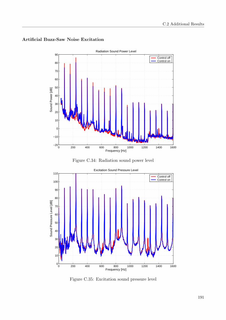
C.2 Additional Results
Artificial Buzz-Saw Noise Excitation
0 200 400 600 800 1000 1200 1400 1600−20
−10
0
10
20
30
40
50
60
70
80
90Radiation Sound Power Level
Frequency [Hz]
Sou
nd P
ower
[dB
]
Control offControl on
Figure C.34: Radiation sound power level
0 200 400 600 800 1000 1200 1400 16000
10
20
30
40
50
60
70
80
90
100
110Excitation Sound Pressure Level
Frequency [Hz]
Sou
nd P
ress
ure
Leve
l [dB
]
Control offControl on
Figure C.35: Excitation sound pressure level
191

C. Experimental Investigation
0 2 4 6 8 10−2.5
−2
−1.5
−1
−0.5
0
0.5
1
1.5
2
2.5Sensor 6 − Attachment Element 2
Time [s]
Acc
eler
atio
n [g
]
Control offControl on
0 2 4 6 8 10−2.5
−2
−1.5
−1
−0.5
0
0.5
1
1.5
2
2.5Sensor 21 − Trim Panel
Time [s]
Acc
eler
atio
n [g
]
Control offControl on
0 0.01 0.02 0.03 0.04 0.05−2.5
−2
−1.5
−1
−0.5
0
0.5
1
1.5
2
2.5Sensor 6 − Attachment Element 2
Time [s]
Acc
eler
atio
n [g
]
Control offControl on
0 0.01 0.02 0.03 0.04 0.05−2.5
−2
−1.5
−1
−0.5
0
0.5
1
1.5
2
2.5Sensor 21 − Trim Panel
Time [s]
Acc
eler
atio
n [g
]
Control offControl on
Figure C.36: Acceleration measured by error sensor 6 and 21, with and without control
0 500 1000 1500−80
−70
−60
−50
−40
−30
−20
−10
0
10
Frequency [Hz]
Err
or S
igna
l [dB
(1g)
]
Acceleration Error Signal − Trim Panel
Control offControl on
0 500 1000 1500−80
−70
−60
−50
−40
−30
−20
−10
0
10
Frequency [Hz]
Err
or S
igna
l [dB
(1g)
]
Acceleration Error Signal − AAE
Control offControl on
Figure C.37: Squared sum of error signals on trim panel and attachment elements
192

C.2 Additional Results
0 0.01 0.02 0.03 0.04 0.05−100
−50
0
50
100Attachment Element 1
Time [s]
Vol
tage
[V]
Actuator 1Actuator 2Actuator 3
0 0.01 0.02 0.03 0.04 0.05−100
−50
0
50
100Attachment Element 2
Time [s]
Vol
tage
[V]
Actuator 4Actuator 5Actuator 6
0 0.01 0.02 0.03 0.04 0.05−100
−50
0
50
100Attachment Element 3
Time [s]
Vol
tage
[V]
Actuator 7Actuator 8Actuator 9
0 0.01 0.02 0.03 0.04 0.05−100
−50
0
50
100Attachment Element 4
Time [s]
Vol
tage
[V]
Actuator 10Actuator 11Actuator 12
Figure C.38: Actuator voltage
193