
Diploma Thesis - Pàgina inicial de UPCommons€¦ · · 2017-02-09of high and low temperature...
131
Transcript of Diploma Thesis - Pàgina inicial de UPCommons€¦ · · 2017-02-09of high and low temperature...
Diploma Thesis
von cand. Ing. Elisa Jubany Arribas
Thermodynamic Model of a
Cascaded Organic Rankine
Cycle Power Plant
Supervisor: Dipl.-Ing.Gabor Ast (external)
Dipl.-Ing.Richard Aumann (internal)
Prof. Dr.-Ing. Hartmut Splietho� (internal)
Issued: 15.06.2010
Submitted: 15.12.2010


Declaration of Authorship
Hiermit versichere ich, die vorliegende Arbeit selbständig und ohne Hilfe Drit-
ter angefertigt zu haben. Gedanken und Zitate, die ich aus fremden Quellen
direkt oder indirekt übernommen habe, sind als solche kenntlich gemacht.
Diese Arbeit hat in gleicher oder ähnlicher Form noch keiner Prüfungsbe-
hörde vorgelegen und wurde bisher nicht verö�entlicht.
Ich erkläre mich damit einverstanden, dass die Arbeit durch den Lehrstuhl
für Energiesysteme der Ö�entlichkeit zugänglich gemacht werden kann.
,

Acknowledgements
This diploma thesis was conducted at the Alternative Energy Lab at GE
Global Research Europe (GEGR) in cooperation with the Institute of En-
ergy Systems (ES) at Technische Universität München.
First and foremost, I would like to sincerely thank my GE supervisors Gabor
Ast and Monika Muehlbauer for leading, helping and supporting me in the
course of this work. I want to express them my deep gratitude for the trust
they put in me. They helped me to develop an understanding of the subject
and their advice and knowledge were very precious to me. I cannot forget
about my tutor Richard Aumann from Technische Universität München for
o�ering me the opportunity to participate in this project in GEGR and for
following and supporting my progress.
I would also like to show my gratitude to the other members of the AEL/ATL
laboratories who did not doubt in helping me whenever I needed them, spe-
cially my colleges from the waste heat recovery team Sebastian, Pierre and
Matt. I always found an open door for discussion and questions. Thanks
as well to to my o�ce mates, especially to Andreas, Hannes, Lucas, Nick,
Yannick, and Antonius for their help and encouragement, and for the great
time we spent together.
Of course, I would have never been able to accomplish my goals without the
support of my family and friends, with special mention for my parents.
And �nally, I would like to express all my gratitude to Sara and Guim for
their support and patience and for encouraging me in many ways.


Abstract
The Alternative Energy Lab at GE Global Research has fully developed a
functional power plant to recover waste heat from a Jenbacher engine using
a Cascaded Organic Rankine Cycle. This solution is required to produce ad-
ditional electricity, by using the heat rejected by an engine without changing
or disturbing its way of functioning. Therefore, it is particularly important
that such systems can adapt to changes in the gas engine operating point and
hence changes in the amount of waste heat given to the system. Moreover
the system has to conserve a good e�ciency when ambient conditions are
changing.
This novel cycle concept reaches a high e�ciency by separating the recovery
of high and low temperature sources of the J420 GS Jenbacher engine. In-
deed the J420 GS is a 1451 kW gas engine working with biogas and rejecting
heat to the ambient atmosphere through two temperature sources, which are
potential sources for the CORE cycle: a low temperature source, constituted
by the engine cooling water system and a high temperature source consti-
tuted by the exhaust gas stream going out of the engine.
Scope of this thesis is the establishment of a thermodynamic model of the
CO.Ra product. EBSILON will be the platform for the development of the
model. This thesis is the �rst work at GE Global Research Munich using
this simulation software. Therefore, the main scope of this work is to �nd
out whether EBSILON is suitable or not to run ORC simulations both under

design and o�-design conditions. For this purpose, the current EBSILON
component capabilities will be studied. To match the simulation require-
ments the standard components will be extended.
Once the model is assembled in design and o�-design mode, o�-design simula-
tions will be performed. The focus of the steady-state o�-design simulations
carried out in this study is on the one hand, the sensitivity analysis of the
model and on the other hand the calculation of the rotary speed of pumps
in order to operate the plant close to the design point.
vi
Contents
Declaration of Authorship i
Acknowledgements iii
Abstract v
Table of Contents ix
List of Figures xii
List of Tables xiii
Nomenclature xv
1 Introduction 1
1.1 World Energy Tendencies . . . . . . . . . . . . . . . . . . . . 1
1.2 Waste Heat Recovery . . . . . . . . . . . . . . . . . . . . . . . 3
1.3 De�nition of Goals . . . . . . . . . . . . . . . . . . . . . . . . 6
2 Technical Overview 9
2.1 Thermodynamic Cycles . . . . . . . . . . . . . . . . . . . . . . 9
2.1.1 Rankine Cycle . . . . . . . . . . . . . . . . . . . . . . . 9
2.1.2 Organic Rankine Cycle . . . . . . . . . . . . . . . . . . 11
2.1.3 Cascaded Organic Rankine Cycle . . . . . . . . . . . . 13
2.2 O�-Design Background . . . . . . . . . . . . . . . . . . . . . . 15

3 Used Software:EBSILON 17
3.1 Main Features . . . . . . . . . . . . . . . . . . . . . . . . . . . 17
3.2 Comparison of EBSILON and HYSYS . . . . . . . . . . . . . 20
4 Plant Design 23
4.1 Heat Source . . . . . . . . . . . . . . . . . . . . . . . . . . . . 25
4.2 Working Fluid Properties . . . . . . . . . . . . . . . . . . . . . 27
4.3 Plant Description . . . . . . . . . . . . . . . . . . . . . . . . . 30
4.3.1 Thermal Oil Loop . . . . . . . . . . . . . . . . . . . . . 30
4.3.2 High Temperature Loop . . . . . . . . . . . . . . . . . 32
4.3.3 Low Temperature Loop . . . . . . . . . . . . . . . . . . 34
4.4 Design Point . . . . . . . . . . . . . . . . . . . . . . . . . . . . 36
5 Extended Component Models 41
5.1 Heat Exchanger Model . . . . . . . . . . . . . . . . . . . . . . 41
5.1.1 Technical Background . . . . . . . . . . . . . . . . . . 41
5.1.2 Design Calculation . . . . . . . . . . . . . . . . . . . . 42
5.1.3 O�-design Calculation . . . . . . . . . . . . . . . . . . 45
5.1.4 Issues in modelling . . . . . . . . . . . . . . . . . . . . 47
5.2 Pump Model . . . . . . . . . . . . . . . . . . . . . . . . . . . 51
5.2.1 Technical Background . . . . . . . . . . . . . . . . . . 51
5.2.2 Design Calculation . . . . . . . . . . . . . . . . . . . . 54
5.2.3 O�-design Calculation . . . . . . . . . . . . . . . . . . 54
5.2.4 Issues in modelling . . . . . . . . . . . . . . . . . . . . 58
5.3 Expander Model . . . . . . . . . . . . . . . . . . . . . . . . . 60
5.3.1 Technical Background . . . . . . . . . . . . . . . . . . 60
5.3.2 Design Calculation . . . . . . . . . . . . . . . . . . . . 61
5.3.3 O�-design Calculation . . . . . . . . . . . . . . . . . . 61
5.3.4 Issues in modelling . . . . . . . . . . . . . . . . . . . . 64
6 Switch from Design to O�-Design 67
6.1 Component Adjustments . . . . . . . . . . . . . . . . . . . . . 68
viii
CONTENTS
6.2 Cycle Adjustments . . . . . . . . . . . . . . . . . . . . . . . . 70
7 O�-design Simulations 75
7.1 O�-design model . . . . . . . . . . . . . . . . . . . . . . . . . 75
7.2 Sensitivity Analysis . . . . . . . . . . . . . . . . . . . . . . . . 78
8 Outlook and Conclusion 87
Bibliography 93
Appendix 95
A.1 Ebsilon Legend . . . . . . . . . . . . . . . . . . . . . . . . . . 95
A.2 Thermal Oil Data . . . . . . . . . . . . . . . . . . . . . . . . . 96
A.3 Plant Components . . . . . . . . . . . . . . . . . . . . . . . . 97
ix

List of Figures
1.1 World Energy Consumption and Production . . . . . . . . . . 2
1.2 Carbon Dioxide Emissions by Sector and Fuel . . . . . . . . . 3
1.3 Energy Content of U.S. Industry Thermal Emissions . . . . . 4
1.4 Heat Sources for Waste Heat Recovery . . . . . . . . . . . . . 5
2.1 Rankine Cycle . . . . . . . . . . . . . . . . . . . . . . . . . . . 10
2.2 Main Components of the ORC . . . . . . . . . . . . . . . . . . 12
2.3 E�ect of molecule size on the slope . . . . . . . . . . . . . . . 12
2.4 Cascaded Organic Rankine Cycle . . . . . . . . . . . . . . . . 14
3.1 Hierarchy Tree . . . . . . . . . . . . . . . . . . . . . . . . . . 18
3.2 KernelScripting:Pump Model . . . . . . . . . . . . . . . . . . 19
4.1 Schematic representation of CO.Ra . . . . . . . . . . . . . . . 24
4.2 Sankey diagram of the J 420 GS . . . . . . . . . . . . . . . . . 26
4.3 T-s-diagramm of water-steam,R245fa and cyclohexane . . . . . 29
4.4 Design Speci�cations in the Thermal Oil Loop . . . . . . . . . 30
4.5 Design Speci�cations in the High Temperature Loop . . . . . . 33
4.6 Design Speci�cations in the Low Temperature Loop . . . . . . 35
4.7 Design Speci�cations . . . . . . . . . . . . . . . . . . . . . . . 37
5.1 Heat exchanger input and output parameters . . . . . . . . . . 43
5.2 Controller to calculate resulting mass �ow at given temperatures 44
5.3 Speci�cation values for mass �ow controller . . . . . . . . . . . 44
5.4 Phase transition at the standard heat exchanger model . . . . 48
5.5 Multiple-cell heat exchanger model . . . . . . . . . . . . . . . 49
5.6 Phase transition at the extended heat exchanger model . . . . 49
5.7 Flow and head for di�erent types of centrifugal pumps . . . . 52
5.8 Typical performance curves for a centrifugal pump . . . . . . . 52
5.9 Development of pressure through a centrifugal pump . . . . . 53
5.10 Pump input and output parameters . . . . . . . . . . . . . . . 54
5.11 System characteristics for di�erent a�nity equations . . . . . 57
5.12 KernelScripting: pump model . . . . . . . . . . . . . . . . . . 59
5.13 Expander input and output parameters . . . . . . . . . . . . . 61
5.14 CFD e�ciency data points as a function of the pressure ratio . 62
5.15 CFD reduced mass �ow data points as a function of the pres-
sure ratio . . . . . . . . . . . . . . . . . . . . . . . . . . . . . 63
5.16 KernelScripting: expander model . . . . . . . . . . . . . . . . 65
6.1 FPROG: speci�cation value to switch from design to o�-design 68
6.2 Value transmitter: enabled in o�-design . . . . . . . . . . . . . 69
6.3 Separator and controller layout at LT loop to help the conver-
gence of the system . . . . . . . . . . . . . . . . . . . . . . . . 71
6.4 Pressure controller at LT loop . . . . . . . . . . . . . . . . . . 71
6.5 Pressure and mass �ow splitter at LT loop . . . . . . . . . . . 72
6.6 Separator and controller layout at HT Loop to help the con-
vergence of the system . . . . . . . . . . . . . . . . . . . . . . 73
7.1 O�-design speci�cations . . . . . . . . . . . . . . . . . . . . . 77
7.2 E�ciency: HT Pump Speed Variation . . . . . . . . . . . . . . 83
7.3 E�ciency: LT Pump Speed Variation . . . . . . . . . . . . . . 83
7.4 Boundary Conditions: HT Pump Speed Variation . . . . . . . 84
7.5 Boundary Conditions: LT Pump Speed Variation . . . . . . . 85
A.1 EBSILON Legend . . . . . . . . . . . . . . . . . . . . . . . . . 95
A.2 Supplier data for thermal oil liquid: Therminol 59 . . . . . . . 96
xii

List of Tables
4.1 Data of the GE Jenbacher engine J420 GS . . . . . . . . . . . 25
4.2 Selected Properties of Cyclohexane and R245fa . . . . . . . . 28
4.3 Comparison between the design point inputs in EBSILON and
HYSYS . . . . . . . . . . . . . . . . . . . . . . . . . . . . . . 38
4.4 Realistic hypotheses for pump and expander e�ciencies . . . . 39
7.1 Nominal pump speed at HT loop . . . . . . . . . . . . . . . . 79
7.2 Nominal pump speed at LT loop . . . . . . . . . . . . . . . . . 79
7.3 LT Pump Speed Variation . . . . . . . . . . . . . . . . . . . . 80
7.4 HT Pump Speed Variation . . . . . . . . . . . . . . . . . . . . 81
A.1 Regression coe�cients for speci�c heat capacity and density . 97

Nomenclature
Abbreviations
GEGR GE Global Research
WHR Waste Heat Recovery
OECD Organization for Economic Co-Operation and Development
ORC Organic Rankine Cycle
CO.Ra Cascaded Organic Rankine Cycle
EBSILON Energy Balance and Simulation of the Load response of power
generating or process controlling Network structures
HT High Temperature
LT Low Temperature
TO Thermal Oil
HT loop High Temperature Loop
LT loop Low Temperature Loop
TO loop Thermal Oil Loop
CW Cooling Water
PFD Process Flow Diagram
EbsScript Ebsilon Script
GRC Global Research Center
HX Heat Exchanger

LMTD Logarithmic Mean Temperature Di�erence
NIST National Institute of Standards and Technology
CondEvap Condenser Evaporator
UA Overall Conductance
NPSH Net Positive Suction Head
CFD Computational Fluid Dynamics
nred Reduced speed
mred Reduced mass �ow
Latin Letters
m Mass �ow [kg/s]
mflow Mass �ow [kg/s]
cp Speci�c heat capacity [J/kg ·K]
s Speci�c entropy [J/kg ·K]
h Speci�c enthalpy [J/kg]
nT Rotatory speed expander [rpm]
nP Rotatory speed pump [rpm]
Nu Nusselt number [−]
p Pressure [bar]
Pr Prandtl number [−]
Re Reynolds number [−]
T Temperature [K]
U Overall heat transfer coe�cient [W/m2 ·K]
UA Overall conductance [W/K]
A Heat transfer area [m2]
dp Pressure drop [bar]
Q Duty [kW ]
Q Volumetric �ow rate [m3/s]
H Head [m]
xvi

LIST OF TABLES
Greek Letters
η E�ciency [−]
ρ Density [kg/m3]
Units
bar bar
J Joule
K Kelvin
kg kilogram
kW kiloWatt
Mtoe million tonnes of equivalent oil
m meter
MW megaWatt
rpm revolutions per minute
s second◦C degree Celsius
xvii

Chapter 1
Introduction
1.1 World Energy Tendencies
Growth in energy use is linked to population growth through increases in
demand for housing, commercial �oorspace, transportation, manufacturing,
and services. According to the European Energy Baseline Scenario [1] the
world population is expected to expand by 0.9% per year on average over
the next 25 years. This increase occurs almost exclusively in developing
economies and it has a strong impact on the magnitude and on the structure
of energy demand trends. With this growing world population and an in-
creasing standard of living in developing countries, the world primary energy
need is predicted to increase steadily in the future.
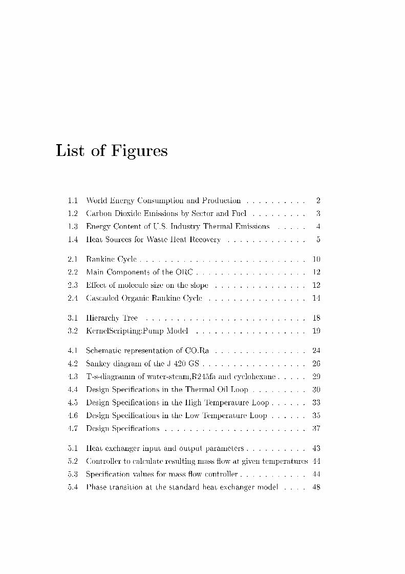
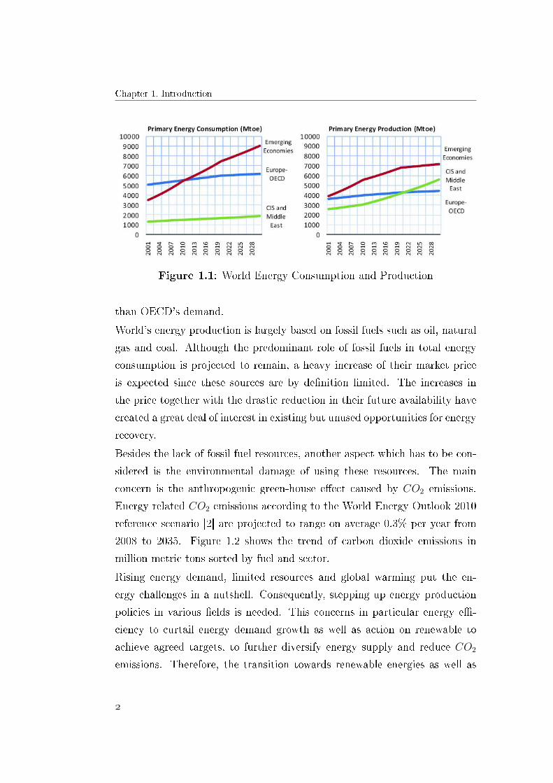
Figure 1.1 [1] depicts the projected energy consumption and production (in
million tonnes of equivalent oil) sorted by three di�erent categories: "Eu-
rope/OECD" (Europe, North America, Japan and Paci�c OECD), "Emerg-
ing Economies" (Asia, Latin America and Asia) and "CIS and Middle East",
the latter being shown as one group because they constitute the main oil and
gas producers. Both variables are given in million tonnes of equivalent oil
where one Mtoe equals 41.868 PJ. The chart shows an 11% rise in the pri-
mary energy consumption by 2030. In addition, the increasing energy needs
of emerging economies is pointed out. By 2030 they will become 45% larger
Chapter 1. Introduction
Figure 1.1: World Energy Consumption and Production
than OECD's demand.
World's energy production is largely based on fossil fuels such as oil, natural
gas and coal. Although the predominant role of fossil fuels in total energy
consumption is projected to remain, a heavy increase of their market price
is expected since these sources are by de�nition limited. The increases in
the price together with the drastic reduction in their future availability have
created a great deal of interest in existing but unused opportunities for energy
recovery.
Besides the lack of fossil fuel resources, another aspect which has to be con-
sidered is the environmental damage of using these resources. The main
concern is the anthropogenic green-house e�ect caused by CO2 emissions.
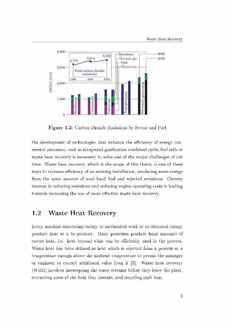
Energy related CO2 emissions according to the World Energy Outlook 2010
reference scenario [2] are projected to range on average 0.3% per year from
2008 to 2035. Figure 1.2 shows the trend of carbon dioxide emissions in
million metric tons sorted by fuel and sector.
Rising energy demand, limited resources and global warming put the en-
ergy challenges in a nutshell. Consequently, stepping up energy production
policies in various �elds is needed. This concerns in particular energy e�-
ciency to curtail energy demand growth as well as action on renewable to
achieve agreed targets, to further diversify energy supply and reduce CO2
emissions. Therefore, the transition towards renewable energies as well as
Waste Heat Recovery
Figure 1.2: Carbon Dioxide Emissions by Sector and Fuel
the development of technologies that enhance the e�ciency of energy con-
version processes, such as integrated gasi�cation combined cycle, fuel cells or
waste heat recovery is necessary to solve one of the major challenges of our
time. Waste heat recovery, which is the scope of this thesis, is one of these
ways to increase e�ciency of an existing installation, producing more energy
from the same amount of used fossil fuel and rejected emissions. Current
interest in reducing emissions and reducing engine operating costs is leading
towards increasing the use of more e�ective waste heat recovery.
1.2 Waste Heat Recovery
Every machine converting energy to mechanical work or to electrical energy
produce heat as a by-product. Many processes produce large amounts of
excess heat, i.e. heat beyond what can be e�ciently used in the process.
Waste heat has been de�ned as heat which is rejected from a process at a
temperature enough above the ambient temperature to permit the manager
or engineer to extract additional value from it [3]. Waste heat recovery
(WHR) involves intercepting the waste streams before they leave the plant,
extracting some of the heat they contain, and recycling such heat.
Chapter 1. Introduction
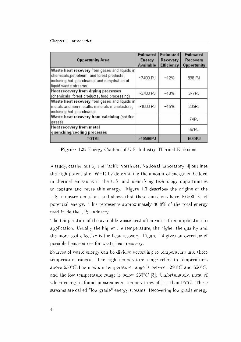
Figure 1.3: Energy Content of U.S. Industry Thermal Emissions
A study, carried out by the Paci�c Northwest National Laboratory [4] outlines
the high potential of WHR by determining the amount of energy embedded
in thermal emissions in the U.S. and identifying technology opportunities
to capture and reuse this energy. Figure 1.3 describes the origins of the
U.S. industry emissions and shows that these emissions have 10.500 PJ of
potential energy. This represents approximately 30.8% of the total energy
used in de the U.S. industry.
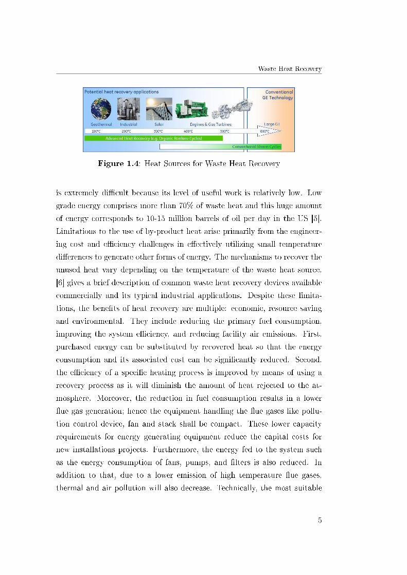
The temperature of the available waste heat often varies from application to
application. Usually the higher the temperature, the higher the quality and
the more cost e�ective is the heat recovery. Figure 1.4 gives an overview of
possible heat sources for waste heat recovery.
Sources of waste energy can be divided according to temperature into three
temperature ranges. The high temperature range refers to temperatures
above 650◦C.The medium temperature range is between 230◦C and 650◦C,
and the low temperature range is below 230◦C [3]. Unfortunately, most of
which energy is found in streams at temperatures of less than 95◦C. These
streams are called "low grade" energy streams. Recovering low grade energy
Waste Heat Recovery
Figure 1.4: Heat Sources for Waste Heat Recovery
is extremely di�cult because its level of useful work is relatively low. Low
grade energy comprises more than 70% of waste heat and this huge amount
of energy corresponds to 10-15 million barrels of oil per day in the US [5].
Limitations to the use of by-product heat arise primarily from the engineer-
ing cost and e�ciency challenges in e�ectively utilizing small temperature
di�erences to generate other forms of energy. The mechanisms to recover the
unused heat vary depending on the temperature of the waste heat source.
[6] gives a brief description of common waste heat recovery devices available
commercially and its typical industrial applications. Despite these limita-
tions, the bene�ts of heat recovery are multiple: economic, resource saving
and environmental. They include reducing the primary fuel consumption,
improving the system e�ciency, and reducing facility air emissions. First,
purchased energy can be substituted by recovered heat so that the energy
consumption and its associated cost can be signi�cantly reduced. Second,
the e�ciency of a speci�c heating process is improved by means of using a
recovery process as it will diminish the amount of heat rejected to the at-
mosphere. Moreover, the reduction in fuel consumption results in a lower
�ue gas generation; hence the equipment handling the �ue gases like pollu-
tion control device, fan and stack shall be compact. These lower capacity
requirements for energy generating equipment reduce the capital costs for
new installations projects. Furthermore, the energy fed to the system such
as the energy consumption of fans, pumps, and �lters is also reduced. In
addition to that, due to a lower emission of high temperature �ue gases,
thermal and air pollution will also decrease. Technically, the most suitable

Chapter 1. Introduction
and reliable technology for WHR is the Organic Rankine Cycle (ORC). It
is an adapted steam cycle which utilizes an organic �uid evaporating at a
lower temperature level than the water-steam phase change. Its thermody-
namic background and technical working principle will be explained in the
next chapter 2.
1.3 De�nition of Goals
The Alternative Energy Lab at GE Global Research has fully developed a
functional power plant to recover waste heat from a Jenbacher engine using a
cascaded Organic Rankine Cycle. This new cycle layout has been practised
to ensure that the maximum amount of heat is recovered at the highest
potential.
The aim of this project is to establish a thermodynamic model of the CO.Ra
product. EBSILON is the platform for the development basis of the model.
This thesis is the �rst work at GE Global Research Munich using EBSILON.
Therefore, the main scope of this work is to �nd out whether this software
is suitable or not to run ORC simulations both under design and o�-design
conditions. For this purpose, the current EBSILON component capabilities
will be studied and if needed, the standard components will be extended.
The approach to accomplish the main goal of this thesis follows next:
• De�ne the requirements for the thermodynamic model and compare
them with current EBSILON capabilities
• Extend EBSILON component models to match the simulation require-
ments
• Assemble EBSILON model of CO.Ra in design and o�-design mode
• Parametric study and sensitivity analysis of the model
The power plant to be modelled is named CO.Ra due to the cascaded ORC
technology used. It is operated by a GE Jenbacher 420 GS engine, produc-

De�nition of Goals
ing 1451 kW mechanical power at full load and working with biogas. The
CO.Ra cycle is divided in two parts, separating the recovery of two di�er-
ent temperature sources: on the one hand a high temperature loop, which
recovers the waste heat from the exhaust gas and on the other hand a low
temperature ORC, using the heat from the engine cooling water system. The
CO.Ra product has been previously modelled using HYSYS, a process sim-
ulation application developed by the company AspenTech. The design point
will be translated from HYSYS since a design optimization point was already
done by Pierre Huck in his diploma thesis [7]. The �rst step of this study is
to model and simulate the cycle under design conditions. Once the design
simulation is performed, the components will be dimensioned. Thereby a
model for their o�-design behaviour can be developed. Hence, these models
are assembled in an o�-design model of the complete cycle in order to run
the desired o�-design simulations.

Chapter 2
Technical Overview
2.1 Thermodynamic Cycles
2.1.1 Rankine Cycle
There are many di�erent approaches to transform thermal energy to elec-
tricity. One of the most e�ective energy conversion methods is the Rankine
Cycle, used in most large electric generation plants, including gas, coal, oil,
and nuclear. It is considered the ideal cycle for a simple steam power plant [8].
The Rankine Cycle based on water provides approximately 85% of worldwide
electricity production [9]. The reversible adiabatic expansion in the turbine,
the constant temperature heat rejection in the condenser, and the reversible
adiabatic compression in the pump, are similar characteristic features of both
the Rankine and the Carnot Cycles. But whereas the heat addition process
in the Rankine Cycle is reversible and at constant pressure, in the theoretical
Carnot Cycle it is reversible and isothermal. The vapour cycle is less e�cient
than the Carnot Cycle because the exhaust is completely lique�ed to facili-
tate pumping, and because superheat is added at increasing temperature[8].
These e�ects signi�cantly reduce the area of the T-s-diagram, which repre-
sents the work of the thermodynamic cycle. A basic Rankine Cycle power
plant uses a working �uid in a closed loop. Fluid is heated to its maximum
Chapter 2. Technical Overview
temperature with a heat source in a boiler or vaporizer. The high tempera-
ture and high pressure �uid is expanded in a turbine to a low pressure �uid,
where useful work is obtained, by condensing the �uid by air or water cooling
and guiding it to a tank, ready for pumping to a higher pressure where it
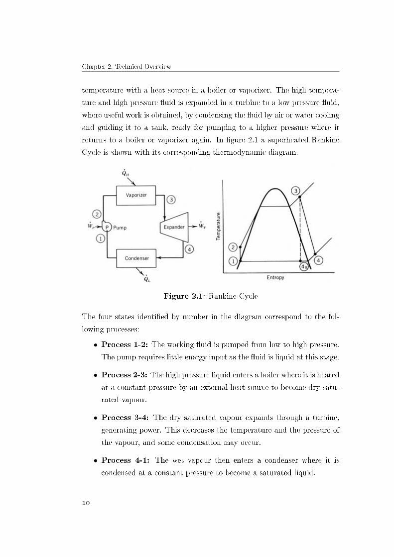
returns to a boiler or vaporizer again. In �gure 2.1 a superheated Rankine
Cycle is shown with its corresponding thermodynamic diagram.
Figure 2.1: Rankine Cycle
The four states identi�ed by number in the diagram correspond to the fol-
lowing processes:
• Process 1-2: The working �uid is pumped from low to high pressure.
The pump requires little energy input as the �uid is liquid at this stage.
• Process 2-3: The high pressure liquid enters a boiler where it is heatedat a constant pressure by an external heat source to become dry satu-
rated vapour.
• Process 3-4: The dry saturated vapour expands through a turbine,
generating power. This decreases the temperature and the pressure of
the vapour, and some condensation may occur.
• Process 4-1: The wet vapour then enters a condenser where it is
condensed at a constant pressure to become a saturated liquid.
Thermodynamic Cycles
On the T-s-diagram above, an ideal and a real expansion of the working �uid
are depicted. In a real Rankine Cycle, the compression by the pump and the
expansion in the turbine are not isotropic. These processes are non-reversible
and therefore, entropy is increased during both. Thus, the power required
by the pump increases and the power generated by the turbine decreases.
2.1.2 Organic Rankine Cycle
The principal di�erence between an installation for low-temperature heat and
conventional plants, is that in the latter water is a high satisfactory working
�uid, whereas with low temperatures, there are great advantages in using
more volatile working �uids of higher molecular weight, for example organic
�uids. The ORC process is one of the few technical options in the power
range 100 kW, which is suitable when recovering heat below 250 ◦C. This
adapted cycle works very similar to any conventional steam based Rankine
cycle. However, ORCs do not rely on high temperatures from burning fuels,
but can use much lower temperature inputs. Organic �uids, e.g. toluol or
pentan, allow heat recovery from lower temperature sources such as industrial
waste heat, geothermal heat, and solar ponds. The main di�erence between
both cycles is the lower boiling temperatures of organic �uids (compared to
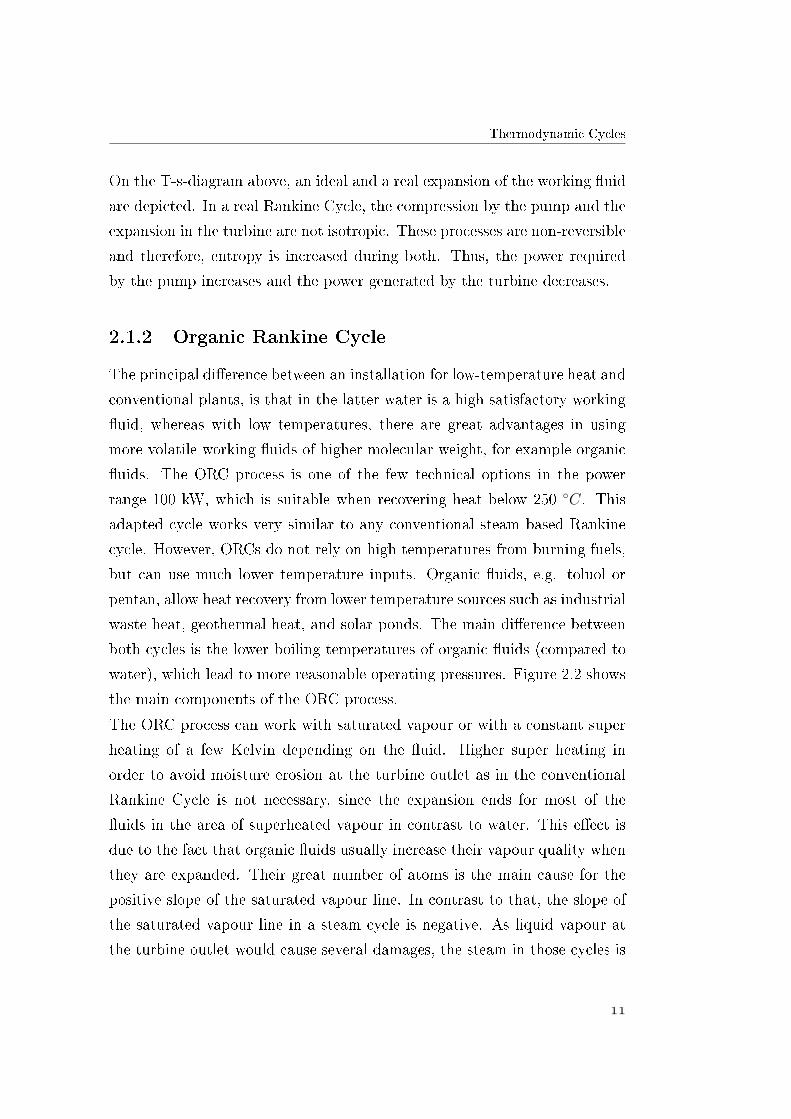
water), which lead to more reasonable operating pressures. Figure 2.2 shows
the main components of the ORC process.
The ORC process can work with saturated vapour or with a constant super
heating of a few Kelvin depending on the �uid. Higher super heating in
order to avoid moisture erosion at the turbine outlet as in the conventional
Rankine Cycle is not necessary, since the expansion ends for most of the
�uids in the area of superheated vapour in contrast to water. This e�ect is
due to the fact that organic �uids usually increase their vapour quality when
they are expanded. Their great number of atoms is the main cause for the
positive slope of the saturated vapour line. In contrast to that, the slope of
the saturated vapour line in a steam cycle is negative. As liquid vapour at
the turbine outlet would cause several damages, the steam in those cycles is
Chapter 2. Technical Overview
Figure 2.2: Main Components of the ORC
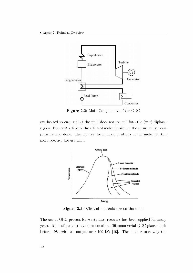
overheated to ensure that the �uid does not expand into the (wet) diphase
region. Figure 2.3 depicts the e�ect of molecule size on the saturated vapour
pressure line slope. The greater the number of atoms in the molecule, the
more positive the gradient.
Figure 2.3: E�ect of molecule size on the slope
The use of ORC process for waste heat recovery has been applied for many
years. It is estimated that there are about 30 commercial ORC plants built
before 1984 with an output over 100 kW [10]. The main reason why the
Thermodynamic Cycles
construction of new ORC plants increases is because nowadays, it can be
characterised as the only proved technology that is commonly used in ranges
of a few kW up to 1 MW [11]. However, due to the low available temperature
gradient, only very low electrical e�ciencies between 12 and 18 % are reached
[12]. Despite the fact that is linked with low e�ciencies; new applications of
this technology are commonly discussed due to its possibility to utilise the
low-level waste heat from other processes.
An overview of manufacturers together with the appropriate temperature
range of the applications is presented in [11].
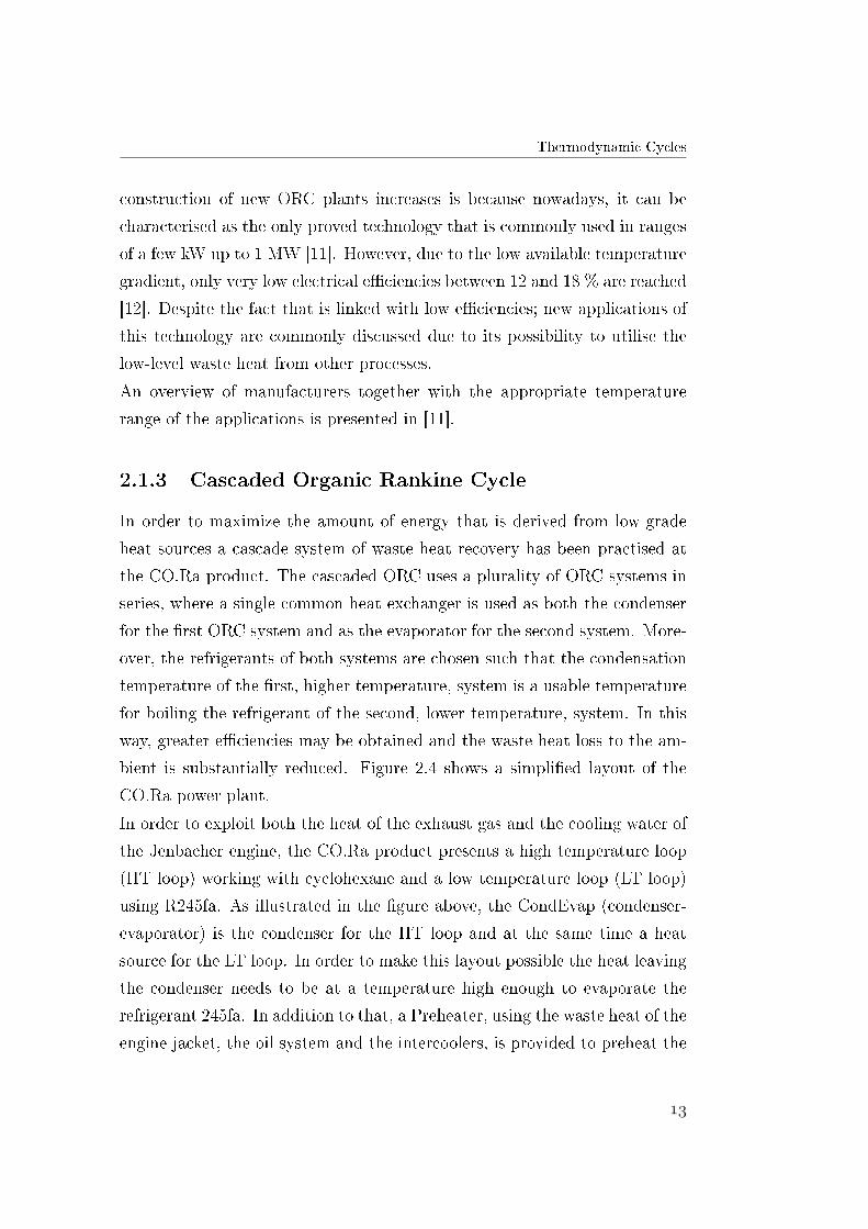
2.1.3 Cascaded Organic Rankine Cycle
In order to maximize the amount of energy that is derived from low-grade
heat sources a cascade system of waste heat recovery has been practised at
the CO.Ra product. The cascaded ORC uses a plurality of ORC systems in
series, where a single common heat exchanger is used as both the condenser
for the �rst ORC system and as the evaporator for the second system. More-
over, the refrigerants of both systems are chosen such that the condensation
temperature of the �rst, higher temperature, system is a usable temperature
for boiling the refrigerant of the second, lower temperature, system. In this
way, greater e�ciencies may be obtained and the waste heat loss to the am-
bient is substantially reduced. Figure 2.4 shows a simpli�ed layout of the
CO.Ra power plant.
In order to exploit both the heat of the exhaust gas and the cooling water of
the Jenbacher engine, the CO.Ra product presents a high temperature loop
(HT loop) working with cyclohexane and a low temperature loop (LT loop)
using R245fa. As illustrated in the �gure above, the CondEvap (condenser-
evaporator) is the condenser for the HT loop and at the same time a heat
source for the LT loop. In order to make this layout possible the heat leaving
the condenser needs to be at a temperature high enough to evaporate the
refrigerant 245fa. In addition to that, a Preheater, using the waste heat of the
engine jacket, the oil system and the intercoolers, is provided to preheat the

Chapter 2. Technical Overview
Figure 2.4: Cascaded Organic Rankine Cycle
working �uid in the second ORC system prior to its entry into the common
heat exchanger. Waste heat streams are typically in the form of hot liquid
or gas. This heat is transferred to the ORC working �uid, either directly (
direct exchange between waste heat and working �uid) or indirectly (with an
intermediate medium closed loop) depending upon the characteristics of the
waste heat source and other constraints. Typically, waste heat liquid �ows are
directly coupled to the ORC cycle, while gas �ows are indirectly coupled [13].
In the CO.Ra case, an indirect heat recovery scheme is employed, the heat
source exchanges heat with thermal oil building the TO loop, and afterwards
feeds the ORC cycle.
This cycle layout takes much better advantage of the availability of two
separate heat sources than it could be achieved with two heat engines, each
operating from its own source. Because of the use of these common heat
exchangers, heat is being cascaded from HT loop to LT loop so that a high
power output at low speci�c cost is obtained. Moreover, the cascaded Organic

O�-Design Background
Rankine Cycle presents a lower speci�c enthalpy drop over the turbine, which
permits a reasonable operating pressure. The CO.Ra plant layout and its
components will be described in detail in chapter 4.
2.2 O�-Design Background
Every power plant is subjected to di�erent operation and maintenance sched-
ules so that the plant operates in conditions di�erent from those given at full
output power. An o�-design case can be de�ned as a case, for which the heat
input or the heat removal in the considered thermodynamic cycle is not equal
to the one at the design point. H. Gurgenci describes o� design operation as
the operation at temperatures di�erent from the design point temperatures
and at varying loads (+/- 50%) [14].
In most ORC applications, in contrast to conventional power plants, the
o�-design operation could be actually the normal mode of operation. For
instance, when recovering industrial waste heat recovery, the temperature of
the waste heat stream may steadily vary. However, the goal of the plant
modelled in this work is to run it at base load for the majority of the time
but as part of an overall grid strategy part load operation will also come into
play. As mentioned in chapter 1.3, the topic of this study is the analysis of a
cascaded ORC power plant, with a special focus on the o�-design behaviour
of the di�erent components. In order to perform realistic o�-design models,
the model has to be �rst simulated under design conditions. Once the heat
and mass balances at on-design conditions have been evaluated, one can
calculate the relevant non-dimensional parameters of the components,e.g.
the products (U· A) of each heat exchanger, where U is the overall heat
transfer coe�cient and A is the heat transfer area. After the components of
the cycle have been dimensioned, o�-design simulations can be performed.
It should be mentioned that o�-design conditions can a�ect the design of the
process. Taking into account the o�-design cases is therefore very important
during the design e�orts. Heat and mass balances and performances at o�-

Chapter 2. Technical Overview
design conditions are estimated by accounting for the constraints imposed
by the available heat transfer areas in heaters and condensers, as well as the
characteristic curves of pumps and turbines [15].
The focus of the steady-state o�-design simulations carried out in this study
is on the one hand, the sensitivity analysis of the simulation model and on
the other hand the calculation of the rotary speed of pumps and expanders
in order to operate the plant close to the design point. Here the sensitivity
analysis will be used to evaluate the e�ect of the model input data uncertainty
on the simulation results. The aim of such analysis is to show, which are
the most sensitive result values for input parameter variations and which
input parameters have the greatest e�ect on the results. This thesis will
�rst focus on modelling the plant under design conditions. The de�nition of
an optimized design point has already been done by Huck in [7] using the
simulation software Aspen One HYSYS. Hence, inputs such as the turbine
design point and the pump design point or the degree of overheating and sub
cooling will be linked in from the HYSYS CO.Ra design model. A detailed
description of the design conditions is given in chapter 4. After the design
model of the process has been created, the components will be modelled
according to the speci�cations of the manufacturer. In case of the pumps,
for example, the characteristic curves provided by the supplier will describe
the o�-design behaviour of the pump at di�erent speed inputs. Models to
describe pump, expander, heat exchanger and valves performance in o�-
design operation and the way they have been implemented will be outlined
in chapter 5.
Chapter 3
Used Software:EBSILON
3.1 Main Features
The software used in this thesis to run thermodynamic calculation on the
di�erent cycle conditions is EBSILON, a process simulation application de-
veloped by the company Evonik. EBSILON is the abbreviation for "Energy
balance and simulation of the load response of power generating or process
controlling network structures" and it is used for all kind of power plants and
thermodynamic processes. EBSILON is basically composed of two global cal-
culation modes:
• Design Calculation ("full load")
• O�-design Calculation ("part load")
The design mode is used for the construction of new cycles. In this mode, the
user de�nes appropriate values for all components, e.g. according to speci�-
cations from manufacturer. The cycle is simulated under design conditions,
which are, for example, the engine running at full load or 15 ◦C ambient
temperature. The results of the design calculations are stored as reference
values for o�-design and allow the components to be dimensioned. In o�-
design mode components are then �xed and simulations can be performed
for di�erent variations (di�erent sets of input data). As already mentioned
Chapter 3. Used Software:EBSILON
in chapter 2.2, o�-design corresponds to the operating conditions which vary
from the nominal point, e.g. the engine running at partial load.
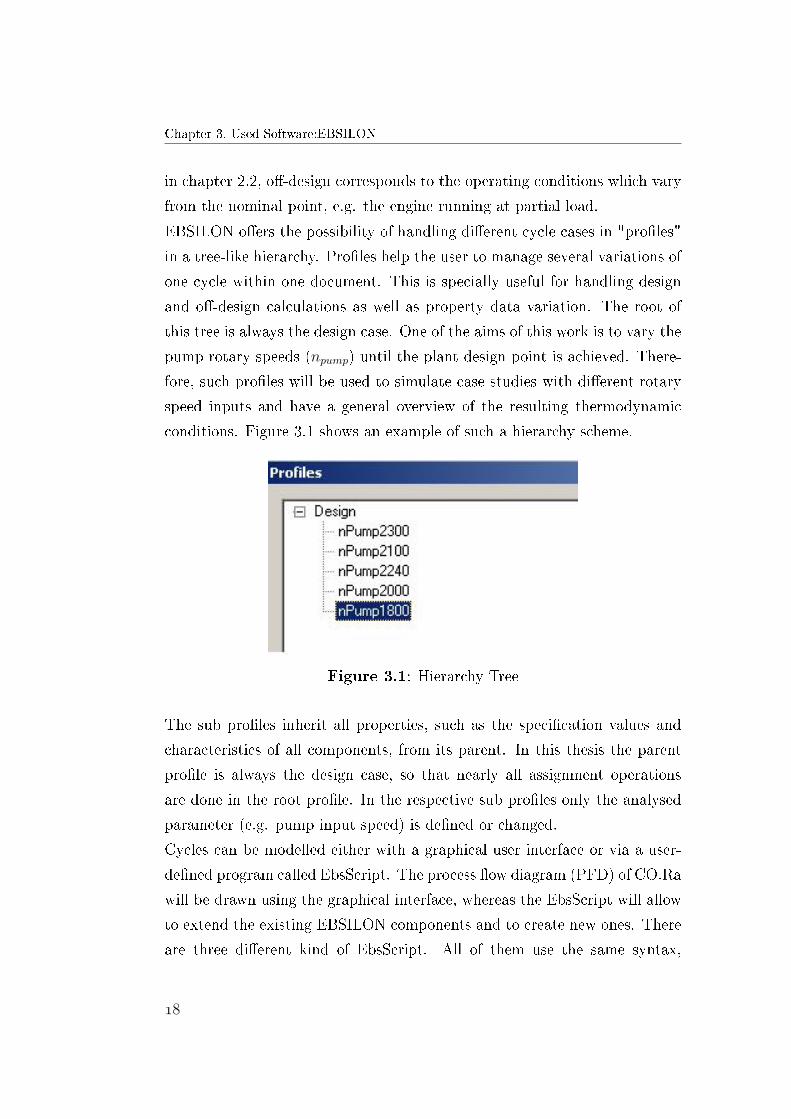
EBSILON o�ers the possibility of handling di�erent cycle cases in "pro�les"
in a tree-like hierarchy. Pro�les help the user to manage several variations of
one cycle within one document. This is specially useful for handling design
and o�-design calculations as well as property data variation. The root of
this tree is always the design case. One of the aims of this work is to vary the
pump rotary speeds (npump) until the plant design point is achieved. There-
fore, such pro�les will be used to simulate case studies with di�erent rotary
speed inputs and have a general overview of the resulting thermodynamic
conditions. Figure 3.1 shows an example of such a hierarchy scheme.
Figure 3.1: Hierarchy Tree
The sub pro�les inherit all properties, such as the speci�cation values and
characteristics of all components, from its parent. In this thesis the parent
pro�le is always the design case, so that nearly all assignment operations
are done in the root pro�le. In the respective sub pro�les only the analysed
parameter (e.g. pump input speed) is de�ned or changed.
Cycles can be modelled either with a graphical user interface or via a user-
de�ned program called EbsScript. The process �ow diagram (PFD) of CO.Ra
will be drawn using the graphical interface, whereas the EbsScript will allow
to extend the existing EBSILON components and to create new ones. There
are three di�erent kind of EbsScript. All of them use the same syntax,
Main Features
i.e. Pascal, and enable the user to use the input, output and calculation
capabilities of EBSILON in an automatic way. However, they are used for
di�erent purposes.
A complete model can be created and simulated with the "general" EbsSript.
Here the user can use commands such as "simulate" or "validate". EbsScript
is suitable for parameter variation studies. An other interesting feature is
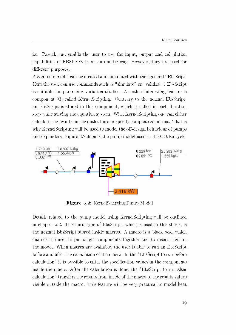
component 93, called KernelScripting. Contrary to the normal EbsScript,
an EbsScript is stored in this component, which is called in each iteration
step while solving the equation system. With KernelScripting one can either
calculate the results on the outlet lines or specify complete equations. That is
why KernelScripting will be used to model the o�-design behaviour of pumps
and expanders. Figure 3.2 depicts the pump model used in the CO.Ra cycle.
Figure 3.2: KernelScripting:Pump Model
Details related to the pump model using KernelScripting will be outlined
in chapter 5.2. The third type of EbsScript, which is used in this thesis, is
the normal EbsScript stored inside macros. A macro is a black box, which
enables the user to put single components together and to insert them in
the model. When macros are available, the user is able to run an EbsScript
before and after the calculation of the macro. In the "EbsScript to run before
calculation" it is possible to enter the speci�cation values in the components
inside the macro. After the calculation is done, the "EbsScript to run after
calculation" transfers the results from inside of the macro to the results values
visible outside the macro. This feature will be very practical to model heat
Chapter 3. Used Software:EBSILON
exchangers. A detailed explanation is given in chapter 5.1.
The main di�erence between these three kinds of scripts is that by using
the normal EbsScript or the script inside the macros, neither the EbsScript
nor the user can access the calculation. The control is given back to the
EbsScript after the calculation has �nished. On the contrary, with the help of
component 93 it is possible to have direct access in the course of calculation.
3.2 Comparison of EBSILON and HYSYS
As mentioned in section 1.3, a steady-state thermodynamic model of the
CO.Ra product has been previously done using HYSYS. This thesis is the
�rst work at GRC employing EBSILON. Hence, a comparison regarding the
capabilities of both software will be drawn next. This section aims to give
an overview of the pros and cons of each software regarding the purpose of
this thesis.
The �rst and most distinctive feature, which makes EBSILON suitable for
this thesis is its dedicated o�-design calculation mode and the possibility of
handling di�erent cases in pro�les. The user is able to run o�-design sim-
ulations by just switching the calculation mode (from design to o�-design)
in the di�erent pro�les so that the calculation is then performed according
to the o�-design rules. On the contrary, HYSYS has neither the o�-design
calculation mode nor the pro�le hierarchy tree. O�-design simulations can be
performed by using a logical operator called "Adjust", which permits to set
a calculated parameter to a target numerical value, by changing a speci�ed
parameter. For instance, setting the overall heat transfer coe�cient of a HX
to a �x value and calculate a resulting temperature in the cycle. An example
of the use of this feature can be found in [7]. However, this way of simulating
the o�-design behaviour of the power plant is less numerically stable. First of
all, the user has to continuously modify the basis model by building several
"Adjust" operators. That means, that if it does not converge the basis model
has to be �xed. Moreover, performing o�-design simulations in HYSYS re-
Comparison of EBSILON and HYSYS
quires an expert user, since the behaviour of such logical operators has to be
controlled during the calculation. The user will have to enable and disable
them at di�erent times to help the system to converge. In other words, in
HYSYS it is not possible to run o�-design simulation in an automatic and
easy way. Similar to the pro�le feature in EBSILON, in HYSYS one is able
to run its own calculation of the system by using a spreadsheet, which is in-
tegrated in the simulation. Here the user can simulate di�erent case studies.
However, when it comes to perform parameter studies at relative complex
models, the use of a spreadsheet hinders the convergence.
Another important aspect is the manner how independent components can
be implemented in both software. One of the goals of this thesis is to ex-
tend the EBSILON component models to match the simulation requirements.
Therefore, complex equations will have to be implemented for the di�er-
ent components. Whereas in EBSILON components can be extended using
KernelScripting, in HYSYS the use of the spreadsheet also allows to de�ne
its own components and to include them in the simulation. Nevertheless,
the implementation using a spreadsheet is quite limited, since its capaci-
ties are comparable to the ones of an excel sheet. HYSYS spreadsheet can
only process available components outputs (add, subtract) and write them in
available component inputs. One can not implement, for instance, quadratic
functions/dependencies or iterative loops. This constraint does not allow, for
instance, the implementation of an empirical model, like it will be done in
the case of the expander (see chapter 5.3). Another di�erence between both
simulation software is the �uid properties used. EBSILON uses the REF-
PROP library, whereas HYSYS calculates with the Zudkevitch-Jo�ee �uid
package. Implementing the REFPROP properties in HYSYS increments the
computational cost of the simulations. Comparing the capabilities of the
standard heat exchanger model in both software, in HYSYS, it already ex-
ists a weighted heat exchanger design where the user is able to specify the
number of intervals for each pass in the HX. This design applies to non-linear
heat curve problems such as the phase change of pure components. Heating

Chapter 3. Used Software:EBSILON
curves are broken into intervals and an energy balance is performed along
each interval. In EBSILON the standard HX treats the heat curves for both
heat exchanger sides as linear, so that a constant overall heat transfer coef-
�cient (U) is assumed. Consequently, the phase change of the working �uid
is not considered properly, which results in an incorrect calculated LMTD
value. In order to solve this issue, a multi-cell heat exchanger model will be
developed in EBSILON. Further details will be given in chapter 5.1.
Comparing the mentioned characteristics, both software present its advan-
tages and disadvantages. Whereas HYSYS is mainly used in the oil and gas
industry, EBSILON is specially designed for simulating power plants and
thermodynamic processes. The integrated o�-design solver and the user de-
�ned script are the main features which motivated to start to use EBSILON
to run ORC simulations.

Chapter 4
Plant Design
As mentioned before the main purpose of CO.Ra is to recover waste heat
from a GE Jenbacher gas engine to produce additional electrical power. This
chapter focuses on the technical features of the engine, the description of
the cycle layout and on the selected working �uid properties. Moreover, the
CO.Ra cycle design point will be presented as well as its implementation in
EBSILON. Figure 4.1 gives a schematic representation of the cascaded plant
layout.
The cycle is divided in two parts: on the one hand, a high temperature
ORC utilizing heat from the exhaust gas stream and on the other hand, a
low temperature ORC, recovering heat from the engine cooling water system.
Further, the heat from the exhaust gas is transferred to the HT loop by means
of an intermediate thermal oil loop. The loops are arranged in a cascaded
way to use the condensation heat from the high temperature cycle and use
it for evaporation in the low temperature cycle.
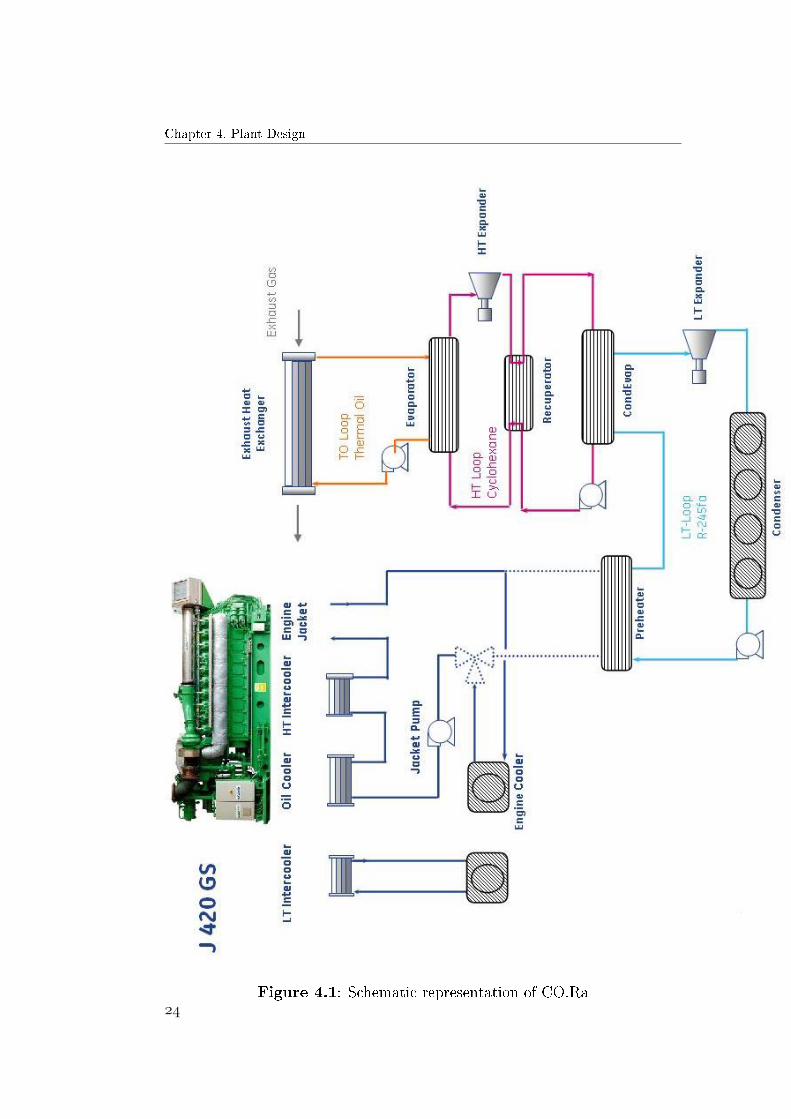
Chapter 4. Plant Design
Figure 4.1: Schematic representation of CO.Ra

Heat Source
4.1 Heat Source
The type of engine considered in this work is the J 420 GS from GE Jen-
bacher. The engine, producing 1451 kW mechanical power at full load is
part of the low power engine portfolio of GE Jenbacher. It is a 20 cylinder,
4-stroke Otto-engine, driven with biogas. Organic substances like food waste
and maize silage are fermented by bacteria, producing biogas. However, the
engine can be fuelled with di�erent sorts of gas such as natural-, land�ll-
and coalmine-gas. An overview of the most important engine data is given
in Table 4.1.
Table 4.1: Data of the GE Jenbacher engine J420 GS
Description Data
Con�guration 20 cylinder in-lineWorking Principle Spark-ignition engine
Gas types Natural gas, special gasesGas power Input 3480 kW
Electrical Power Output 1415 kWElectrical E�ciency 40.60%
The engine is supplied with gas equivalent to a power of 3840 kW. From
this work input, in form of thermal energy of the combustion, 1451 kW are
converted into mechanical power. This results in a thermal e�ciency of the
engine of 41.7 %. Assuming a generator e�ciency of 97.5 % gives a �nal
electrical e�ciency of about 40.6 %. According to this value an electrical net
output power of 1415 kW is obtained. Without any additional measures the
rest of the heat, i.e 2425 kW, is discarded to the ambient. Despite the fact,
that the waste heat provided by the engine cannot be entirely recovered due
to physical limitations, it's potential is still very interesting. The detailed
distribution of the energy �ow for nominal conditions as well as the amount
of waste heat, which can be e�ectively recovered, is depicted in the Sankey
diagram in �gure 4.2.

Chapter 4. Plant Design
Figure 4.2: Sankey diagram of the J 420 GS
The J420 has four important waste heat sources, namely the cooling wa-
ter (CW), the inter cooler, the oil lubrication system and the exhaust gas
stream. Heat at a temperature of about 90 ◦C is available from the �rst three
subsystems. These can be classi�ed as the low temperature heat source and
represent ca. 23% of the heat input. On the other hand, around 600 kW are
available if the exhaust gases are cooled from 427 ◦C to 180 ◦C. This amount
of heat accounts for 17% of the heat input and for 25% of the total waste
heat in the present con�guration. Altogether, 1390 kW of heat are used to
operate the CO.Ra cycle. Because of the di�erent temperature level of the
heat sources two di�erent �uids have been selected in order to pro�t both
of them with the maximum e�ciency. The criteria for the �uid selection are
outlined in the following section.

Working Fluid Properties
4.2 Working Fluid Properties
The selection of the working �uid is of key importance in low temperature
Rankine Cycles. As mentioned in chapter 2.1.3 the main aim when deciding
the cycle layout is to improve the e�ciency as much as possible. The highest
achievable e�ciency depends strongly on the thermodynamic characteristics
of the �uid and on the operating conditions. Before determining the optimum
thermodynamic quantities of the process, a suitable working �uid has to be
selected. Possible working media for ORC plants are all �uids that have their
boiling temperature at reasonable pressures in the demanded temperature
range between the maximum temperature (energy source) and the minimum
one (energy sink or cooling). In recent years, di�erent media have been
proposed and also utilized. However, refrigerants and hydrocarbons are the
two commonly used components in order to recover low-grade waste heat.
Dry �uids show better thermal e�ciencies because they do not condense after
the �uid goes through the turbine as opposed to wet �uids that produce
condensates after the turbine [16]. In order to identify the most suitable
organic �uids, several general criteria have to be taken into consideration,
including [17]:
• Thermodynamic properties
• Stability of the �uid and compatibility with materials in contact
• Safety, health and environmental aspects
• Availability and costs
To recover both the heat of the exhaust gas stream and the engine cooling
water system, cyclohexane and R245fa have been chosen among other or-
ganic �uids and refrigerants according to prior GE Global Research studies,
focusing on costs and performance analysis [18]. The results of calculation
of theoretical e�ciency and power of Rankine cycle for di�erent refrigerants
are presented in [19]. The most important properties to be considered are
listed in table 4.2 at standard conditions for temperature and pressure [20].

Chapter 4. Plant Design
Table 4.2: Selected Properties of Cyclohexane and R245fa
Description Data Cyclohexane Data R245fa
Speci�c Heat 1.728 J / (kg·K) 1.301 J/ (kg·K)Enthalpy of Vaporization 356 J/ kg 196 J/ kg
Density 783.4 kg/m3 1320 kg/m3
Boiling Point 80.7 ◦C 15.3 ◦CMelting Point 6.54 ◦C −103 ◦CFluid Type Dry Dry
Organic �uids usually su�er chemical deteriorations and decomposition at
high temperatures. The maximum hot temperature is thus limited by the
chemical stability of the working �uid. On the other hand, the freezing point
of both working �uids should be lower than the ambient temperature, so that
in winter no freezing of the working �uid occurs once the plant is not run-
ning. This aspect is especially important in the HT loop, since cyclohexane
freezes at 1 bar pressure and 6.5 ◦C. In order to keep the temperature inside
the container above the freezing limit electrical heaters have been installed.
Cyclohexane is a saturated cyclic hydrocarbon without halogens. This work-
ing �uid is harmful, highly in�ammable and hazardous to health. It is mostly
used in chemical industry as solvent and for producing plastics. With an ig-
nition temperature of 245◦C, appropriate measures have to be taken in order
to ensure a safe operation of the plant when recovering the heat from the
exhaust gas stream. These are discussed in the following section.
Unlike cyclohexane, R245fa is not classi�ed as a hazardous substance. It is
mostly used for cooling applications or for producing foam. Viewed chemi-
cally, it is a hydro �uorocarbon. It is not �ammable and so the hazardous
potential is low. Moreover, the boiling point of R45fa is lower than the one
of cyclohexane, making it suitable for the LT loop.
As described in table 4.2 the selected �uids have a low enthalpy of vapor-
ization. With increasing speci�c enthalpy of vaporization the slope of the
saturated vapour curve decreases. Substances that form hydrogen bonds
such as water, ammonia or ethanol have a comparatively large enthalpy of
Working Fluid Properties
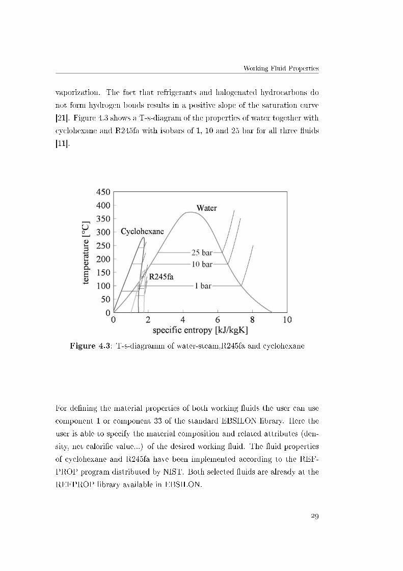
vaporization. The fact that refrigerants and halogenated hydrocarbons do
not form hydrogen bonds results in a positive slope of the saturation curve
[21]. Figure 4.3 shows a T-s-diagram of the properties of water together with
cyclohexane and R245fa with isobars of 1, 10 and 25 bar for all three �uids
[11].
Figure 4.3: T-s-diagramm of water-steam,R245fa and cyclohexane
For de�ning the material properties of both working �uids the user can use
component 1 or component 33 of the standard EBSILON library. Here the
user is able to specify the material composition and related attributes (den-
sity, net calori�c value,..) of the desired working �uid. The �uid properties
of cyclohexane and R245fa have been implemented according to the REF-
PROP program distributed by NIST. Both selected �uids are already at the
REFPROP library available in EBSILON.
Chapter 4. Plant Design
4.3 Plant Description
4.3.1 Thermal Oil Loop
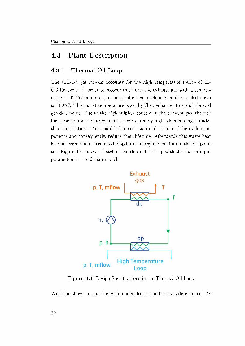
The exhaust gas stream accounts for the high temperature source of the
CO.Ra cycle. In order to recover this heat, the exhaust gas with a temper-
ature of 427◦C enters a shell and tube heat exchanger and is cooled down
to 180◦C. This outlet temperature is set by GE Jenbacher to avoid the acid
gas dew point. Due to the high sulphur content in the exhaust gas, the risk
for these compounds to condense is considerably high when cooling it under
this temperature. This could led to corrosion and erosion of the cycle com-
ponents and consequently, reduce their lifetime. Afterwards this waste heat
is transferred via a thermal oil loop into the organic medium in the Evapora-
tor. Figure 4.4 shows a sketch of the thermal oil loop with the chosen input
parameters in the design model.
Figure 4.4: Design Speci�cations in the Thermal Oil Loop
With the shown inputs the cycle under design conditions is determined. As
Plant Description
the pressure drop in the heat exchangers is known, also the pressures after
the HX are known. In this mode the user needs to de�ne three temperatures
and the mass �ow at each HX so that the outlet temperature and the required
nominal heat transfer coe�cient is calculated.
However, in the case of the exhaust heat exchanger, all four temperatures are
de�ned in order to obtain the mass �ow of the thermal oil loop as a result.
Adding a controller at the HX outlet, the mass �ow is modi�ed until the
target value for the temperature is achieved. A detailed explanation of this
modelling issue is given in chapter 5.1.
The pump is de�ned by specifying the enthalpy and the pressure at the inlet
as well as its e�ciency. A table summarizing the assumed e�ciencies for
pumps and expanders at the nominal point can be found at the end of this
chapter.
The oil used in this intermediate loop is Therminol 59; a synthetic heat
transfer �uid with excellent thermal stability and low viscosity. This kind
thermal oil is not present in the EBSILON components library. However, the
user can specify the data of the desired thermo liquid by himself. In order
to implement Therminol 59 following coe�cients have been introduced.
• the molar weight (M=100kg/kmol)
• the extents of validity for temperature, enthalpy, and entropy
• the coe�cients for calculating the speci�c heat cp
cp = 1.6175 + 3.2 · 10−3 · T + 5 · 10−7 · T 2 (4.1)
• the coe�cients for calculating the density ρ (in kg/m3):
ρ = 988.31− 0.6951 · T − 3 · 10−4 · T 2 (4.2)
The coe�cients for the speci�c heat capacity and the density have been cal-
culated with the data provided by the supplier. These data can be found

Chapter 4. Plant Design
at the Appendix (A.2). Optionally coe�cients for the heat conductivity, the
dynamic and kinematic viscosity as well as for the enthalpy and the entropy
can be speci�ed. The speci�cation of these latter values (enthalpy and en-
tropy) serves to decrease the computing time as EBSILON uses the quantities
calculated from these polynomials as initial value.
The use of this TO loop has from a thermodynamic as well as from a �nancial
point of view several drawbacks. Building this intermediate loop increases
the number of components to be installed, which results in a higher cost of
the plant. Moreover, heat losses also rise due to increased piping.
Even so, the TO loop has to be build for safety reasons. As stated in sec-
tion 4.2, organic �uids might deteriorate at high temperatures. Since the
exhaust gas temperature is approximately 425◦C, the chemical stability of
cyclohexane has to be considered. This �uid should not be heated to more
than 300◦C. Besides that, contrary to R245fa, cyclohexane is a �ammable
substance, so that its direct evaporation by the exhaust gas could led to to
ignition in case of leakage.
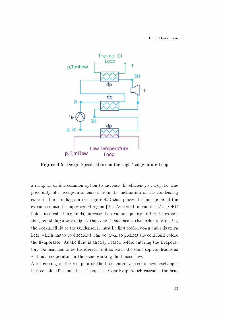
4.3.2 High Temperature Loop
Figure 4.5 depicts the HT loop of the CO.Ra layout in a simpli�ed way.
Once the heat of the thermal oil is transferred to the HT loop via the Evapora-
tor, cyclohexane is evaporated and superheated by 10 K at the nominal point.
This superheat must be high enough to avoid droplets at the expander inlet,
although the maximum cycle e�ciency would be obtained without super-
heating. Moreover, the expander inlet temperature can not exceed 180◦C,
since the �ow exiting the impeller is used to cool the generator. This gener-
ator constitutes the �rst power source of the cycle concept, obtaining a net
electrical power output of approximately 60 kW under design conditions.
The cyclohexane expands in a radial turbine reaching a superheat degree
of nearly 42 K. Afterwards, the working �uid �ows to a recuperator. Here
the dry vapour is de-superheated before entering the condenser whereas the
liquid cyclohexane is preheated before entering the Evaporator. The use of
Plant Description
Figure 4.5: Design Speci�cations in the High Temperature Loop
a recuperator is a common option to increase the e�ciency of a cycle. The
possibility of a recuperator ensues from the inclination of the condensing
curve in the T-s-diagram (see �gure 4.3) that places the �nal point of the
expansion into the superheated region [19]. As stated in chapter 2.1.2, ORC
�uids, also called dry �uids, increase their vapour quality during the expan-
sion, remaining always higher than one. That means that prior to directing
the working �uid to the condenser it must be �rst cooled down and this extra
heat, which has to be discarded, can be given to preheat the cold �uid before
the Evaporator. As the �uid is already heated before entering the Evapora-
tor, less heat has to be transferred to it to reach the same top conditions as
without recuperator for the same working �uid mass �ow.
After cooling in the recuperator the �uid enters a second heat exchanger
between the HT- and the LT loop, the CondEvap, which cascades the heat

Chapter 4. Plant Design
of the condensation of the HT working �uid to the low temperature ORC.
At the outlet of the CondEvap the bottom temperature of the HT loop is
reached with around 10 K of subcooling.
In order to de�ne the expander in design mode, the user needs to implement
the same inputs as for the pump (e�ciency, pressure at inlet and outlet and
enthalpy at inlet). Notice that in this case the enthalpy at the inlet of the
pump is given by the sub-cooling (SC) after the CondEvap, whereas the en-
thalpy at the expander inlet is de�ned with the superheat (SH) of the �uid.
Similar to the thermal oil loop, the mass �ow of the HT loop is regulated by
means of a controller with the degree of superheat at the recuperator outlet.
The pressure increase in this loop has been speci�ed by giving the pressure
at the inlet and the outlet of the pump.
4.3.3 Low Temperature Loop
As mentioned in section 4.2, the refrigerant R245fa has been used to re-
cover the heat from the engine cooling water system. The low temperature
heat sources (jacket water, lubrication system and intercooler) are directly
included into the low temperature loop, being exploited in a brazed plate
heat exchanger called Preheater. Here, the refrigerant is being preheated
and partially evaporated before entering the CondEvap. The LT loop is de-
signed similar to the HT cycle. Figure 4.6 shows the thermal �ow diagram
of the low temperature loop.
Concerning the �uid composition, typically 40 % Mass glycol can be added
to the jacket water as an anti-freezing measure. The speci�c heat capacity
(cp) for the Water-Glycol mixture can be calculated in the following way:
cp = 4.192 · (1− Glycolfraction
100) + 2.97 · Glycolfraction
100(4.3)
With the speci�ed mass fraction, a cp of 3.71 kJ/kg· K is obtained. The Pre-
heater, as the interface between the engine cooling system and the CO.Ra
cycle, recovers the large quantity of lower temperature waste heat and pre-
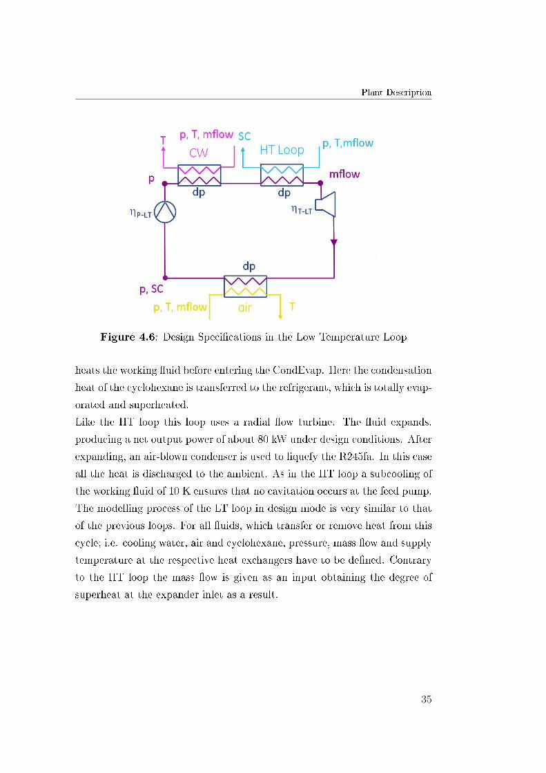
Plant Description
Figure 4.6: Design Speci�cations in the Low Temperature Loop
heats the working �uid before entering the CondEvap. Here the condensation
heat of the cyclohexane is transferred to the refrigerant, which is totally evap-
orated and superheated.
Like the HT loop this loop uses a radial �ow turbine. The �uid expands,
producing a net output power of about 80 kW under design conditions. After
expanding, an air-blown condenser is used to liquefy the R245fa. In this case
all the heat is discharged to the ambient. As in the HT loop a subcooling of
the working �uid of 10 K ensures that no cavitation occurs at the feed pump.
The modelling process of the LT loop in design mode is very similar to that
of the previous loops. For all �uids, which transfer or remove heat from this
cycle; i.e. cooling water, air and cyclohexane, pressure, mass �ow and supply
temperature at the respective heat exchangers have to be de�ned. Contrary
to the HT loop the mass �ow is given as an input obtaining the degree of
superheat at the expander inlet as a result.

Chapter 4. Plant Design
4.4 Design Point
The o�-design behaviour of a thermodynamic model can not be evaluated
without knowing its design point. Hence, this thesis has �rst focused on
modelling the CO.Ra cycle at the design point. As mentioned before, a design
point optimization was already done by Huck in [7] using HYSYS. Therefore,
the values for the chosen design inputs will be translated from the existing
HYSYS model. Based on the results of the design simulation the di�erent
components of the cycle are dimensioned. Once the input variables for each
loop have been decided, the cycles can be assembled so that simulations with
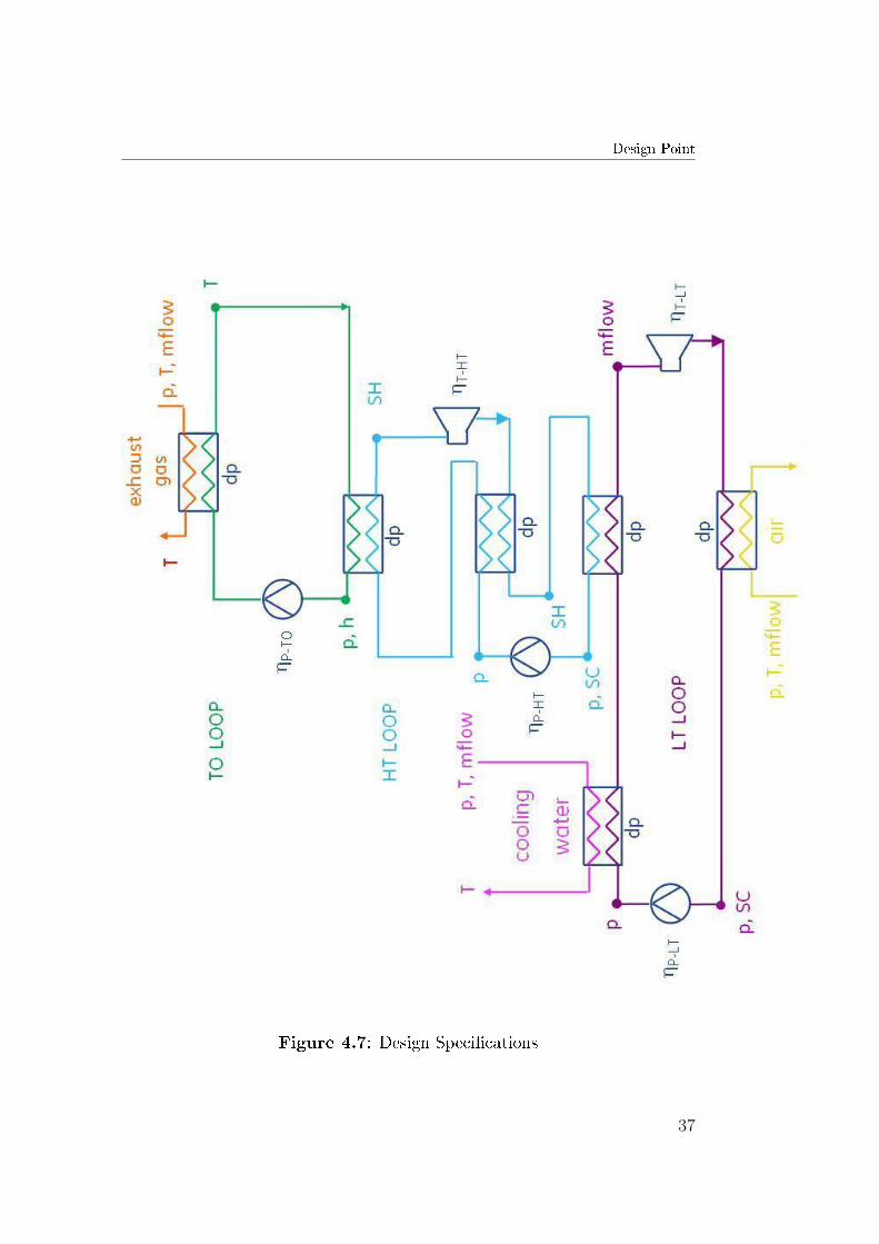
an integrated model of the whole installation can be performed. Figure 4.7
illustrates the con�guration and the chosen inputs for the model in design
mode.
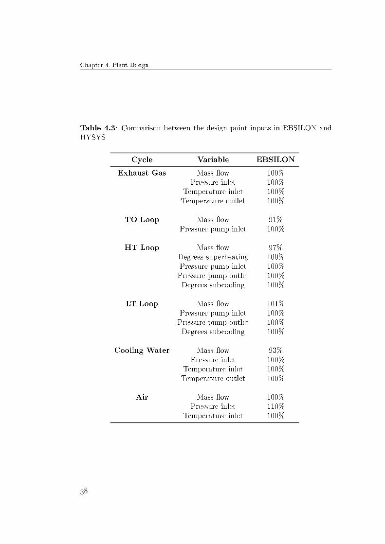
Table 4.3 gives a comparison between the on-design operating conditions
assumed for the CO.Ra power plant and the existing HYSYS design model.
The depicted values have been normalized with the values de�ned in HYSYS
(100% means that the variable has got the same value in both simulation
software). Almost all input parameters have been exactly de�ned as in the
HYSYS model. Only the mass �ow values at the three loops di�er. This
variation has to do with the fact that whether the �uid properties nor the
same component inputs have been used. Moreover, the assumed e�ciencies
at the nominal point are not equal.
As mentioned in section 4.2, EBSILON uses the REFPROP library for both
organic �uids. On the other hand, HYSYS calculates with the Zudkevitch-
Jo�ee �uid package. The main assumptions adopted regarding the pump and
expander e�ciencies to estimate the on-design heat and mass balances and
the performances of the power plant are shown in table 4.4. The e�ciencies at
the design point have been calculated in the following way. First, the pumps
and expanders rotary speeds in order to run the plant close to the design
point have been found simulating the model under o�-design conditions (see
chapter 7.2). After, these speed values have been introduced at the o�-
design pump and expander model. Finally, the e�ciencies obtained using
Design Point
Figure 4.7: Design Speci�cations
Chapter 4. Plant Design
Table 4.3: Comparison between the design point inputs in EBSILON andHYSYS
Cycle Variable EBSILON
Exhaust Gas Mass �ow 100%Pressure inlet 100%
Temperature inlet 100%Temperature outlet 100%
TO Loop Mass �ow 91%Pressure pump inlet 100%
HT Loop Mass �ow 97%Degrees superheating 100%Pressure pump inlet 100%Pressure pump outlet 100%Degrees subcooling 100%
LT Loop Mass �ow 101%Pressure pump inlet 100%Pressure pump outlet 100%Degrees subcooling 100%
Cooling Water Mass �ow 93%Pressure inlet 100%
Temperature inlet 100%Temperature outlet 100%
Air Mass �ow 100%Pressure inlet 110%
Temperature inlet 100%

Design Point
these models have been set at the design point. Both pump and expander
o�-design models are explained in the next chapter.
Table 4.4: Realistic hypotheses for pump and expander e�ciencies
Cycle Variable EBSILON HYSYS
TO Loop Thermal oil pump e�ciency 60 % 60 %
HT Loop Cyclohexane pump e�ciency 64 % 50 %Cyclohexane expander e�ciency 90 % 82 %
LT Loop R245fa pump e�ciency 73 % 50 %R245fa expander e�ciency 72 % 82 %

Chapter 5
Extended Component Models
The �rst step to establish the thermodynamic model of CO.Ra is to analyse
the existing HYSYS model in order to study the used components. Once
both the input and output parameters at each component are identi�ed, a
comparison with the current EBSILON component capabilities has to be
drawn. This chapter presents the modi�cations carried out at the standard
EBSILON components to match the simulation requirements. A description
of the main issues which came up by modelling heat exchangers, pumps and
expanders as well as the equations and variables used in the respective models
follows next.
5.1 Heat Exchanger Model
5.1.1 Technical Background
To design or to predict the performance of a heat exchanger, it is essential to
relate the total heat transfer rate to quantities such as the inlet and outlet
�uid temperatures, the overall heat transfer coe�cient and the total surface
area for heat transfer [22]. To describe the correlation between the inlet and
the outlet temperature correctly the logarithmic mean temperature di�erence

Chapter 5. Extended Component Models
(LMTD) can be used:
∆TLMTD =∆T1 −∆T2
ln(
∆T1∆T2
) (5.1)
where according to [22] for counter�ow heat exchangers (hot �uid inlet aligned
with cold �uid outlet and hot �uid outlet aligned with cold �uid inlet) tem-
peratures are de�ned as
∆T1 = Thot,inlet − Tcold,outlet∆T2 = Thot,outlet − Tcold,inlet
(5.2)
This temperature di�erence is the actual driving force of the heat transfer.
For the evaluation of heat exchanger performance the UA is besides the
LMTD the most important parameter. This value is the product of overall
heat transfer coe�cient U and heat transferring area A of the heat exchanger
(HX). Both variables are related through the transferred thermal duty:
Q = UA ·∆TLMTD (5.3)
Next the selection of the parameters to evaluate the performance of the heat
exchanger under design and o�-design conditions is described.
5.1.2 Design Calculation
To start a calculation for a heat exchanger information about temperatures,
mass �ow and the used medium must be known. The user needs to de�ne
three temperatures, the pressure drop and the mass �ow at each side of the
heat exchanger. In this mode the energy equation of this component is used
to calculate an enthalpy (or temperature) after the HX and the required nom-
inal heat transfer rate UA. When all of the necessary input parameters are
available, EBSILON can perform a calculation. Figure 5.1 gives a sketch of
the desired inputs in design and o�-design conditions. The boxed parameters

Heat Exchanger Model
correspond to the calculated values.
Figure 5.1: Heat exchanger input and output parameters
As stated in section 1.3, the values for all input parameters in design mode
have been translated from the existing HYSYS design model. The pressure
drops of the CO.Ra cycle heat exchangers were calculated with a vendor
software during the dimensioning.
The heat exchanger model performs two-sided energy and material balance
calculations. However, the standard heat exchanger in EBSILON is not
�exible enough and cannot calculate the resulting mass �ow of the working
�uid at given temperatures. The mass �ow must be known and therefore,
must be given as an input at both streams. In order to be able to de�ne the
temperatures at the inlet and the outlet of the HX and obtain the mass �ow
as a result, a controller (component 39) has to be added. The aim of this
controller is to modify an actual value with the help of a correction value
and the process goes on until it reaches the scheduled value. By using this
component the user is able to set a target value for the temperature after the
HX and modify the mass �ow until this constant scheduled value is achieved.
In this situation the actual value would correspond to the temperature and
the correction value to the material stream �ow. This feature has been
used to de�ne the performance of the exhaust heat exchanger under design
conditions (see �gure 5.2).
Figure 5.3 shows the speci�cation values for the controller. The mass �ow
of the thermal oil is regulated setting the temperature at the outlet of the
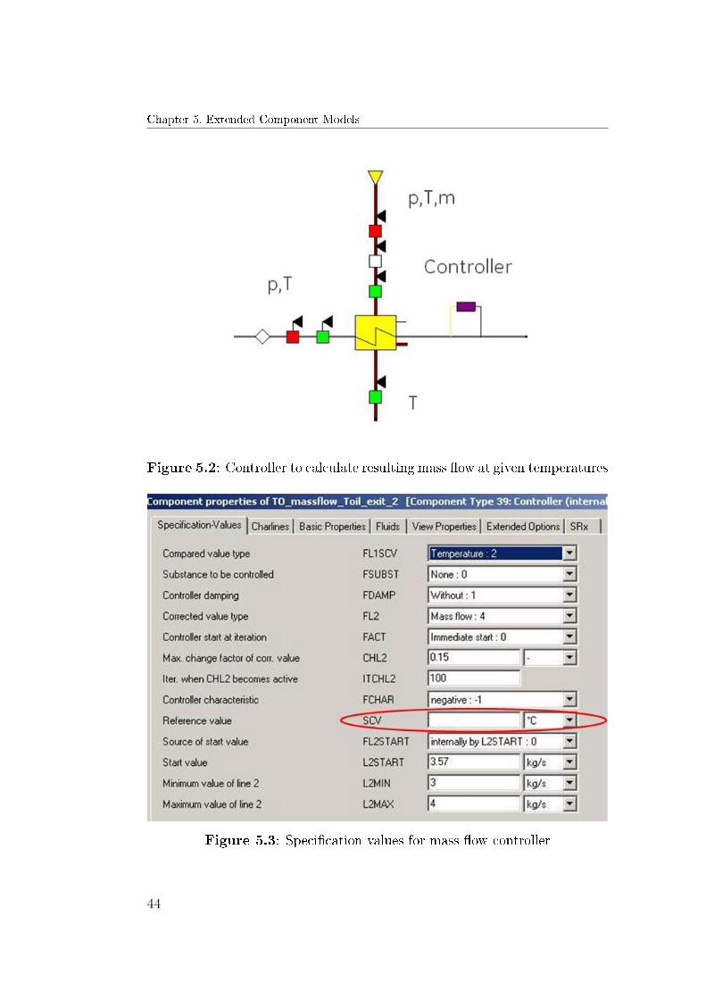
Chapter 5. Extended Component Models
Figure 5.2: Controller to calculate resulting mass �ow at given temperatures
Figure 5.3: Speci�cation values for mass �ow controller

Heat Exchanger Model
HX. Besides, three temperatures (green boxes), inlet pressure (red boxes)
and the mass �ow at the exhaust stream (white box) have been de�ned. A
legend with the EBSILON symbols displayed on the drawings can be found
at the Appendix (A.1).
5.1.3 O�-design Calculation
In this paragraph a closer look will be taken at the inputs for the o�-design
calculations. By performing a simulation under design conditions the heat
exchangers are dimensioned.
As mentioned in the previous section, the required heat transfer rate of the
CO.Ra cycle heat exchangers are calculated in the EBSILON design simula-
tion. This nominal value for UA can be calculated from the transferred heat
(see equation 5.3). By switching from design to o�-design mode this value is
stored as a reference value for the o�-design calculation. The same is valid
concerning the pressure drops. Both parameters are necessary to build an
o�-design model of the heat exchangers.
Concerning the UA, the heat transfer area naturally remains constant under
all boundary conditions, but this is not the case for the heat transfer coe�-
cient U. In the o�-design scenarios U in the heat exchangers will vary. Next,
the method to calculate the heat transfer rate (UA) in o�-design is explained.
Using individual thermal resistances, it can be formulated as follows:
1
UA=
1
(hA)c+Rw +
1
(hA)h(5.4)
where A is the heat transfer area. Subscripts c and h refer to the cold and
hot side of the heat exchanger, respectively. Neglecting the wall conduction
term Rw and assuming that the heat transfer coe�cient of the cold side (for
instance) is much larger compared to the hot side hc >> hh equation 5.4 can
be then simpli�ed to:1
UA=
1
(hA)h(5.5)
The area A is constant when comparing design to o�-design conditions. Using
Chapter 5. Extended Component Models
the Nusselt number and an empirical correlation including the Reynolds and
Prandtl numbers [22]:
Nu =hD
k= C ·RemD · Prn (5.6)
The constants C, m, and n, are assumed independent of the nature of the
�uid. Moreover, the Prandtl number Pr and thermal conductivity k are as-
sumed constant from design to o�-design conditions. In order to understand
the o�-design performance of the HX, it is of interest to state a relationship
between the o�-design UA and the design (UA)d. By using Re = m·DA·µ , where
the dynamic viscosity µ is assumed constant, a simple expression for the cor-
rection of the UA-value when going from design to o�-design simulations can
be derived:
UA
(UA)d=
RemDRemD,d
UA
(UA)d=
(m
md
)m (5.7)
The m-constant is dependent on the geometry of the heat exchanger. m is
the �uid mass �ow and subscript d refers to design conditions.
According to equation 5.7, the heat transfer coe�cient in the o�-design situa-
tion depends on the variation �ow on both sides of the HX. Heat exchangers
vendors usually furnish charts describing the UA variation depending on the
mass �ow on the primary or secondary side.
In EBSILON the UA value and the pressure drops of the o�-design calcula-
tions result from the UA value and the pressure losses of the design calcu-
lation multiplied by a correction factor (FK1 and FK2) that is determined
by characteristic lines. The user is able to implement such characteristic
lines for both sides of the heat exchanger. Using the characteristic lines the
following equation is used:
UA
(UA)d= FK1 · FK2 (5.8)

Heat Exchanger Model
These correction factors express the relationship between the �ows in both
calculation modes (FK1 for primary side and FK2 for secondary side). In the
o�-design mode then, an o�-design UA is then calculated from this nominal
UA by using the physical laws. An option, an adaptation polynomial (in
addition or as replacement) can also be de�ned for the o�-design scaling.
Regarding the pressure drops, by using m = ρ ·u ·A, and comparing to design
conditions the following expression can be derived for o�-design considera-
tions:
∆p = u2 ·K · ρ2
∆p
(∆p)d=
(ρdρ
)(m
md
)2 (5.9)
Knowing the nominal values in a design situation, the UA-value and the
pressure drops in an o�-design situation can be easily calculated with the
formulas stated in this section. As a result of the existing correlations in
EBSILON, in o�-design the UA and the pressure drops depending on �ow
conditions are known and the temperatures are calculated (see �gure 5.1).
5.1.4 Issues in modelling
Comparing the capabilities of the heat exchanger in EBSILON and in HYSYS
one issue was observed. The standard HX in EBSILON does not consider
phase change correctly as the heating curves at both HX sides are considered
linear; even if phase change occurs.
This heat exchanger model corresponds to the end point design model in
HYSYS, which considers only the temperatures at the entrance and the out-
let of the HX. This results in an incorrect logarithmic mean temperature dif-
ference value (LMTD) and consequently, in an incorrect heat transfer rate.
Figure 5.4 shows the T-Q diagram for a single cell where the phase change
of the working �uid occurs. The continuous lines correspond to the real be-
haviour of the �uid in the HX whereas the dotted line represents the curve
which is considered in EBSILON for the LMTD calculation.

Chapter 5. Extended Component Models
Figure 5.4: Phase transition at the standard heat exchanger model
In case the �uid experiments phase change, it becomes necessary to deter-
mine the LMTD for the preheating, the evaporating and the superheating
stage if included. For this purpose, a multiple-cell HX model has been de-
veloped to correctly account for phase change.
As seen in �gure 5.5 the HX has been split in stages or zones, setting di�erent
enthalpy steps (blue boxes) between them. By splitting in multiple cells, the
heating curves are broken into intervals and an energy balance is performed
along each interval. Consequently, a LMTD and a UA value for each cell
is calculated. These di�erent LMTD values are then combined to a single
value which represents the whole heat exchanger. Each interval at the T-Q
diagram depicted in �gure 5.6 corresponds to a cell of the HX.
This extended HX model has been built inside a macro. Modelling a cycle
using macros enables the user to create new components by grouping together
single components which can be integrated in the models as "black boxes".

Heat Exchanger Model
Figure 5.5: Multiple-cell heat exchanger model
Figure 5.6: Phase transition at the extended heat exchanger model
Additionally, this macro-mechanism allows to store and reuse sections of the
model for other cycle con�gurations. Moreover, as mentioned in section 3.1,
macros o�er the possibility to run a user de�ned program (EbsScript) before
Chapter 5. Extended Component Models
and after the calculation. For the CO.Ra cycle HXs, it has been implemented
for both cases; before and after the calculation.
The EbsScript, which is called automatically before the calculation, sets the
enthalpy steps and the pressure drops at each cell of the HX. Thus, if the
boundary conditions change or the number of cells increases, the user does
not need to set the steps manually.
The EbsScript to run after the calculation displays the calculated LMTD and
UA value for each cell. To derive a LMTD value for the entire heat exchanger
the values of the di�erent stages are combined. Each single LMTD is weighted
with the overall heat transfer coe�cient at the corresponding stage [23]. It
can be calculated as follows:
LMTDtot =1
ΣUAiΣLMTDi · UAi
LMTDtot =Qtot
UAtot
(5.10)
Besides the LMTD and UA value for the whole HX, the total thermal duty
and the minimum approach are also shown. The minimum approach is de-
�ned as the di�erence between the hot and cold pinch temperatures. In order
to calculate it in the multiple-cell model, the upper and lower terminal tem-
perature di�erence at each cell are compared. As a result, the lowest value
is then displayed. In other words, the accuracy of the minimum approach
depends on the number of cells. The higher the number of cells, the shorter
will be the intervals in the heating curves and therefore, the more precise will
be the phase change point considered.
The print-outputs of both EbsScripts for each HX can be viewed after the
calculation in the EbsKernel output bar which can be activated from the
menu command "View". An example of these scripts can be found at the
Appendix (A.3.1).
Pump Model
5.2 Pump Model
5.2.1 Technical Background
The selection of the pump type depends on the design volume �ow and the
design total head. Pumps are generally classi�ed as rotodynamic pumps and
positive displacement pumps.
The positive displacement pump operates by alternating the �lling of a cavity
with displacing a given volume of liquid. The �uid admitted in the working
chamber is isolated from the pump inlet and outlet. Then the �uid volume of
this chamber is decreased (e.g. with help of a piston), increasing the pressure
of the �uid which is �nally displaced to the pump outlet. The positive dis-
placement pump provides an approximate constant �ow at constant speed.
On the other hand, rotodynamic or centrifugal pumps produce a head and a
�ow by increasing the velocity of the liquid through the machine with the help
of a rotating vane impeller. The increase of kinetic energy is then converted
into static pressure [24]. This type of pump accounts for a large proportion
(upwards of 80%) of all pumps used on process plants [25].
Even if centrifugal pumps maximal head is lower than positive displacement
pumps maximal head, they have the advantage to be able to furnish higher
and constant volume �ow while positive displacement pumps are pulsate,
meaning that their volume �ow within a cycle is not constant [26]. As seen
in �gure 5.7 [26] the centrifugal pump can be categorised in di�erent groups:
radial, mixed and axial �ow pumps.
Because of the higher and constant volume �ows, centrifugal multi-stage
radial �ow pumps have been chosen for each of the three loops of the CO.Ra
cycle.
Pumps are designed not only for a speci�c combination of operating values
such as �ow rate, head or power consumption but for variable operational
data. The performance of a centrifugal pump is shown by a set of performance
curves. These characteristic lines show the dependency of the head, power
demand, the e�ciency and the NPSH on the �ow rate Q (�gure 5.8).

Chapter 5. Extended Component Models
Figure 5.7: Flow and head for di�erent types of centrifugal pumps
Figure 5.8: Typical performance curves for a centrifugal pump

Pump Model
Figure 5.9: Development of pressure through a centrifugal pump
In general, these pump maps are provided by the vendor and are used to
predict the o�-design behaviour of the pump.
Another technical aspect which has to be considered when designing a cen-
trifugal pump is cavitation. Cavitation is de�ned as the formation of vapour
bubbles of a �owing liquid in a region where the pressure of the liquid falls
below its vapour pressure (�gure 5.9 yellow dot). These bubbles collapse (im-
plode) when the pressure rises (�gure 5.9 red dot) and release shock waves.
Consequently, impellers can be damaged by the energy released [26]. In �g-
ure 5.9, (a) corresponds to the front of the impeller vanes and (b) to the
back.
Cavitation decreases �ow (Q) and head (H) which leads to reduced pump
performance. Furthermore, cavitation results in an increase of the noise
and vibrations, which can consequently damage bearings and shaft seals. In
order to avoid this, the net positive suction head (NPSH) is calculated. This
parameter will be explained in detail in section 5.2.3.
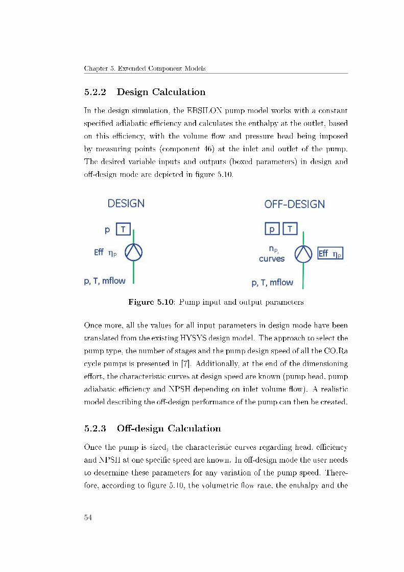
Chapter 5. Extended Component Models
5.2.2 Design Calculation
In the design simulation, the EBSILON pump model works with a constant
speci�ed adiabatic e�ciency and calculates the enthalpy at the outlet, based
on this e�ciency, with the volume �ow and pressure head being imposed
by measuring points (component 46) at the inlet and outlet of the pump.
The desired variable inputs and outputs (boxed parameters) in design and
o�-design mode are depicted in �gure 5.10.
Figure 5.10: Pump input and output parameters
Once more, all the values for all input parameters in design mode have been
translated from the existing HYSYS design model. The approach to select the
pump type, the number of stages and the pump design speed of all the CO.Ra
cycle pumps is presented in [7]. Additionally, at the end of the dimensioning
e�ort, the characteristic curves at design speed are known (pump head, pump
adiabatic e�ciency and NPSH depending on inlet volume �ow). A realistic
model describing the o�-design performance of the pump can then be created.
5.2.3 O�-design Calculation
Once the pump is sized, the characteristic curves regarding head, e�ciency
and NPSH at one speci�c speed are known. In o�-design mode the user needs
to determine these parameters for any variation of the pump speed. There-
fore, according to �gure 5.10, the volumetric �ow rate, the enthalpy and the

Pump Model
pressure at the inlet of the pump need to be set as an input. Moreover, the
a�nity laws have to be used to adapt the performance curves provided by
the supplier to every other speed.
First of all, the supplier characteristic curves need to be implemented. In
order to calculate the pressure increase it is necessary to derive a correla-
tion between the volume �ow and the delivered head of the pump. With a
suitable mathematical correlation representing the performance curve of the
pump and information about the current volumetric �ow rate, the delivered
head can be calculated. Together with the density of the �uid, the pressure
increase is determined. Equation 5.11 calculates the head delivered by the
low temperature feed pump at the CO.Ra cycle at a certain volumetric �ow
rate and at nominal speed. The �ow rate has to be set in (m3/h) and the
head is calculated in m.
H = −1 · 10−5 ·Q4 + 0.0007 ·Q3 − 0.0405 ·Q2 + 0.2692 ·Q+ 78.152 (5.11)
The pump e�ciency as a function of the inlet volumen �ow for the low
temperature pump is given by the following expression:
eta = 1 · 10−5 ·Q3 − 0.0015 ·Q2 + 0.0623 ·Q+ 0.0038 (5.12)
These regression equations have been obtained digitizing the characteristic
curves and plotting the data in EXCEL. The same has been done for the HT
and the thermal oil pump.
Since the pump speed will vary during the operation of CO.Ra equations
5.11 and 5.12 have to be adapted to the actual speed using the a�nity laws.
The a�nity laws allow an estimation of the head discharge and the e�ciency
characteristic at a di�erent speed or impeller diameter (than the measured
characteristic). With the impeller diameter (D) held constant, the following
equations apply with close approximation to how the change of speed of

Chapter 5. Extended Component Models
centrifugal pumps in�uences the performance of the pump:
Q1
Q2
=n1
n2
H1
H2
=n1
n2
2
P1
P2
=n1
n2
3
(5.13)
The a�nity laws apply on the condition that the system characteristic re-
mains unchanged for nn (nominal speed) and nx (reduced speed). Further-
more, the power equation implies that the pump e�ciency is unchanged for
the two speeds [26]. Figure 5.11 shows the e�ect of reduced speed (nx) on
the pump performance.
Once the performance curves and the a�nity laws are implemented, the
pump model calculates the pressure increase, the e�ciency, the required
power input and gives a warning if cavitation occurs. The net positive suction
head has to be calculated in order to detect cavitation. It can be expressed
in the following way:
NPSH =p0 − pvρ · g
(5.14)
The NPSH parameter shows the di�erence between the actual pressure of
a liquid in a pipeline (p0) and the liquid's vapour pressure (pv) at a given
temperature. NPSH can be either named NPSHr (required) or NPSHa
(available) where NPSHa is the available suction head in the system and
NPSHr the required suction head for the pump to avoid cavitation. The
latter is determined by reducing the suction head while the �ow is kept at
a constant level. When the di�erential pressure has decreased by 3 %, the
pressure at the pump's suction side is read; the NPSH value of the pump
is de�ned. This testing is repeated at di�erent �ow levels, which form the
basis of the NPSH curve in the end. In other words, when the NPSH curve
is reached, the level of cavitation is so high that the head of the pump has
decreased by 3 %. When performing o�-design simulations of the pump, both
NPSHa and NPSHr will be compared. NPSHa is calculated according to

Pump Model
Figure 5.11: System characteristics for di�erent a�nity equations
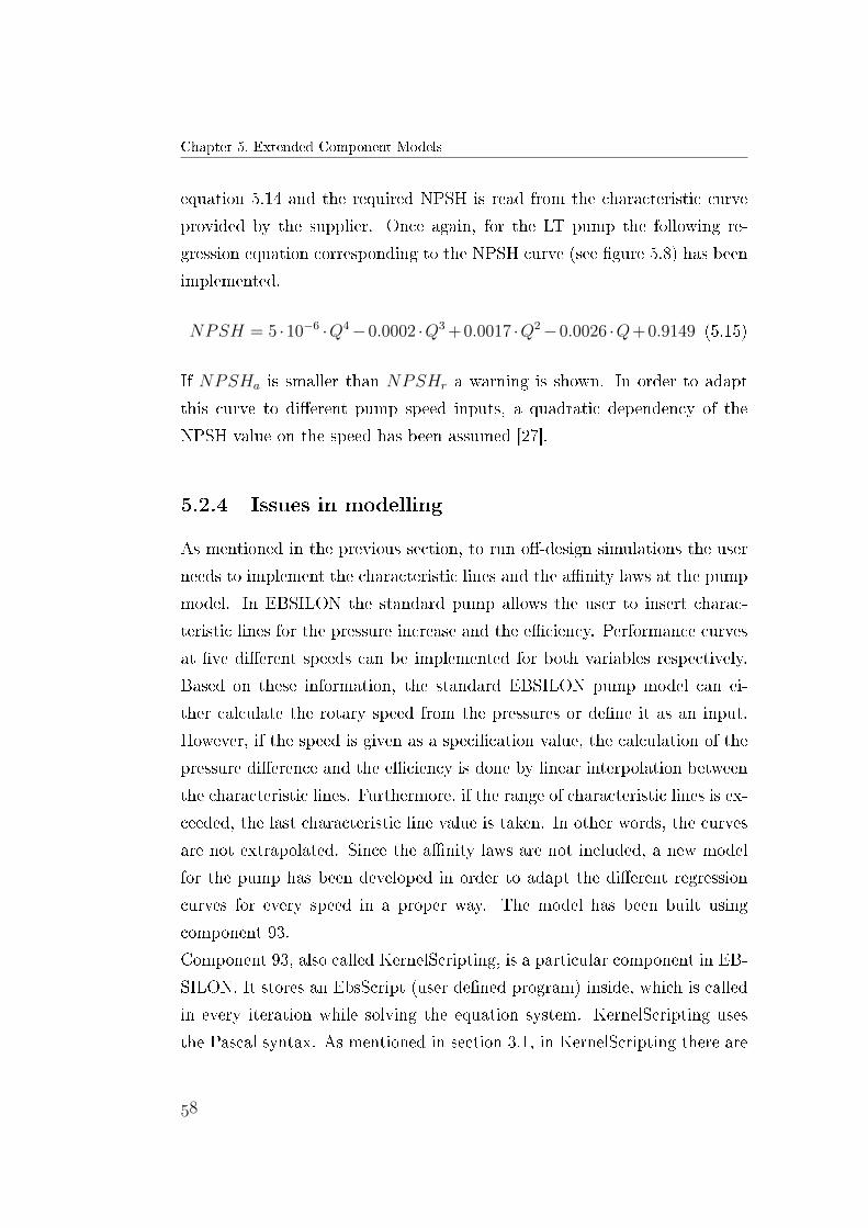
Chapter 5. Extended Component Models
equation 5.14 and the required NPSH is read from the characteristic curve
provided by the supplier. Once again, for the LT pump the following re-
gression equation corresponding to the NPSH curve (see �gure 5.8) has been
implemented.
NPSH = 5 ·10−6 ·Q4−0.0002 ·Q3 +0.0017 ·Q2−0.0026 ·Q+0.9149 (5.15)
If NPSHa is smaller than NPSHr a warning is shown. In order to adapt
this curve to di�erent pump speed inputs, a quadratic dependency of the
NPSH value on the speed has been assumed [27].
5.2.4 Issues in modelling
As mentioned in the previous section, to run o�-design simulations the user
needs to implement the characteristic lines and the a�nity laws at the pump
model. In EBSILON the standard pump allows the user to insert charac-
teristic lines for the pressure increase and the e�ciency. Performance curves
at �ve di�erent speeds can be implemented for both variables respectively.
Based on these information, the standard EBSILON pump model can ei-
ther calculate the rotary speed from the pressures or de�ne it as an input.
However, if the speed is given as a speci�cation value, the calculation of the
pressure di�erence and the e�ciency is done by linear interpolation between
the characteristic lines. Furthermore, if the range of characteristic lines is ex-
ceeded, the last characteristic line value is taken. In other words, the curves
are not extrapolated. Since the a�nity laws are not included, a new model
for the pump has been developed in order to adapt the di�erent regression
curves for every speed in a proper way. The model has been built using
component 93.
Component 93, also called KernelScripting, is a particular component in EB-
SILON. It stores an EbsScript (user de�ned program) inside, which is called
in every iteration while solving the equation system. KernelScripting uses
the Pascal syntax. As mentioned in section 3.1, in KernelScripting there are
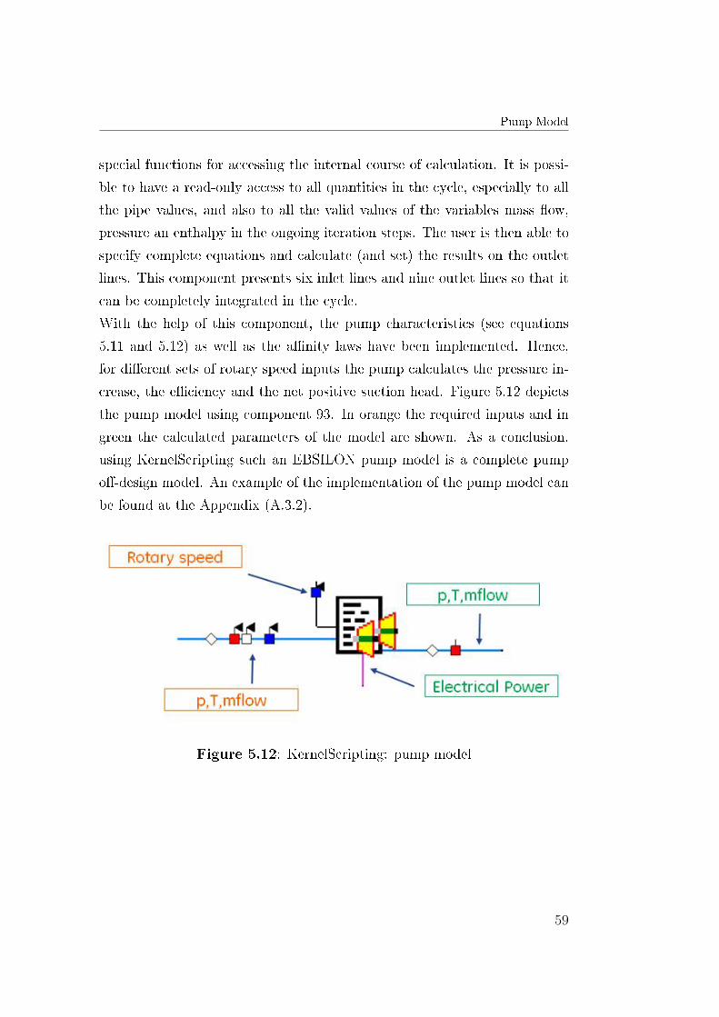
Pump Model
special functions for accessing the internal course of calculation. It is possi-
ble to have a read-only access to all quantities in the cycle, especially to all
the pipe values, and also to all the valid values of the variables mass �ow,
pressure an enthalpy in the ongoing iteration steps. The user is then able to
specify complete equations and calculate (and set) the results on the outlet
lines. This component presents six inlet lines and nine outlet lines so that it
can be completely integrated in the cycle.
With the help of this component, the pump characteristics (see equations
5.11 and 5.12) as well as the a�nity laws have been implemented. Hence,
for di�erent sets of rotary speed inputs the pump calculates the pressure in-
crease, the e�ciency and the net positive suction head. Figure 5.12 depicts
the pump model using component 93. In orange the required inputs and in
green the calculated parameters of the model are shown. As a conclusion,
using KernelScripting such an EBSILON pump model is a complete pump
o�-design model. An example of the implementation of the pump model can
be found at the Appendix (A.3.2).
Figure 5.12: KernelScripting: pump model
Chapter 5. Extended Component Models
5.3 Expander Model
5.3.1 Technical Background
CO.Ra was �rst designed to work with twin-screw machines as expansion
machines. Screw machines are classi�ed as positive displacement machines
and unlike turbomachines, in which the blading and stage requirements are
completely di�erent for expansion and compression, a screw compressor only
requires alteration to the high pressure port and reversal of direction of rota-
tion of the rotors to operate equally well as an expander. However, their e�-
ciencies as expanders are less well proven. The main feature of a twin-screw
expander design, which determines its adiabatic e�ciency, is the pro�le of the
rotors. These must form a good seal both between each other and between
the casing at all rotational positions in order to minimise internal leakage
[28]. Moreover, in most cases an internal oil lubrication system is necessary
in order to prevent seizure between the lobes. This results in a high cost of
seals to avoid gear and bearing lubrication oil mixing with the working �uid.
Further, the maximum adiabatic e�ciency of such an expander is relatively
low when comparing it to radial �ow turbines [28]. The lower adiabatic e�-
ciency led to a change in the CO.Ra design to radial �ow turbines.
In the radial turbine, �ow is changed from a radially inwards to axial di-
rection. In this case, the working �uid entering must be in the dry vapour
phase in order to maintain a high e�ciency and to prevent blade erosion by
any entrained mist of droplets. Moreover, the fact that turbine and genera-
tor are in one package results in a reduction of the maximum turbine inlet
temperature. However, this decrease is overcompensated by a turbine higher
e�ciency. The lack of need for an oil lubrication system and internal seals
as well as the use of magnetic bearings results in an increasing reliability.
To summarize, the signi�cant advantages o�ered by the radial turbine which
motivated to a design change are the higher e�ciency, the reliability and the
lower cost.
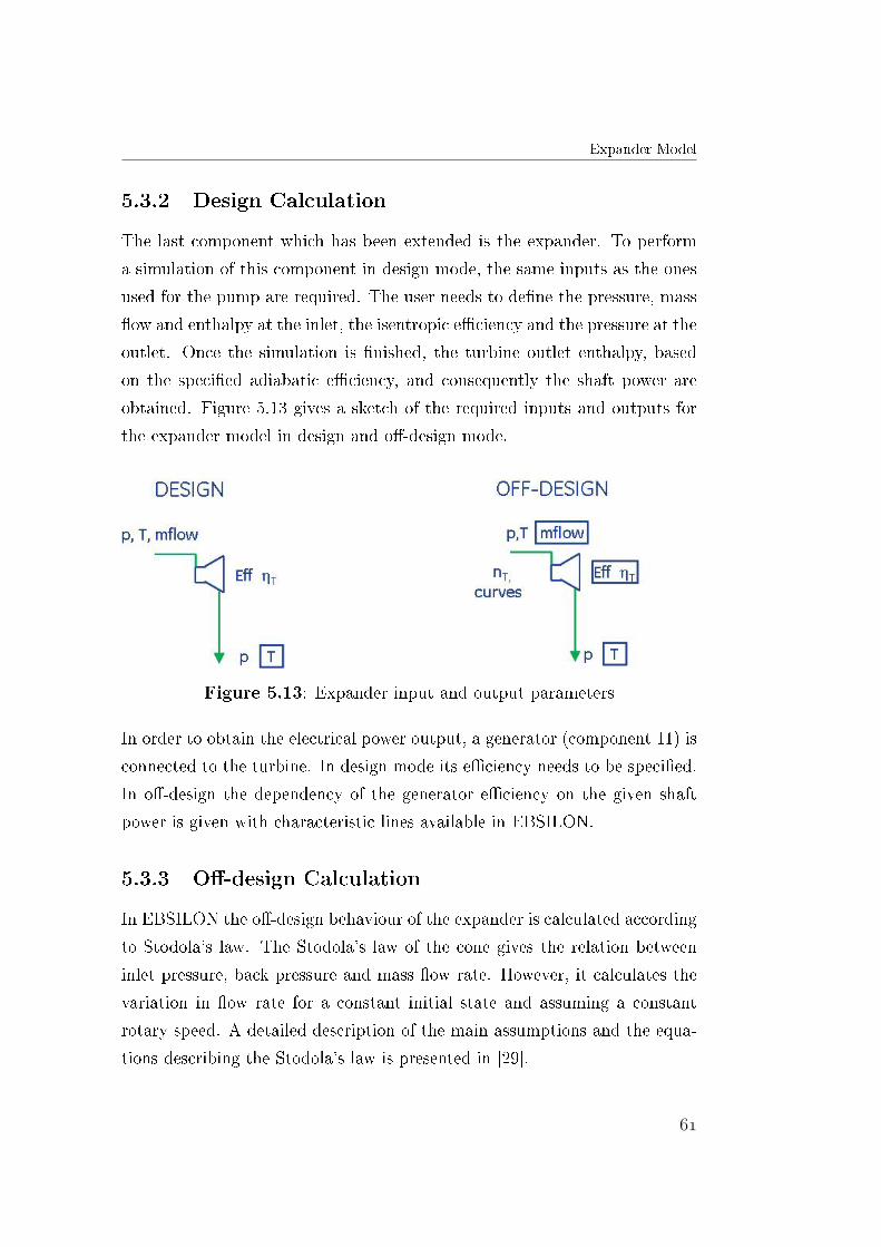
Expander Model
5.3.2 Design Calculation
The last component which has been extended is the expander. To perform
a simulation of this component in design mode, the same inputs as the ones
used for the pump are required. The user needs to de�ne the pressure, mass
�ow and enthalpy at the inlet, the isentropic e�ciency and the pressure at the
outlet. Once the simulation is �nished, the turbine outlet enthalpy, based
on the speci�ed adiabatic e�ciency, and consequently the shaft power are
obtained. Figure 5.13 gives a sketch of the required inputs and outputs for
the expander model in design and o�-design mode.
Figure 5.13: Expander input and output parameters
In order to obtain the electrical power output, a generator (component 11) is
connected to the turbine. In design mode its e�ciency needs to be speci�ed.
In o�-design the dependency of the generator e�ciency on the given shaft
power is given with characteristic lines available in EBSILON.
5.3.3 O�-design Calculation
In EBSILON the o�-design behaviour of the expander is calculated according
to Stodola's law. The Stodola's law of the cone gives the relation between
inlet pressure, back pressure and mass �ow rate. However, it calculates the
variation in �ow rate for a constant initial state and assuming a constant
rotary speed. A detailed description of the main assumptions and the equa-
tions describing the Stodola's law is presented in [29].
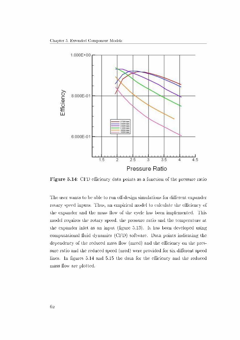
Chapter 5. Extended Component Models
Figure 5.14: CFD e�ciency data points as a function of the pressure ratio
The user wants to be able to run o�-design simulations for di�erent expander
rotary speed inputs. Thus, an empirical model to calculate the e�ciency of
the expander and the mass �ow of the cycle has been implemented. This
model requires the rotary speed, the pressure ratio and the temperature at
the expander inlet as an input (�gure 5.13). It has been developed using
computational �uid dynamics (CFD) software. Data points indicating the
dependency of the reduced mass �ow (mred) and the e�ciency on the pres-
sure ratio and the reduced speed (nred) were provided for six di�erent speed
lines. In �gures 5.14 and 5.15 the data for the e�ciency and the reduced
mass �ow are plotted.

Expander Model
Figure 5.15: CFD reduced mass �ow data points as a function of the pres-sure ratio
In EBSILON cubic regression equations have been implemented to build
the desired correlations. The model works as it follows. With the inputs
described above the reduced speed is calculated according to:
nred =n√
Tinlet(5.16)
where n stands for the expander rotary speed. Once the reduced speed is
calculated, the e�ciency and the reduced mass �ow can be obtained. As
mentioned previously, these values depend on the reduced speed and also the
pressure ratio. The reduced mass �ow is converted then to the mass �ow of
the cycle with equation 5.17.
m =mred · Pinlet√
Tinlet(5.17)

Chapter 5. Extended Component Models
Finally, with the result of the isentropic e�ciency, the expander outlet en-
thalpy is calculated. As data points for the regressions were only available in
a certain pressure ratio and reduced speed range the resulting reduced mass
�ows and e�ciencies are no longer credible when leaving this area. When
the cycle conditions are outside the speci�ed range a warning can be viewed
after the calculation in the Kernel output bar which can be activated from
the menu command "View".
5.3.4 Issues in modelling
KernelScripting has been used once more to specify the empirical regression
equations for the calculation of the expander e�ciency and the mass �ow.
However, instead of developing the whole model using this component, the
EBSILON standard steam turbine has been used.
First, the inlet temperature, pressure and back pressure, which are imposed
by other components in the loop, are imported to component 93. Therefore,
the KernelScripting component has to be connected to the inlet and outlet
pipe of the turbine by logical lines. By implementing special functions for
accessing the course of calculation, such as "ksGetPipeValue", the values for
the temperature and pressure at the inlet as well as the back pressure can be
read. Following, the e�ciency and mass �ow are calculated with the speci�ed
equations and set as a result at the KernelScripting output lines. To export
these values to the standard EBSILON turbine, one value transmitter for
the mass �ow and one for the outlet enthalpy have been used. These value
transmitters (component 36) help in modelling logical connections within a
model. In the case of the mass �ow, for example, the value transmitter ac-
cepts the value, which is calculated in KernelScripting and forwards it to the
inlet pipe of the turbine.
The model in EBSILON is constructed using on the one hand, KernelScript-
ing containing the empirical equations and on the other hand, taking advan-
tage of the standard EBSILON steam turbine to perform mass and energy
balances. Therefore, with the transmitted outlet enthalpy the adiabatic ef-

Expander Model
�ciency is calculated again at the turbine component. Moreover, once the
results are exported from component 93 to the turbine unit in the EBSILON
PFD, the electrical net output power can be �nally calculated. The connec-
tion between KernelScripting and the standard EBSILON turbine is shown
in �gure 5.16. The depicted parameters in green correspond to calculated
values and the orange ones to the required inputs.
Figure 5.16: KernelScripting: expander model
The EbsScript implemented for the low temperature turbine can be found at
the Appendix (A.3.3).

Chapter 6
Switch from Design to O�-Design
The main goal of CO.Ra is to produce additional electricity by using the heat
rejected from an engine without changing or disturbing its way of function-
ing. Therefore, it is particularly important that such systems can adapt to
changes in the gas engine operating point and in the ambient temperature.
To handle o�-design simulations, several pro�les with di�erent case studies
(di�erent sets of input data) will be created. As explained in chapter 3.1, the
use of this feature allows the user to manage variations of one cycle within
one document. By performing a calculation in design mode, the results cal-
culated by each component are stored and then used as reference values for
the o�-design calculation. Thus, the root of the pro�le hierarchy tree is al-
ways the design case. To change from design to o�-design the user simply
has to switch between the pro�les. In the CO.Ra model, when creating a
subpro�le (of the design root pro�le), the calculation is automatically per-
formed according to the o�-design rules. However, some adjustments have to
be made to the components of the basis model when switching to o�-design.
This chapter aims to give the steps to follow in order to set these component
and cycle modi�cations.
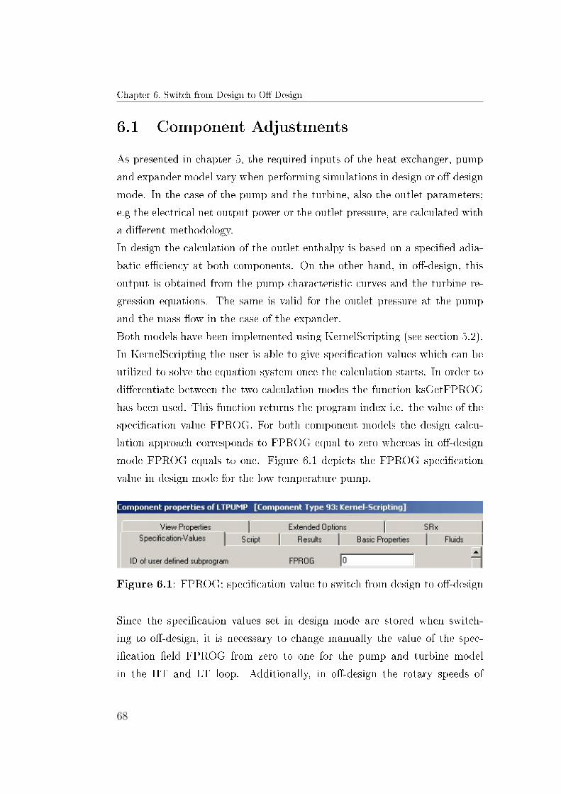
Chapter 6. Switch from Design to O�-Design
6.1 Component Adjustments
As presented in chapter 5, the required inputs of the heat exchanger, pump
and expander model vary when performing simulations in design or o�-design
mode. In the case of the pump and the turbine, also the outlet parameters;
e.g the electrical net output power or the outlet pressure, are calculated with
a di�erent methodology.
In design the calculation of the outlet enthalpy is based on a speci�ed adia-
batic e�ciency at both components. On the other hand, in o�-design, this
output is obtained from the pump characteristic curves and the turbine re-
gression equations. The same is valid for the outlet pressure at the pump
and the mass �ow in the case of the expander.
Both models have been implemented using KernelScripting (see section 5.2).
In KernelScripting the user is able to give speci�cation values which can be
utilized to solve the equation system once the calculation starts. In order to
di�erentiate between the two calculation modes the function ksGetFPROG
has been used. This function returns the program index i.e. the value of the
speci�cation value FPROG. For both component models the design calcu-
lation approach corresponds to FPROG equal to zero whereas in o�-design
mode FPROG equals to one. Figure 6.1 depicts the FPROG speci�cation
value in design mode for the low temperature pump.
Figure 6.1: FPROG: speci�cation value to switch from design to o�-design
Since the speci�cation values set in design mode are stored when switch-
ing to o�-design, it is necessary to change manually the value of the spec-
i�cation �eld FPROG from zero to one for the pump and turbine model
in the HT and LT loop. Additionally, in o�-design the rotary speeds of
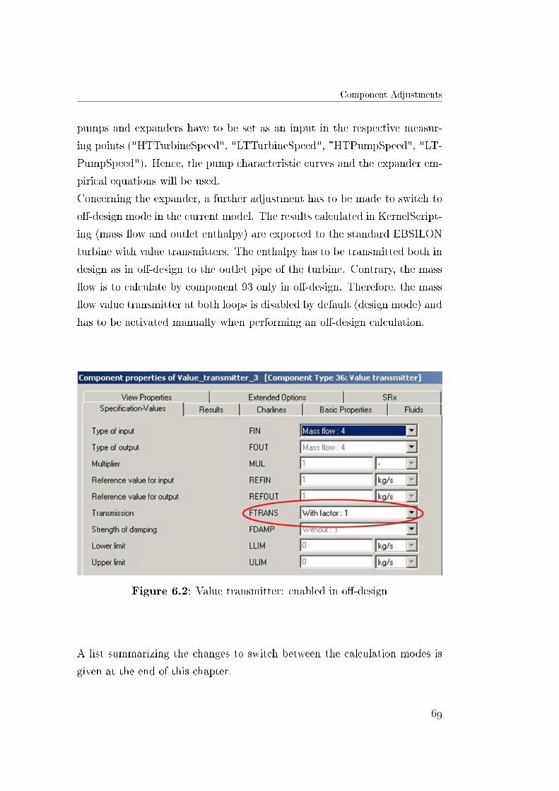
Component Adjustments
pumps and expanders have to be set as an input in the respective measur-
ing points ("HTTurbineSpeed", "LTTurbineSpeed", "HTPumpSpeed", "LT-
PumpSpeed"). Hence, the pump characteristic curves and the expander em-
pirical equations will be used.
Concerning the expander, a further adjustment has to be made to switch to
o�-design mode in the current model. The results calculated in KernelScript-
ing (mass �ow and outlet enthalpy) are exported to the standard EBSILON
turbine with value transmitters. The enthalpy has to be transmitted both in
design as in o�-design to the outlet pipe of the turbine. Contrary, the mass
�ow is to calculate by component 93 only in o�-design. Therefore, the mass
�ow value transmitter at both loops is disabled by default (design mode) and
has to be activated manually when performing an o�-design calculation.
Figure 6.2: Value transmitter: enabled in o�-design
A list summarizing the changes to switch between the calculation modes is
given at the end of this chapter.

Chapter 6. Switch from Design to O�-Design
6.2 Cycle Adjustments
To perform o�-design simulations some improvements were made to the dif-
ferent loops to make them successfully converge. Both the HT and LT loop
have been closed adopting several measures.
First, a mass �ow separator has been implemented at both loops to avoid an
over-determination in mass �ow. This splitter has to be set in every closed
circuit where no purge or feed stream is available. In EBSILON the once-
de�ned mass �ow is transmitted from component to component and at some
point encounters the position where it has been de�ned. This leads to an
over-determination warning. The mass �ow separator in each loop needs to
be enabled in both calculation modes. Moreover, depending on the loop,
further basic quantities (e.g. enthalpy) have to be split when switching the
calculation mode.
In o�-design the basis pressure of the loop is calculated by the condenser
and transferred to the pump inlet. When trying to close the LT loop, it
was observed that the pump was extremely sensitive to the pressure at the
pump inlet. Therefore, a pressure separator ("LTSeparator") has been set
at this position of the cycle. A controller ("LTPressureController") is then
used to transmit the pressure at the output of the condenser to the pump
inlet. Figure 6.3 depicts the splitter and controller at the LT loop. Inserting
a pressure splitter equals to start the simulation with an open cycle regard-
ing this quantity. Besides, controllers in EBSILON o�er the possibility to
give a start value for the calculation. The controller used for this purpose
di�ers from the one explained in section 5.1 in the fact that the scheduled
value is not a �xed number, but instead determined during the calculation.
In the case of the LT loop, the scheduled value corresponds to the saturation
pressure at the condenser. Figure 6.4 shows the required speci�cations for
this component. Notice that both the compared and the correction value are
the pressure.
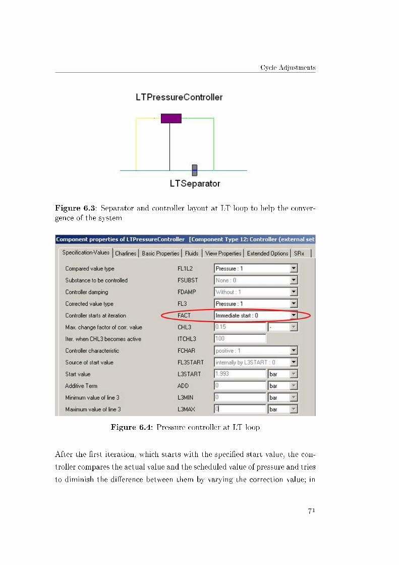
Cycle Adjustments
Figure 6.3: Separator and controller layout at LT loop to help the conver-gence of the system
Figure 6.4: Pressure controller at LT loop
After the �rst iteration, which starts with the speci�ed start value, the con-
troller compares the actual value and the scheduled value of pressure and tries
to diminish the di�erence between them by varying the correction value; in
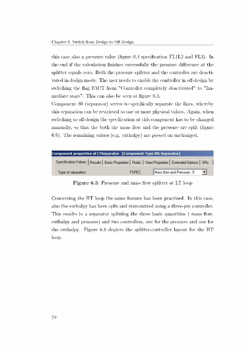
Chapter 6. Switch from Design to O�-Design
this case also a pressure value (�gure 6.4 speci�cation FL1L2 and FL3). In
the end if the calculation �nishes successfully the pressure di�erence at the
splitter equals zero. Both the pressure splitter and the controller are deacti-
vated in design mode. The user needs to enable the controller in o�-design by
switching the �ag FACT from "Controller completely deactivated" to "Im-
mediate start". This can also be seen at �gure 6.4.
Component 80 (separator) serves to speci�cally separate the lines, whereby
this separation can be restricted to one or more physical values. Again, when
switching to o�-design the speci�cation at this component has to be changed
manually, so that the both the mass �ow and the pressure are split (�gure
6.5). The remaining values (e.g. enthalpy) are passed on unchanged.
Figure 6.5: Pressure and mass �ow splitter at LT loop
Concerning the HT loop the same feature has been practised. In this case,
also the enthalpy has been split and transmitted using a three-pin controller.
This results in a separator splitting the three basic quantities ( mass �ow,
enthalpy and pressure) and two controllers, one for the pressure and one for
the enthalpy. Figure 6.6 depicts the splitter-controller layout for the HT
loop.
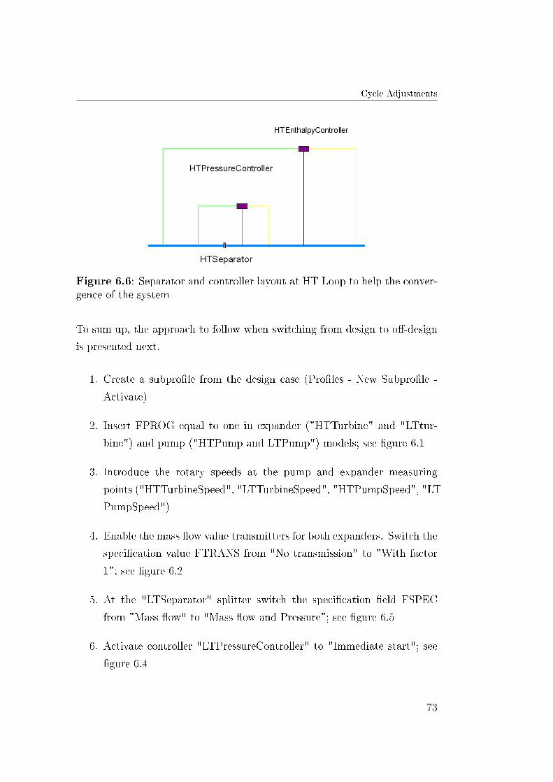
Cycle Adjustments
Figure 6.6: Separator and controller layout at HT Loop to help the conver-gence of the system
To sum up, the approach to follow when switching from design to o�-design
is presented next.
1. Create a subpro�le from the design case (Pro�les - New Subpro�le -
Activate)
2. Insert FPROG equal to one in expander ("HTTurbine" and "LTtur-
bine") and pump ("HTPump and LTPump") models; see �gure 6.1
3. Introduce the rotary speeds at the pump and expander measuring
points ("HTTurbineSpeed", "LTTurbineSpeed", "HTPumpSpeed", "LT-
PumpSpeed")
4. Enable the mass �ow value transmitters for both expanders. Switch the
speci�cation value FTRANS from "No transmission" to "With factor
1"; see �gure 6.2
5. At the "LTSeparator" splitter switch the speci�cation �eld FSPEC
from "Mass �ow" to "Mass �ow and Pressure"; see �gure 6.5
6. Activate controller "LTPressureController" to "Immediate start"; see
�gure 6.4

Chapter 6. Switch from Design to O�-Design
7. At the "HTSeparator" splitter switch the speci�cation �eld FSPEC
from "Mass �ow" to "Mass �ow, Pressure and Enthalpy"
8. Activate controller "HTPressureController" to "Immediate start"
9. Activate controller "HTEnthalpyController" to "Immediate start"
If the user wants to perform o�-design simulations for di�erent ambient tem-
peratures, the air supply temperature has to be changed at the boundary
input value called "Outside".
Once the adjustments described above have been set, the calculation will be
done according to the o�-design rules.

Chapter 7
O�-design Simulations
The CO.Ra power plant is designed and constructed to provide a rated power
output at full load of the gas engine and at speci�c ambient conditions. Due
to both diurnal and seasonal changes in the ambient air temperature, as
well as variations of the engine load, CO.Ra will seldom operate at design
conditions. A major quality aspect required in such ORC power plant is
the reproducibility of its system behaviour. Therefore, o�-design simulations
need to be calculated. This chapter aims to describe the model performance
in o�-design calculation mode. Further, a sensitivity analysis regarding both
pump rotary speeds (HT loop and LT loop) will be presented.
7.1 O�-design model
The integrated model of the cycle is built by interconnecting the models of
the HT and LT loops described in chapter 4. The thermal oil loop has not
been assembled in o�-design in order to simplify the simulations and reduce
the computational cost. Instead, as in the case of the engine cooling water
system, it has been reduced in the model to the Evaporator inlet and outlet
stream, with the inlet conditions corresponding to the design point.
The modelling highlights the following constraints:
• For a given rotary speed and mass �ow rate the pump imposes the
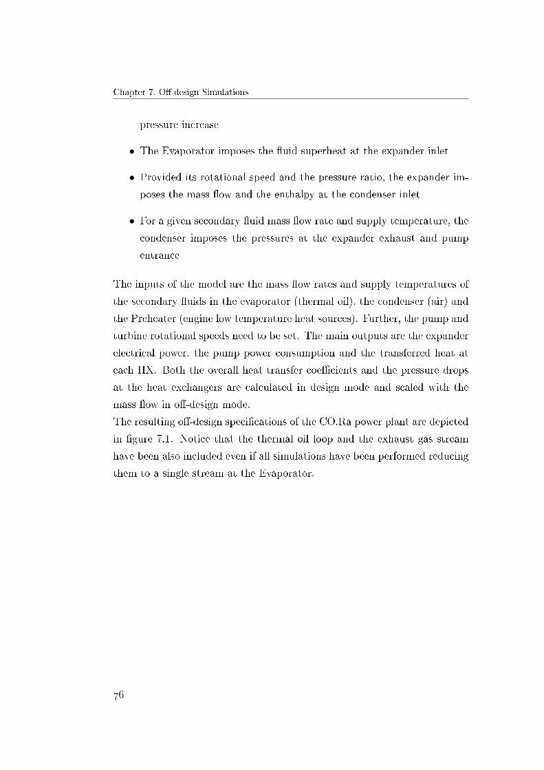
Chapter 7. O�-design Simulations
pressure increase
• The Evaporator imposes the �uid superheat at the expander inlet
• Provided its rotational speed and the pressure ratio, the expander im-
poses the mass �ow and the enthalpy at the condenser inlet
• For a given secondary �uid mass �ow rate and supply temperature, the
condenser imposes the pressures at the expander exhaust and pump
entrance
The inputs of the model are the mass �ow rates and supply temperatures of
the secondary �uids in the evaporator (thermal oil), the condenser (air) and
the Preheater (engine low temperature heat sources). Further, the pump and
turbine rotational speeds need to be set. The main outputs are the expander
electrical power, the pump power consumption and the transferred heat at
each HX. Both the overall heat transfer coe�cients and the pressure drops
at the heat exchangers are calculated in design mode and scaled with the
mass �ow in o�-design mode.
The resulting o�-design speci�cations of the CO.Ra power plant are depicted
in �gure 7.1. Notice that the thermal oil loop and the exhaust gas stream
have been also included even if all simulations have been performed reducing
them to a single stream at the Evaporator.

O�-design model
Figure 7.1: O�-design speci�cations

Chapter 7. O�-design Simulations
7.2 Sensitivity Analysis
As mentioned in section 2.2, the o�-design simulations carried out in this
work focus on the sensitivity analysis of the model and the calculation of the
rotary speeds of pumps to run the plant close to the design point. For the
analysis the expander speeds are set with a constant value and the pump
speeds are modi�ed. The inlet conditions of the secondary �uids exchanging
heat with the system (air, engine cooling water and thermal oil) also remain
constant. The HT and LT turbine are operated with 26200 and 21800 rpm
respectively. These speed values correspond to their optimal point of perfor-
mance (higher e�ciency). The design con�guration of 15◦C and 100 % load
is used as starting point for all o�-design simulations which are performed
steady-state.
First, several simulations with di�erent pump speed combinations were cal-
culated. To determine whether the model was providing consistent results,
the rotary speeds were modi�ed until the thermodynamic conditions at the
nominal point were reached. Moreover, by increasing/decreasing the HT/LT
pump speed, the behaviour of the model was analysed. All simulations were
calculated using the EXCEL Interface available in EBSILON.
In order to start the simulations with reasonable speed values, both loops
were simulated separately to calculate their "nominal" pump rotary speed;
i.e, speed at which the thermodynamic conditions equal the design conditions.
As mentioned in chapter 5.3, both loops use radial turbines as expansion ma-
chines. Therefore, a certain degree of superheat has to be ensured to avoid
droplets at the turbine blades. The design point operates with 10 K and 20
K superheat at the HT and LT loop respectively. On the other hand, the
expander inlet temperature cannot exceed speci�c maximum values, since
it would result in a lack of cooling for the integrated generator. Thus, the
turbine inlet conditions (temperature and superheat) have been chosen as
boundary requirements when selecting the pump nominal speeds. Tables 7.1
and 7.2 show the obtained nominal speeds (for the separated loops) as well as
the deviation of the resulting conditions to the design point. The deviations
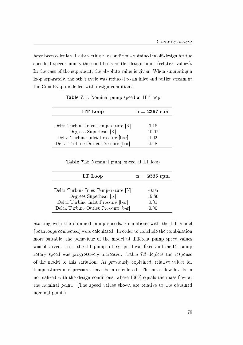
Sensitivity Analysis
have been calculated subtracting the conditions obtained in o�-design for the
speci�ed speeds minus the conditions at the design point (relative values).
In the case of the superheat, the absolute value is given. When simulating a
loop separately, the other cycle was reduced to an inlet and outlet stream at
the CondEvap modelled with design conditions.
Table 7.1: Nominal pump speed at HT loop
HT Loop n = 2397 rpm
Delta Turbine Inlet Temperature [K] 0.16Degrees Superheat [K] 10.02
Delta Turbine Inlet Pressure [bar] 0.02Delta Turbine Outlet Pressure [bar] 0.48
Table 7.2: Nominal pump speed at LT loop
LT Loop n = 2336 rpm
Delta Turbine Inlet Temperature [K] -0.06Degrees Superheat [K] 19.80
Delta Turbine Inlet Pressure [bar] 0.01Delta Turbine Outlet Pressure [bar] 0.00
Starting with the obtained pump speeds, simulations with the full model
(both loops connected) were calculated. In order to conclude the combination
more suitable, the behaviour of the model at di�erent pump speed values
was observed. First, the HT pump rotary speed was �xed and the LT pump
rotary speed was progressively increased. Table 7.3 depicts the response
of the model to this variation. As previously explained, relative values for
temperatures and pressures have been calculated. The mass �ow has been
normalized with the design conditions, where 100% equals the mass �ow at
the nominal point. (The speed values shown are relative to the obtained
nominal point.)
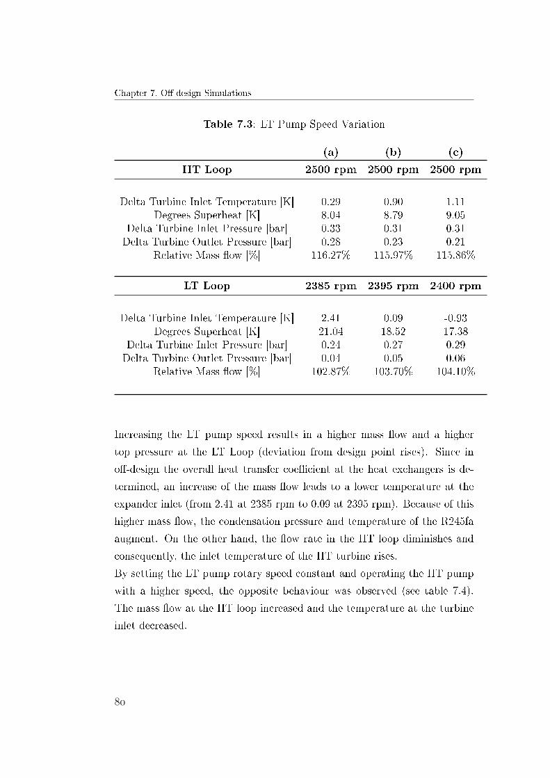
Chapter 7. O�-design Simulations
Table 7.3: LT Pump Speed Variation
(a) (b) (c)
HT Loop 2500 rpm 2500 rpm 2500 rpm
Delta Turbine Inlet Temperature [K] 0.29 0.90 1.11Degrees Superheat [K] 8.04 8.79 9.05
Delta Turbine Inlet Pressure [bar] 0.33 0.31 0.31Delta Turbine Outlet Pressure [bar] 0.28 0.23 0.21
Relative Mass �ow [%] 116.27% 115.97% 115.86%
LT Loop 2385 rpm 2395 rpm 2400 rpm
Delta Turbine Inlet Temperature [K] 2.41 0.09 -0.93Degrees Superheat [K] 21.04 18.52 17.38
Delta Turbine Inlet Pressure [bar] 0.24 0.27 0.29Delta Turbine Outlet Pressure [bar] 0.04 0.05 0.06
Relative Mass �ow [%] 102.87% 103.70% 104.10%
Increasing the LT pump speed results in a higher mass �ow and a higher
top pressure at the LT Loop (deviation from design point rises). Since in
o�-design the overall heat transfer coe�cient at the heat exchangers is de-
termined, an increase of the mass �ow leads to a lower temperature at the
expander inlet (from 2.41 at 2385 rpm to 0.09 at 2395 rpm). Because of this
higher mass �ow, the condensation pressure and temperature of the R245fa
augment. On the other hand, the �ow rate in the HT loop diminishes and
consequently, the inlet temperature of the HT turbine rises.
By setting the LT pump rotary speed constant and operating the HT pump
with a higher speed, the opposite behaviour was observed (see table 7.4).
The mass �ow at the HT loop increased and the temperature at the turbine
inlet decreased.
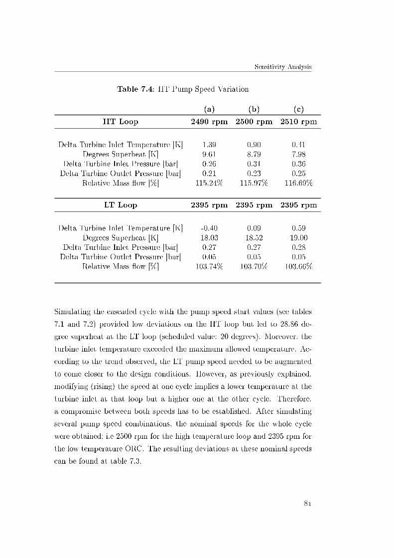
Sensitivity Analysis
Table 7.4: HT Pump Speed Variation
(a) (b) (c)
HT Loop 2490 rpm 2500 rpm 2510 rpm
Delta Turbine Inlet Temperature [K] 1.39 0.90 0.41Degrees Superheat [K] 9.61 8.79 7.98
Delta Turbine Inlet Pressure [bar] 0.26 0.31 0.36Delta Turbine Outlet Pressure [bar] 0.21 0.23 0.25
Relative Mass �ow [%] 115.24% 115.97% 116.69%
LT Loop 2395 rpm 2395 rpm 2395 rpm
Delta Turbine Inlet Temperature [K] -0.40 0.09 0.59Degrees Superheat [K] 18.03 18.52 19.00
Delta Turbine Inlet Pressure [bar] 0.27 0.27 0.28Delta Turbine Outlet Pressure [bar] 0.05 0.05 0.05
Relative Mass �ow [%] 103.74% 103.70% 103.66%
Simulating the cascaded cycle with the pump speed start values (see tables
7.1 and 7.2) provided low deviations on the HT loop but led to 28.86 de-
gree superheat at the LT loop (scheduled value: 20 degrees). Moreover, the
turbine inlet temperature exceeded the maximum allowed temperature. Ac-
cording to the trend observed, the LT pump speed needed to be augmented
to come closer to the design conditions. However, as previously explained,
modifying (rising) the speed at one cycle implies a lower temperature at the
turbine inlet at that loop but a higher one at the other cycle. Therefore,
a compromise between both speeds has to be established. After simulating
several pump speed combinations, the nominal speeds for the whole cycle
were obtained; i.e 2500 rpm for the high temperature loop and 2395 rpm for
the low temperature ORC. The resulting deviations at these nominal speeds
can be found at table 7.3.
Chapter 7. O�-design Simulations
Once the pump nominal speeds were known, the e�ciency of the cycle was
calculated. The e�ciency of the cascaded cycle is de�ned according to equa-
tion 7.1.
ηORC =Pturbines − Ppumps
QEvaporator +QPreheater
(7.1)
Once more, the pump speeds were varied around the nominal values to on
the one hand, simulate and evaluate their impact on the cycle e�ciency
and on the other hand, to check up on whether the chosen nominal point
corresponded to the optimal point. It should be mentioned that since the air-
cooled condenser model does not include the electric consumption of the fans,
the power consumption of these has not been considered for the e�ciency
calculation. Following the same procedure, the HT pump speed was modi�ed
setting the LT pump to a constant value of 2395 rpm (nominal speed). For
each pump speed combination the e�ciency was calculated and normalized
with the design conditions (100 % equals the design e�ciency). Figure 7.2
shows the results of this �rst series of simulations.
After, the same procedure was followed varying the LT pump speed and
�xing the HT pump speed to 2500 rpm (see �gure 7.3).
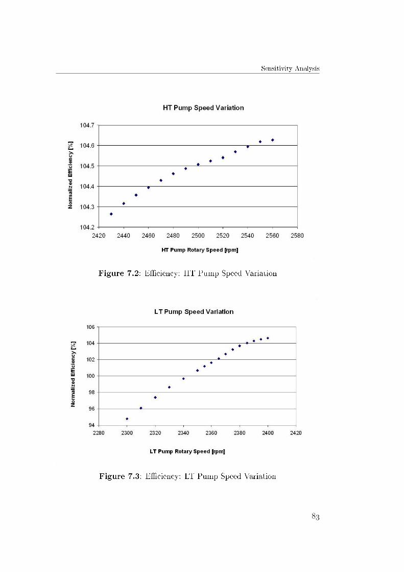
Sensitivity Analysis
Figure 7.2: E�ciency: HT Pump Speed Variation
Figure 7.3: E�ciency: LT Pump Speed Variation
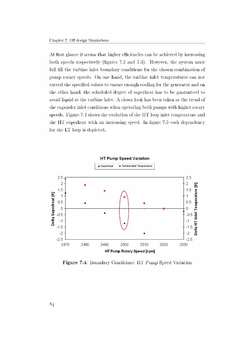
Chapter 7. O�-design Simulations
At �rst glance it seems that higher e�ciencies can be achieved by increasing
both speeds respectively (�gures 7.2 and 7.3). However, the system must
full �ll the turbine inlet boundary conditions for the chosen combination of
pump rotary speeds. On one hand, the turbine inlet temperatures can not
exceed the speci�ed values to ensure enough cooling for the generator and on
the other hand, the scheduled degree of superheat has to be guaranteed to
avoid liquid at the turbine inlet. A closer look has been taken at the trend of
the expander inlet conditions when operating both pumps with higher rotary
speeds. Figure 7.4 shows the evolution of the HT loop inlet temperature and
the HT superheat with an increasing speed. In �gure 7.5 such dependency
for the LT loop is depicted.
Figure 7.4: Boundary Conditions: HT Pump Speed Variation
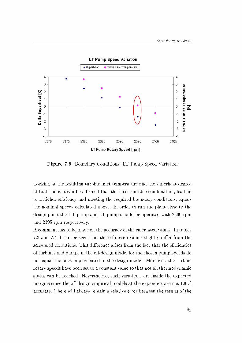
Sensitivity Analysis
Figure 7.5: Boundary Conditions: LT Pump Speed Variation
Looking at the resulting turbine inlet temperature and the superheat degree
at both loops it can be a�rmed that the most suitable combination, leading
to a higher e�ciency and meeting the required boundary conditions, equals
the nominal speeds calculated above. In order to run the plant close to the
design point the HT pump and LT pump should be operated with 2500 rpm
and 2395 rpm respectively.
A comment has to be made on the accuracy of the calculated values. In tables
7.3 and 7.4 it can be seen that the o�-design values slightly di�er from the
scheduled conditions. This di�erence arises from the fact that the e�ciencies
of turbines and pumps in the o�-design model for the chosen pump speeds do
not equal the ones implemented in the design model. Moreover, the turbine
rotary speeds have been set to a constant value so that not all thermodynamic
states can be reached. Nevertheless, such variations are inside the expected
margins since the o�-design empirical models at the expanders are not 100%
accurate. There will always remain a relative error between the results of the

Chapter 7. O�-design Simulations
design model and the o�-design model when varying only the pump speeds.
Chapter 8
Outlook and Conclusion
Within the scope of this thesis, a model of a cascaded Organic Rankine Cy-
cle plant (CO.Ra) for waste heat recovery has been established. EBSILON
has been the platform for the development of the model. Its dedicated o�-
design calculation mode and the existence of a user de�ned script (EbsScript)
encouraged to use EBSILON in order to perform steady-state ORC simula-
tions. The main goal of this thesis was to determine whether EBSILON was
suitable or not for this purpose.
In order to match the simulation requirements the following components have
been extended:
• A multiple-cell heat exchanger model has been developed to correctly
account for phase change. By setting enthalpy steps between the cells,
the heating curves are divided into several stages and an energy balance
is performed in each interval. This model has been built using a macro,
where EbsScripts, which are called automatically before and after the
calculation have been implemented.
• A pump model has been created implementing the characteristic lines
for head, e�ciency, NPSH and the a�nity laws to consider the e�ects
at speed change. The model has been developed using KernelScripting.
• Regarding the expander, KernelScripting has been used to specify re-

Chapter 8. Outlook and Conclusion
gression equations for the calculation of the expander e�ciency and
the mass �ow. This empirical model has been developed using CFD
calculation. Moreover, it has been taken advantage of the standard
EBSILON turbine to perform mass and energy balances.
Individual component performance has been modelled to vary with changes
in �ow rates so that the modelled plant's response to variations in boundary
and ambient conditions would be indicative of an actual plant's response.
Further, an integrated model of the whole installation has been assembled in
design and o�-design mode. The plant and components were sized to produce
the desired power output for speci�ed resource and ambient conditions (15
degrees ambient temperature and the engine at full load). This �xed con�g-
uration plant has then been used to evaluate performance under o�-design
resource scenarios.
In order to analyse the behaviour of the model outside of the design point, a
�rst parametric study has been carried out simulating the model at o�-design
conditions. Hence, the most suitable combination for the HT and LT pump
rotary speed in order to run the cascaded organic cycle close to the design
point has been calculated. This sensitivity analysis concluded that the re-
sults provided by the model are in agreement with the expected behaviour.
Looking at the current status of the model and having succeeded in modelling
the component performance in order to match the simulation requirements,
it is stated that the main goal of the thesis has been achieved. The simulation
software EBSILON together with the new user added functions is proved to
be an accurate tool to run ORC simulations both under design and o�-design
conditions.

For a further development of the model, the bypasses and valves to control
the heat input at the ORC need to be included. The R245fa loop is controlled
with a Preheater bypass to regulate the heat input and variable pump speed.
The high temperature loops are controlled using a bypass on the TO side of
the Evaporator along with cyclohexane and thermo-oil pumps with variable
speed. Additionally, a valve to bypass the exhaust heat exchanger has to be
modelled.
A more advanced step would be to build a pressure drop and heat loss model
to simulate the pressure losses caused by the piping system.
Another step could be the integration of variable speed condenser fans. Since
the condenser speed is also used as control variable, this could improve the
accuracy of the model.
A comment should be made to the currently used EBSILON version. As
previously mentioned, a multiple-cell heat exchanger model has been devel-
oped to consider non linear heating curves. This component design as well
as further interesting �uids for ORC applications will be included in the next
version of the program.
To conclude, in order to obtain accurate results, the �nal step would be the
calibration and validation of the model. To validate the o�-design behaviour
simulated in this work, measurement data from an existing prototype should
be used.

Bibliography
[1] E. C. Energy, �European energy and transport - trends to 2030,� tech.
rep., 2007.
[2] I. E. Agency, �World energy outlook 2010,� tech. rep.,
www.worldenergyoutlook.com -accessed on 03.08.2010.
[3] P.G.Stecher, Industrial and Institutional Waste Heat Recovery. Noyes
Data Corporation, 1979.
[4] R. Davies and J. Holbery, Opportunity Analysis for Recovering Energy
from Industrial Waste Heat and Emissions. Paci�c Northwest National
Laboratory, 2006.
[5] M. Sakhavi, �Waste heat recovery using rankine cycles,� in VDI Berichte
539, Verein Deutscher Ingenieure.
[6] Bureau of Energy E�ciency, http://www.em-ea.org/Guide
Books/book-2/2.8 Waste Heat Recovery.pdf, Energy E�ciency in
Thermal Utilities. - accessed on 25.08.10.
[7] P. Huck, �System analysis for organic rankine cycle applications,� Mas-
ter's thesis, TU München, 2007.
[8] M. F. Hordeski, Dictionary of Energy E�ciency Technologies. 2004.
[9] Turboboden. http://www.turboden.eu/en/rankine/rankine-
history.php. -accessed on 15.09.10.
BIBLIOGRAPHY
[10] J.Larjola, �Electricity from industrial waste heat using high speed or-
ganic rankine cycle (orc),� tech. rep., Department of Energy Technology,
Lappeenranta University of Technology, 1995.
[11] A.Schuster and S. Karellas, �Energetic and economic investigation of or-
ganic rankine cycle applications,� tech. rep., Institute for Energy Sytems,
Technische Universität München, 2008.
[12] J.Karl, Dezentrale Energiesysteme. Neue Technologien im liberalisierten
Energiemarkt. München, Oldenbourg, 2006.
[13] R. Vescovo, �Organic rankine cycle recovering industrial heat,� tech.
rep., Turboden, 2009.
[14] H. Gurgenci, �Performance of power plants with organic rankine cycles
under part-load and o�design conditions,� tech. rep., Solar Energy Re-
search Centre, University of Queensland, 1985.
[15] S. Consonni, �O�-design performance of integrated waste-to-energy,
combined cycle plants,� tech. rep., Department of Energy Engineering,
Politecnico di Milano, 2007.
[16] P. J. Mago, �An examination of regenerative organic rankine cycles using
dry �uids,� tech. rep., Department of Mechanical Engineering, Missis-
sippi State University, 2007.
[17] U. Drescher and D. Brüggemann, �Fluid selection for the organic
rankine cycle (orc) in biomass power and heat plants,� tech. rep.,
Lehrstuhl für Technische Thermodynamic und Transportprozesse, Uni-
versität Bayreuth, 2006.
[18] T. Emperho�, �Design of an organic rankine cycle in combination with a
ge jenbacher engine,� Master's thesis, Fachhochschule Regensburg, 2007.

BIBLIOGRAPHY
[19] A. Borsukiewicz-Gozdur, �Comparative analysis of natural and synthetic
refrigerants in application to low temperature clausius rankine cycle,�
tech. rep., Szczecin University of Technology, 2005.
[20] �http://www51.honeywell.com.� - accessed on 15.10.2010.
[21] B.-T. Liu, �E�ect of working �uids on organic rankine cycle for waste
heat recovery,� tech. rep., Industrial Technology Research Institute,
Hsinchu, Taiwan, 2004.
[22] F. P. Incropera and D. P. DeWitt, Fundamentals of heat and mass trans-
fer. 2007.
[23] D.-I. S. Freund, �Internal communication.� GE Global Research.
[24] W. Knapp, Skript zur Vorlesung Hydraulische Strömungsmaschinen und
Anlagen. Lehrstuhl für Hydraulische Maschinen und Anlagen,Technische
Universität München,.
[25] J. Davidson and O. von Bertele, Process Pump Selection.A Systems Ap-
proach. Professional Engineering Publishing, 2000.
[26] GRUNDFOS, Pump Handbook. 2004.
[27] J. F. Gülich, Centrifugal Pumps. Springer, 2008.
[28] I. K. Smith and A. Kovacevic, �Power recovery from low cost two-phase
expanders,� tech. rep., Centre for Positive Displacement Compressor
Technology, City University, London.
[29] D. H. Cooke, �Modelling of o�-design multistage turbine pressures by
stodola's ellipse,� tech. rep., Energy Incorporated Pepse User's Group
Meeting Richmond, Virginia, November, 1983.

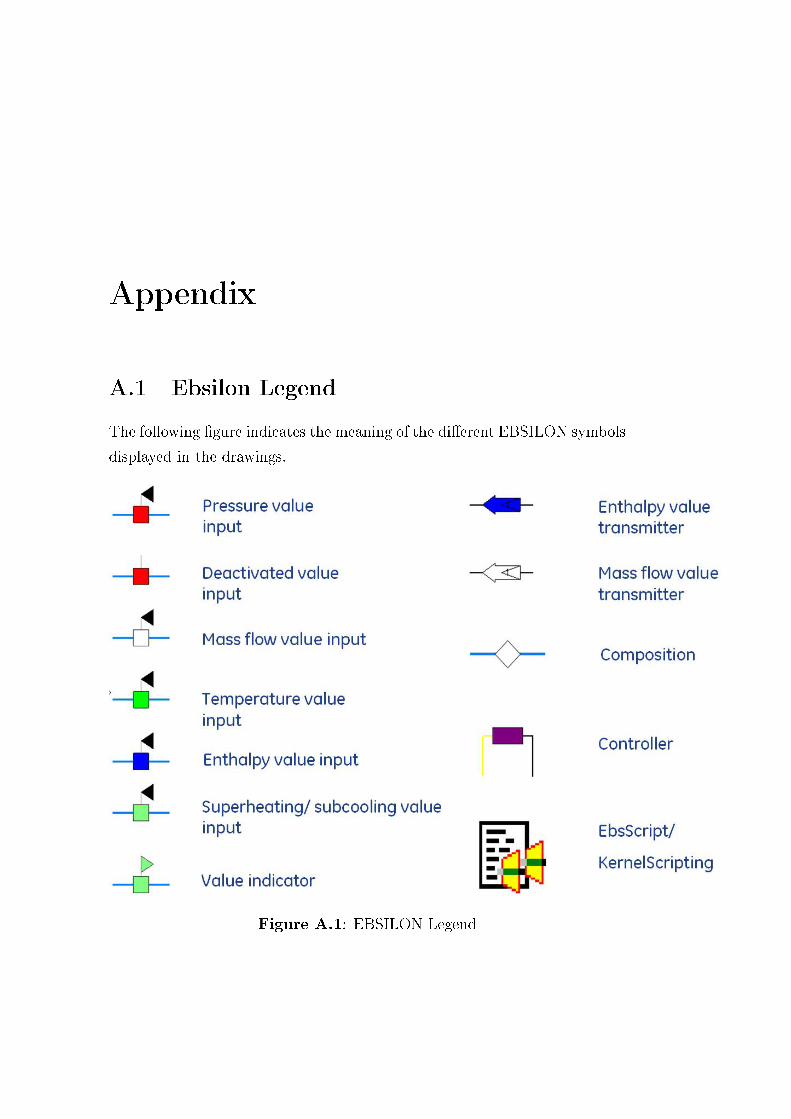
Appendix
A.1 Ebsilon Legend
The following �gure indicates the meaning of the di�erent EBSILON symbols
displayed in the drawings.
Figure A.1: EBSILON Legend
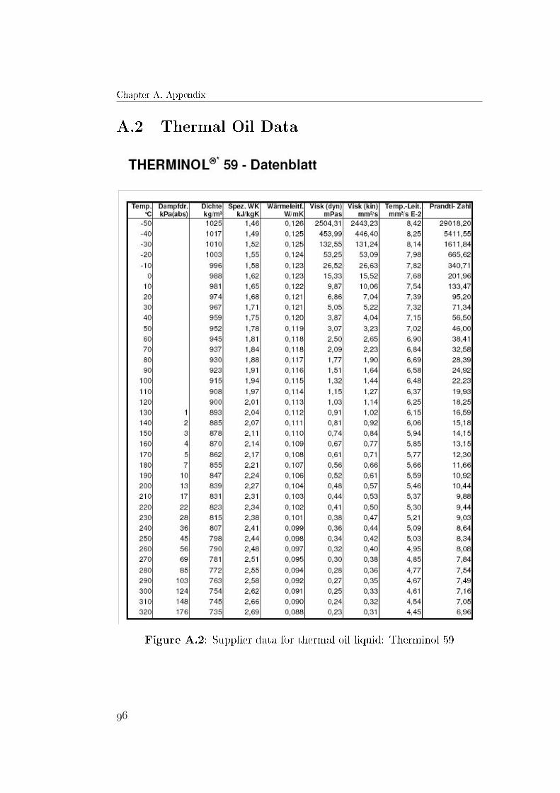
Chapter A. Appendix
A.2 Thermal Oil Data
Figure A.2: Supplier data for thermal oil liquid: Therminol 59
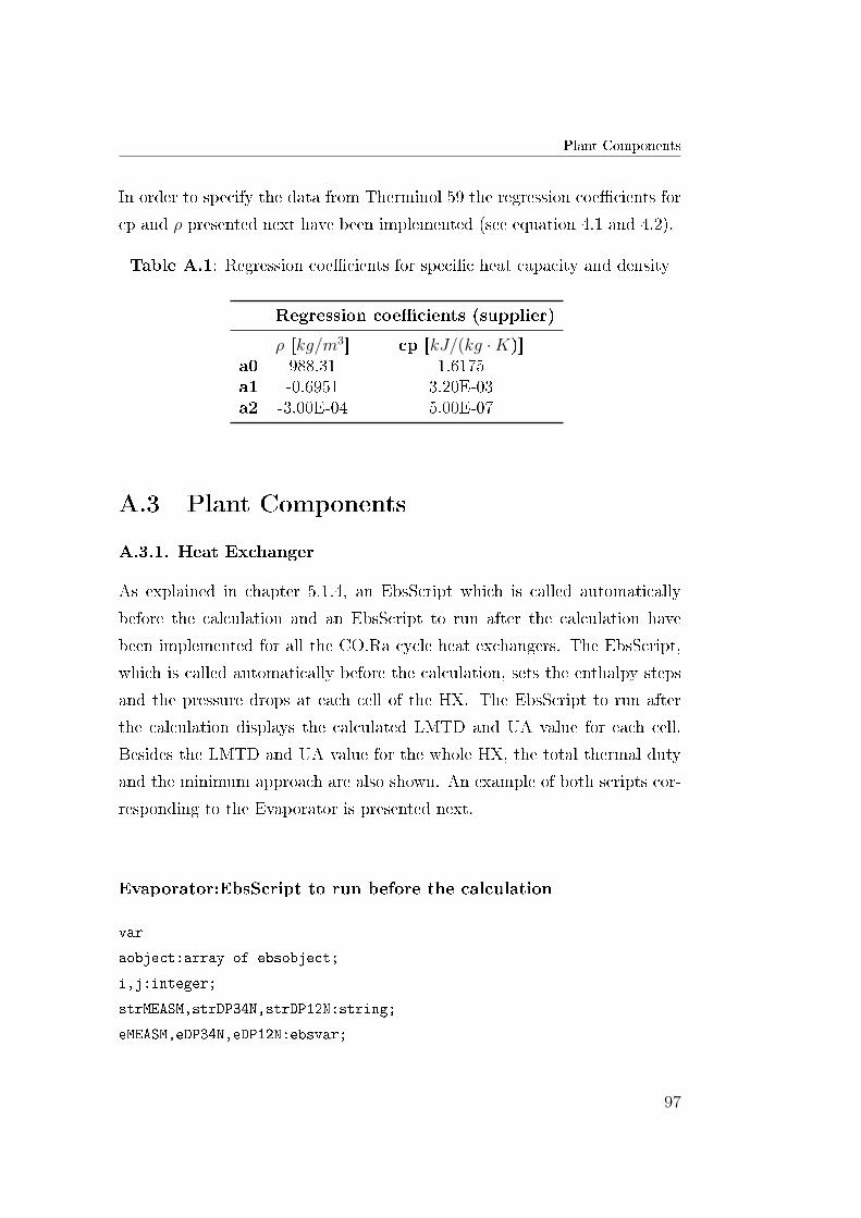
Plant Components
In order to specify the data from Therminol 59 the regression coe�cients for
cp and ρ presented next have been implemented (see equation 4.1 and 4.2).
Table A.1: Regression coe�cients for speci�c heat capacity and density
Regression coe�cients (supplier)
ρ [kg/m3] cp [kJ/(kg ·K)]a0 988.31 1.6175a1 -0.6951 3.20E-03a2 -3.00E-04 5.00E-07
A.3 Plant Components
A.3.1. Heat Exchanger
As explained in chapter 5.1.4, an EbsScript which is called automatically
before the calculation and an EbsScript to run after the calculation have
been implemented for all the CO.Ra cycle heat exchangers. The EbsScript,
which is called automatically before the calculation, sets the enthalpy steps
and the pressure drops at each cell of the HX. The EbsScript to run after
the calculation displays the calculated LMTD and UA value for each cell.
Besides the LMTD and UA value for the whole HX, the total thermal duty
and the minimum approach are also shown. An example of both scripts cor-
responding to the Evaporator is presented next.
Evaporator:EbsScript to run before the calculation
var
aobject:array of ebsobject;
i,j:integer;
strMEASM,strDP34N,strDP12N:string;
eMEASM,eDP34N,eDP12N:ebsvar;
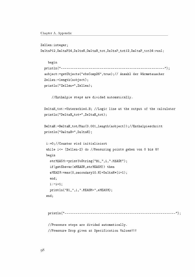
Chapter A. Appendix
Zellen:integer;
DeltaP12,DeltaP34,DeltaH,DeltaH_tot,DeltaP_tot12,DeltaP_tot34:real;
begin
println("--------------------------------------------------------");
aobject:=getObjects("ebsComp26",true);// Anzahl der Wärmetauscher
Zellen:=length(aobject);
println("Zellen=",Zellen);
//Enthalpie steps are divided automatically.
DeltaH_tot:=Unterschied.H; //Logic line at the output of the calculator
println("DeltaH_tot=",DeltaH_tot);
DeltaH:=DeltaH_tot/Max(0.001,length(aobject));//Enthalpieschritt
println("DeltaH=",DeltaH);
i:=0;//Counter wird initialisiert
while i<= (Zellen-2) do //Measuring points gehen von 0 bis 8!
begin
strMEASM:=printToString("H1_",i,".MEASM");
if(getEbsvar(eMEASM,strMEASM)) then
eMEASM:=max(0,secondary10.H)+DeltaH*(i+1);
end;
i:=i+1;
println("H1_",i,".MEASM=",eMEASM);
end;
println("------------------------------------------------------------");
//Pressure steps are divided automatically.
//Pressure Drop given at Specification Values!!!
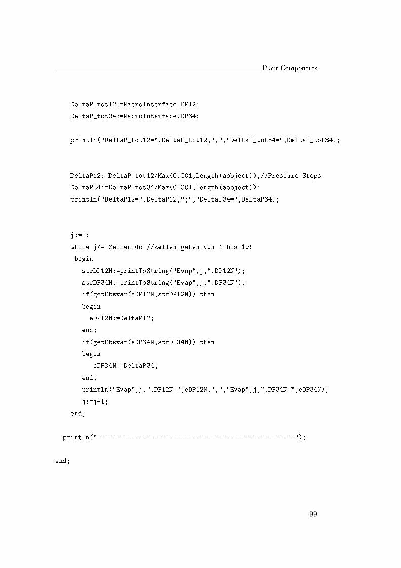
Plant Components
DeltaP_tot12:=MacroInterface.DP12;
DeltaP_tot34:=MacroInterface.DP34;
println("DeltaP_tot12=",DeltaP_tot12,",","DeltaP_tot34=",DeltaP_tot34);
DeltaP12:=DeltaP_tot12/Max(0.001,length(aobject));//Pressure Steps
DeltaP34:=DeltaP_tot34/Max(0.001,length(aobject));
println("DeltaP12=",DeltaP12,";","DeltaP34=",DeltaP34);
j:=1;
while j<= Zellen do //Zellen gehen von 1 bis 10!
begin
strDP12N:=printToString("Evap",j,".DP12N");
strDP34N:=printToString("Evap",j,".DP34N");
if(getEbsvar(eDP12N,strDP12N)) then
begin
eDP12N:=DeltaP12;
end;
if(getEbsvar(eDP34N,strDP34N)) then
begin
eDP34N:=DeltaP34;
end;
println("Evap",j,".DP12N=",eDP12N,",","Evap",j,".DP34N=",eDP34N);
j:=j+1;
end;
println("----------------------------------------------------");
end;
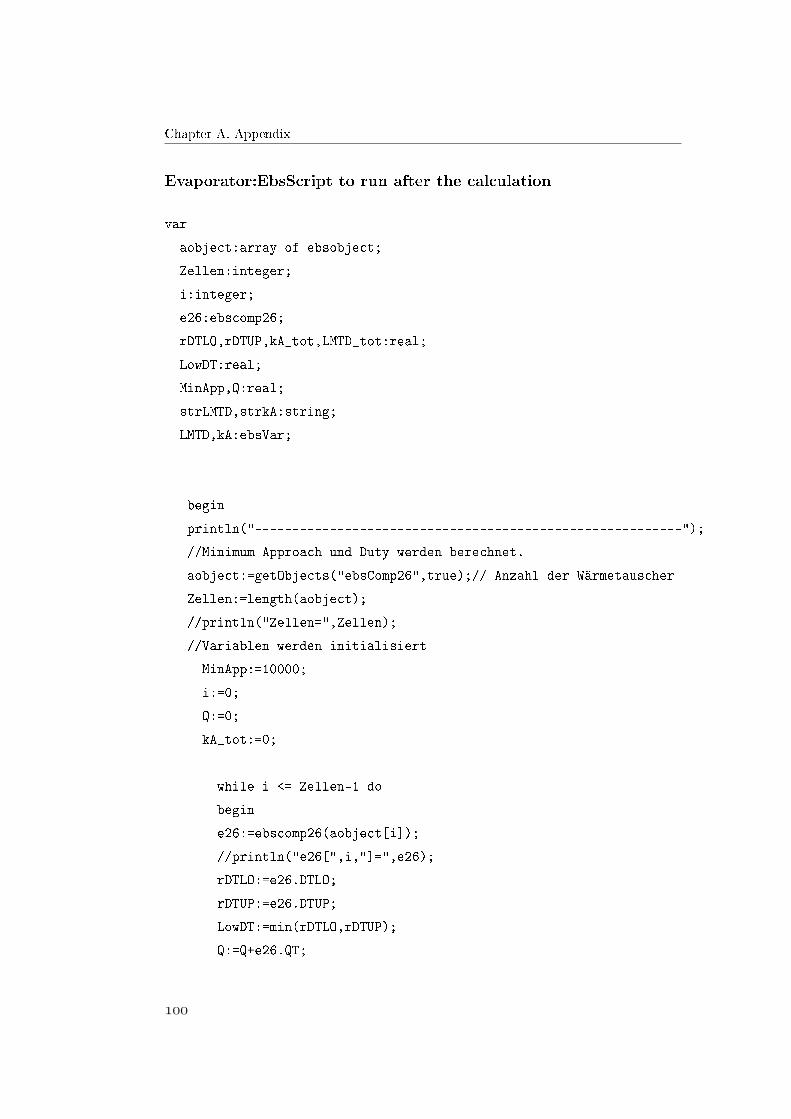
Chapter A. Appendix
Evaporator:EbsScript to run after the calculation
var
aobject:array of ebsobject;
Zellen:integer;
i:integer;
e26:ebscomp26;
rDTLO,rDTUP,kA_tot,LMTD_tot:real;
LowDT:real;
MinApp,Q:real;
strLMTD,strkA:string;
LMTD,kA:ebsVar;
begin
println("---------------------------------------------------------");
//Minimum Approach und Duty werden berechnet.
aobject:=getObjects("ebsComp26",true);// Anzahl der Wärmetauscher
Zellen:=length(aobject);
//println("Zellen=",Zellen);
//Variablen werden initialisiert
MinApp:=10000;
i:=0;
Q:=0;
kA_tot:=0;
while i <= Zellen-1 do
begin
e26:=ebscomp26(aobject[i]);
//println("e26[",i,"]=",e26);
rDTLO:=e26.DTLO;
rDTUP:=e26.DTUP;
LowDT:=min(rDTLO,rDTUP);
Q:=Q+e26.QT;

Plant Components
strLMTD:=printToString("Evap",i+1,".DTM");
strkA:=printToString("Evap",i+1,".kA");
getebsVar(LMTD,strLMTD);
getEbsVar(kA,strkA);
println("LMTD[Evap",i+1,"]=",LMTD,"; kA[Evap",i+1,"]=",kA);
kA_tot:=kA_tot+kA;
if LowDT<=MinApp then
MinApp:= LowDT;
i:=i+1;
end;
LMTD_tot:=Q/kA_tot;
println("-------------------------------------------------");
println("MinimumApproach=",MinApp);
println("Duty=",Q);
println("LMTD_tot=",LMTD_tot,"; kA_tot=",kA_tot);
println("---------------------------------------------------");
MacroInterface.Duty:=Q;
MacroInterface.LMTD:=LMTD_tot;
MacroInterface.UA:=kA_tot;
end;
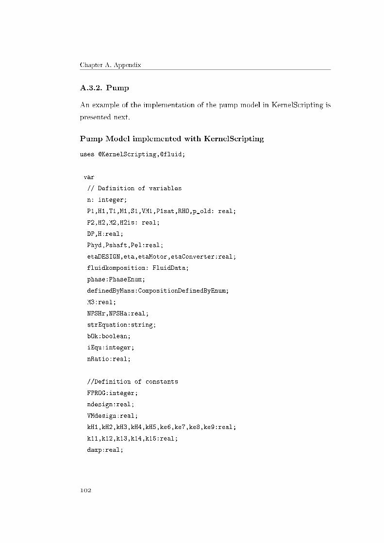
Chapter A. Appendix
A.3.2. Pump
An example of the implementation of the pump model in KernelScripting is
presented next.
Pump Model implemented with KernelScripting
uses @KernelScripting,@fluid;
var
// Definition of variables
n: integer;
P1,H1,T1,M1,S1,VM1,P1sat,RHO,p_old: real;
P2,H2,M2,H2is: real;
DP,H:real;
Phyd,Pshaft,Pel:real;
etaDESIGN,eta,etaMotor,etaConverter:real;
fluidkomposition: FluidData;
phase:PhaseEnum;
definedByMass:CompositionDefinedByEnum;
M3:real;
NPSHr,NPSHa:real;
strEquation:string;
bOk:boolean;
iEqu:integer;
nRatio:real;
//Definition of constants
FPROG:integer;
ndesign:real;
VMdesign:real;
kH1,kH2,kH3,kH4,kH5,ke6,ke7,ke8,ke9:real;
k11,k12,k13,k14,k15:real;
damp:real;

Plant Components
//-----------------------------------------------------------------
begin
FPROG:=ksGetFPROG;
println("FPROG=",FPROG);
//Receive inlet condition
P1:= ksGetPipeValue(1,PhysValueP);
M1:= ksGetPipeValue(1,PhysValueM);
H1:= ksGetPipeValue(1,PhysValueH);
println("P1=",P1,";","M1=",M1,";","H1=",H1);
//Table to calculate VM1 R245fa
ksGetPipeFluidData(1,fluidkomposition);
fluidTable( VM1,phase,P1,H1,FuncV_OF_PH,fluidkomposition,definedByMass );
//returns m3/kg
RHO:=1/max(0.0000001,VM1);
println("RHO=",RHO);
VM1:=VM1*M1;
println("VM1=",VM1);
p_old:= ksGetPipeValue(7,PhysValueP);
//-----------------------------------------------------------------
if FPROG=1 then begin
//Start Values
n:= ksGetPipeValue(2,PhysValueH);
//Regression equations characterisitc lines LT Pump
kH1,kH2,kH3,kH4,kH5,ke6,ke7,ke8,ke9,ndesign,nRatio: CONFIDENTIAL;
println ("n=",n," ndesign=",ndesign," nRatio=",nRatio);
VMdesign:= VM1*(ndesign/n)*(3600); // VMdesign in m3/h and VM1 in m3/s
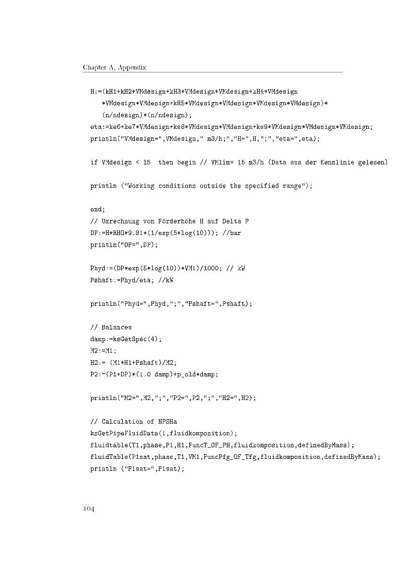
Chapter A. Appendix
H:=(kH1+kH2*VMdesign+kH3*VMdesign*VMdesign+kH4*VMdesign
*VMdesign*VMdesign+kH5*VMdesign*VMdesign*VMdesign*VMdesign)*
(n/ndesign)*(n/ndesign);
eta:=ke6+ke7*VMdesign+ke8*VMdesign*VMdesign+ke9*VMdesign*VMdesign*VMdesign;
println("VMdesign=",VMdesign," m3/h;","H=",H,";","eta=",eta);
if VMdesign < 15 then begin // VMlim= 15 m3/h (Data aus der Kennlinie gelesen)
println ("Working conditions outside the specified range");
end;
// Umrechnung von Förderhöhe H auf Delta P
DP:=H*RHO*9.81*(1/exp(5*log(10))); //bar
println("DP=",DP);
Phyd:=(DP*exp(5*log(10))*VM1)/1000; // kW
Pshaft:=Phyd/eta; //kW
println("Phyd=",Phyd,";","Pshaft=",Pshaft);
// Balances
damp:=ksGetSpec(4);
M2:=M1;
H2:= (M1*H1+Pshaft)/M2;
P2:=(P1+DP)*(1.0-damp)+p_old*damp;
println("M2=",M2,";","P2=",P2,";","H2=",H2);
// Calculation of NPSHa
ksGetPipeFluidData(1,fluidkomposition);
fluidtable(T1,phase,P1,H1,FuncT_OF_PH,fluidkomposition,definedByMass);
fluidTable(P1sat,phase,T1,VM1,FuncPfg_OF_Tfg,fluidkomposition,definedByMass);
println ("P1sat=",P1sat);

Plant Components
NPSHa:=(P1-P1sat)*exp(5*log(10))*(VM1/M1)/9.81;
println ("NPSHa=",NPSHa);
// Calculation of NPSHr
k11,k12,k13,k14,k15:=CONFIDENTIAL;
NPSHr:=(k11+k12*VMdesign+k13*VMdesign*VMdesign+k14*VMdesign*VMdesign*VMdesign+
k15*VMdesign*VMdesign*VMdesign*VMdesign)*(n/ndesign)*(n/ndesign);
println ("Low NPSHr=",NPSHr);
if NPSHa < NPSHr then begin
println ("Atention!Cavitation problem!");
end;
println("---------------------------------------------------");
///Set Outlet Streams
ksRemoveAllEquations;
iEqu:=1;
strEquation:=printToString("M1-M7=0");
bOk:=ksSetEquation(iEqu,strEquation);
iEqu:=iEqu+1;
strEquation:=printToString("P7=",P2);
bOk:=ksSetEquation(iEqu,strEquation);
iEqu:=iEqu+1;
strEquation:=printToString("H7=",H2);
bOk:=ksSetEquation(iEqu,strEquation);
iEqu:=iEqu+1;
ksSetRES (1,eta);
end
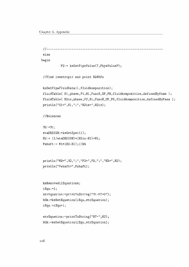
Chapter A. Appendix
//-----------------------------------------------------------------
else
begin
P2:= ksGetPipeValue(7,PhysValueP);
//Find isentropic end point R245fa
ksGetPipeFluidData(1,fluidkomposition);
fluidTable( S1,phase,P1,H1,FuncS_OF_PH,fluidkomposition,definedByMass );
fluidTable( H2is,phase,P2,S1,FuncH_OF_PS,fluidkomposition,definedByMass );
println("S1=",S1,";","H2is=",H2is);
//Balances
M2:=M1;
etaDESIGN:=ksGetSpec(1);
H2:= (1/etaDESIGN)*(H2is-H1)+H1;
Pshaft:= M1*(H2-H1);//kW
println("M2=",M2,";","P2=",P2,";","H2=",H2);
println("Pshaft=",Pshaft);
ksRemoveAllEquations;
iEqu:=1;
strEquation:=printToString("M1-M7=0");
bOk:=ksSetEquation(iEqu,strEquation);
iEqu:=iEqu+1;
strEquation:=printToString("H7=",H2);
bOk:=ksSetEquation(iEqu,strEquation);
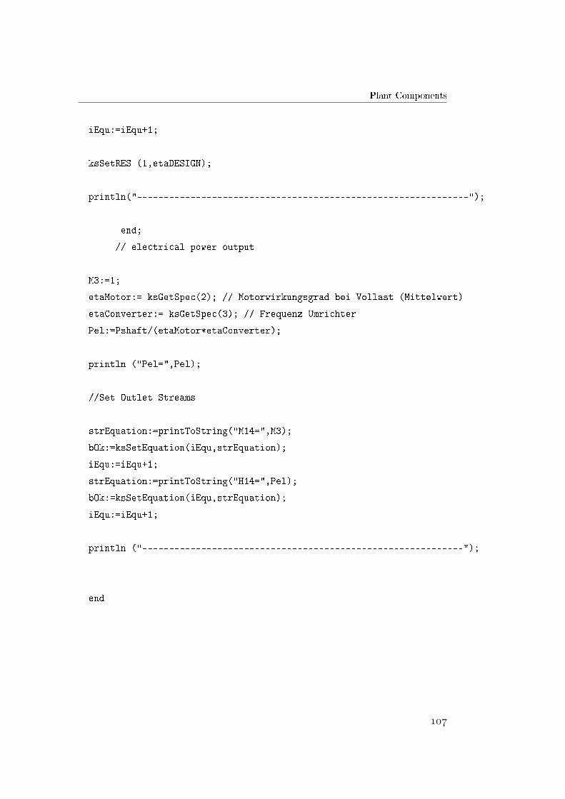
Plant Components
iEqu:=iEqu+1;
ksSetRES (1,etaDESIGN);
println("--------------------------------------------------------------");
end;
// electrical power output
M3:=1;
etaMotor:= ksGetSpec(2); // Motorwirkungsgrad bei Vollast (Mittelwert)
etaConverter:= ksGetSpec(3); // Frequenz Umrichter
Pel:=Pshaft/(etaMotor*etaConverter);
println ("Pel=",Pel);
//Set Outlet Streams
strEquation:=printToString("M14=",M3);
bOk:=ksSetEquation(iEqu,strEquation);
iEqu:=iEqu+1;
strEquation:=printToString("H14=",Pel);
bOk:=ksSetEquation(iEqu,strEquation);
iEqu:=iEqu+1;
println ("------------------------------------------------------------");
end
Chapter A. Appendix
A.3.3. Turbine
In order to calculate the o�-design behaviour of the turbine, an empirical
model has been developed to calculate the mass �ow and the e�ciency. This
model has been created with KernelScripting.
Turbine Empirical Model implemented with KernelScripting
uses @KernelScripting,@fluid;
var
// Definition of variables
n: real;
P1,H1,T1,M1,S1: real;
P2,H2,M2,H2is: real;
nRed,mRed: real;
Eta,etaDESIGN: real;
fluidkomposition: fluidData;
phase:PhaseEnum;
definedByMass:CompositionDefinedByEnum;
//Definition of constants
FPROG:integer;
ndesign:real;
km1,km2,km3,km4,km5,km6,km7,km8,km9:real;
kEta1,kEta2,kEta3,kEta4,kEta5,kEta6,kEta7,kEta8,kEta9:real;
begin
// Regression constants
km1,km2,km3,km4,km5,km6,km7,km8,km9,kEta1,kEta2,kEta3,kEta4,kEta5,
kEta6,kEta7,kEta8,kEta9:=CONFIDENTIAL;
//ONDesign or OFFDesign Modus?

Plant Components
FPROG:=ksGetFPROG;
println("FPROG=",FPROG);
//Receive inlet conditions
P1:= ksGetPipeValue (2,PhysValueP); //index 2: entry pipe
H1:= ksGetPipeValue (2,PhysValueH);
P2:= ksGetPipeValue (1,PhysValueP); //index 1:exit pipe
println("P1=",P1,";","H1=",H1,";","P2=",P2);
//Table to calculate T1 cyclohexane/R245fa
ksGetPipeFluidData(2,fluidkomposition);
fluidTable( T1,phase,P1,H1,FuncT_OF_PH,fluidkomposition,definedByMass);
println("T1=",T1);
//Find isentropic end point R245fa
ksGetPipeFluidData(2,fluidkomposition);
fluidTable( S1,phase,P1,H1,FuncS_OF_PH,fluidkomposition,definedByMass);
fluidTable( H2is,phase,P2,S1,FuncH_OF_PS,fluidkomposition,definedByMass);
println("S1=",S1,";","H2is=",H2is);
//------------------------------------------------------------------------
if FPROG=1 then //Off Design Modus: Efficiency and massflow calculated
begin
//Start values
n:= ksGetPipeValue(4,PhysValueH);
println("n=",n);
ndesign:=ksGetSpec(1); //ndesign=22800 (Wert aus Dymola)
println("ndesign=",ndesign);
//Warning if we are outside the margins where the regression is valid!
//if (n > = 10800 and n < = 25800) then OK
Chapter A. Appendix
//if (P1/P2)> 1,939 and (P1/P2) < 3,383 then OK
if (n < 10800 or n > 25800) then
println("REGRESSION NOT VALID(Rotary Speed outside the margins)!");
if ( (P1/P2)<=1.939 or (P1/P2)>=3.383) then
println("REGRESSION NOT VALID(Pressure Ratio outside the margins)!");
//Definiton of auxiliary equations(regression model)
nRed:=(n/(sqrt((T1+273.15))));
mRed:=km1+km2*(P1/P2)+km3*nRed+km4*nRed*(P1/P2)+
km5*(P1/P2)*(P1/P2)+ km6*nRed*nred+km7*(P1/P2)*(P1/P2)*(nRed)
+ km8*nRed*nRed*(P1/P2)+km9*(P1/P2)*(P1/P2)*(P1/P2);
Eta:=kEta1+kEta2*(nRed)+kEta3*(P1/P2)+kEta4*(nRed)*(P1/P2)+
kEta5*(nRed)*(nRed)+
kEta6*(P1/P2)*(P1/P2)+kEta7*(nRed)*(nRed)*(P1/P2)+
kEta8*(P1/P2)*(P1/P2)*(nRed)+
kEta9*(P1/P2)*(P1/P2)*(P1/P2);
println("nRed=",nRed,";","mRed=",mRed,";","Eta=",Eta);
//Definition of main equations (Balances)
M1:=mRed*P1*100000/(sqrt((T1+273.15))); //Umrechung Druck auf Pascal
H2:= H1-(H1-H2is)*Eta;
//Electrical Power is calculated with component 11 (Generator)
//If we take away the generator:
//Pshaft:= M1*(H2-H1);
//Pel:=etaConverter*etaGen*Pshaft; etaConverter 0,97; etaGenerator 0,95.
println("M1=",M1,";","Eta=",Eta,";","H2=",H2);
println("-------------------------------------------------------------");
Plant Components
//Results OFFDESIGN MODUS
ksSetPipeValue(12,PhysValueM,M1);
ksSetPipeValue(14,PhysValueH,H2);
ksSetRes(1,M1);
ksSetRes(2,H2);
ksSetRes(3,Eta);
end;
//----------------------------------------------------------------------
if FPROG=0 then //ON Design Modus: Eta and massflow given.
begin
M1:=ksGetPipeValue(2,PhysValueM);
etaDESIGN:=ksGetSpec(2);
H2:= H1-(H1-H2is)*etaDESIGN;
println("M1=",M1,";","etaDESIGN=",etaDESIGN,";","H2=",H2);
println("----------------------------------------------------------------");
//Results ON DESIGN MODUS
ksSetPipeValue(14,PhysValueH,H2);
ksSetRes(1,M1);
ksSetRes(2,H2);
ksSetRes(3,etaDESIGN);
end
end;