
Development of an XFEM based Adaptive Contact Model for ...
104
TECHNISCHE UNIVERSITÄT MÜNCHEN Lehrstuhl für Angewandte Mechanik Development of an XFEM based Adaptive Contact Model for Telepresence Systems with Time Delay Keita Ono Vollständiger Abdruck der von der Fakultät für Maschinenwesen der Technischen Universität München zur Erlangung des akademischen Grades eines Doktor-Ingenieurs genehmigten Dissertation. Vorsitzender: Univ.-Prof. Dr.-Ing. Gunther Reinhart Prüfer der Dissertation: 1. Univ.-Prof. Dr.-Ing. Dr.-Ing. habil. Heinz Ulbrich 2. Univ.-Prof. Dr.-Ing. habil. Bodo Heimann (i.R.) Leibniz Universität Hannover Die Dissertation wurde am 05.07.2011 bei der Technischen Universität München eingereicht und durch die Fakultät für Maschinenwesen am 09.11.2011 angenommen.
Transcript of Development of an XFEM based Adaptive Contact Model for ...

TECHNISCHE UNIVERSITÄT MÜNCHENLehrstuhl für Angewandte Mechanik
Development of an XFEM basedAdaptive Contact Modelfor Telepresence Systems
with Time Delay
Keita Ono
Vollständiger Abdruck der von der Fakultät für Maschinenwesen der
Technischen Universität München zur Erlangung des akademischen Grades eines
Doktor-Ingenieurs
genehmigten Dissertation.
Vorsitzender:
Univ.-Prof. Dr.-Ing. Gunther Reinhart
Prüfer der Dissertation:
1. Univ.-Prof. Dr.-Ing. Dr.-Ing. habil. Heinz Ulbrich
2. Univ.-Prof. Dr.-Ing. habil. Bodo Heimann (i.R.)Leibniz Universität Hannover
Die Dissertation wurde am 05.07.2011 bei der Technischen Universität München
eingereicht und durch die Fakultät für Maschinenwesen am 09.11.2011 angenommen.
Contents
Abstract III
1 Introduction 11.1 Problem statements and research focuses . . . . . . . . . . . . . . . . 21.2 Aspects and outline . . . . . . . . . . . . . . . . . . . . . . . . . . . . 3
2 Contact model for time delay in a medical telepresence system 52.1 Medical telepresence system . . . . . . . . . . . . . . . . . . . . . . . 52.2 Telepresence system and time delay . . . . . . . . . . . . . . . . . . . 62.3 Contact model and model based control . . . . . . . . . . . . . . . . 7
2.3.1 Smith predictor . . . . . . . . . . . . . . . . . . . . . . . . . . 72.3.2 Time delay compensation . . . . . . . . . . . . . . . . . . . . 82.3.3 Modeling of incision in soft body . . . . . . . . . . . . . . . . 92.3.4 Family of finite element methods . . . . . . . . . . . . . . . . 9
3 Incision mechanics in a soft body 123.1 Definition of a cut in a solid body . . . . . . . . . . . . . . . . . . . . 123.2 Kinematics . . . . . . . . . . . . . . . . . . . . . . . . . . . . . . . . 13
3.2.1 Deformation . . . . . . . . . . . . . . . . . . . . . . . . . . . . 133.2.2 Material structural and spatial configurational changes . . . . 153.2.3 Deformation gradient . . . . . . . . . . . . . . . . . . . . . . . 153.2.4 Stress and strain . . . . . . . . . . . . . . . . . . . . . . . . . 163.2.5 Constitutive equations . . . . . . . . . . . . . . . . . . . . . . 17
3.3 Conservation of momentum . . . . . . . . . . . . . . . . . . . . . . . 183.4 Boundary value problems . . . . . . . . . . . . . . . . . . . . . . . . . 19
3.4.1 Initial value problems . . . . . . . . . . . . . . . . . . . . . . . 213.5 Remapping of the governing system of equations . . . . . . . . . . . . 213.6 Weak form of conservation of momentum . . . . . . . . . . . . . . . . 22
3.6.1 Strong to weak form . . . . . . . . . . . . . . . . . . . . . . . 233.6.2 Smoothness of the test function and the trial function . . . . . 243.6.3 Principle of virtual work . . . . . . . . . . . . . . . . . . . . . 24
4 Finite element approach 264.1 Spatial discretization . . . . . . . . . . . . . . . . . . . . . . . . . . . 264.2 Discrete governing system of equations . . . . . . . . . . . . . . . . . 284.3 Element coordinates . . . . . . . . . . . . . . . . . . . . . . . . . . . 304.4 Assembly and remeshing . . . . . . . . . . . . . . . . . . . . . . . . . 32
4.4.1 Assembly process . . . . . . . . . . . . . . . . . . . . . . . . . 324.4.2 Remeshing . . . . . . . . . . . . . . . . . . . . . . . . . . . . . 33
I
Contents II
4.5 Dynamic simulation . . . . . . . . . . . . . . . . . . . . . . . . . . . . 344.5.1 Newmark implicit integration . . . . . . . . . . . . . . . . . . 344.5.2 Solution of linear algebraic equations . . . . . . . . . . . . . . 36
4.6 Implementation . . . . . . . . . . . . . . . . . . . . . . . . . . . . . . 37
5 Extended finite element approach 415.1 Displacement approximation with discontinuities . . . . . . . . . . . . 425.2 Modeling of strong discontinuous fields . . . . . . . . . . . . . . . . . 43
5.2.1 Heaviside function . . . . . . . . . . . . . . . . . . . . . . . . 445.2.2 Shifted function . . . . . . . . . . . . . . . . . . . . . . . . . . 44
5.3 Discrete governing system of equations with XFEM . . . . . . . . . . 475.4 Enrichment nodes selection and assembly . . . . . . . . . . . . . . . . 51
5.4.1 Enrichment nodes selection . . . . . . . . . . . . . . . . . . . 515.4.2 Assembly of enrichment DoFs . . . . . . . . . . . . . . . . . . 52
5.5 Dynamic simulation . . . . . . . . . . . . . . . . . . . . . . . . . . . . 535.6 Implementation . . . . . . . . . . . . . . . . . . . . . . . . . . . . . . 53
6 Remarks on implementation practicality 576.1 Finite element method with remeshing . . . . . . . . . . . . . . . . . 576.2 Extended finite element method . . . . . . . . . . . . . . . . . . . . . 586.3 Discussion on the practicality . . . . . . . . . . . . . . . . . . . . . . 59
7 Adaptive empirical incision force model 617.1 Force modeling of haptic incision perception . . . . . . . . . . . . . . 61
7.1.1 Friction on lubricated surface . . . . . . . . . . . . . . . . . . 627.1.2 Incision force model in Cartesian system . . . . . . . . . . . . 63
7.2 Adaptive parameter identification . . . . . . . . . . . . . . . . . . . . 667.3 Optimization . . . . . . . . . . . . . . . . . . . . . . . . . . . . . . . 727.4 Implementation of the adaptive contact model . . . . . . . . . . . . . 73
8 Experiments and results 768.1 Experimental telepresence system . . . . . . . . . . . . . . . . . . . . 76
8.1.1 Teleoperator . . . . . . . . . . . . . . . . . . . . . . . . . . . . 788.1.2 Tension platform . . . . . . . . . . . . . . . . . . . . . . . . . 798.1.3 Test object . . . . . . . . . . . . . . . . . . . . . . . . . . . . 808.1.4 Software framework . . . . . . . . . . . . . . . . . . . . . . . . 81
8.2 Time delay compensation utilizing contact model . . . . . . . . . . . 828.2.1 Impact of time delay during incision . . . . . . . . . . . . . . 838.2.2 Incision force compensation utilizing contact model . . . . . . 86
9 Conclusion and future works 909.1 Discussion . . . . . . . . . . . . . . . . . . . . . . . . . . . . . . . . . 909.2 Outlooks . . . . . . . . . . . . . . . . . . . . . . . . . . . . . . . . . . 91
A Mechanical properties of silicone 93
Bibliography 94
Abstract
An incision is a common process in medical telepresence applications. When a largedistance between the human operator and the teleoperator is presented, it can leadto a time delay in communication channel which causes the hand’s movement and theforce feedback perception not to synchronize. This research work proposed an adap-tive contact model based on the Extended Finite Element Method. The proposedcontact model compensates the time delay using the real-time dynamic geometry de-formation simulation and the calculation of the corresponding incision force betweenthe scalpel at the end-effector of the teleoperator and the remote environment. Anadaptive parameter identification algorithm is also developed allowing online modelverification during the actual incision. The experimental results demonstrate a sta-bility improvement during the incision with the experimental telepresence system.
Keywords: Telepresence system, Extended Finite Element Method (XFEM), Real-time Incision simulation, Adaptive control, Mechatronics
Kurzfassung
In medizinischen Telepräsenzanwendungen können bei großer Entfernung zwischenOperator und Teleoperator Zeitverzögerungen in der Kommunikation dazu führen,dass die Handbewegungen des Operators und die Kraftrückkopplung vom Kraftsen-sor nicht synchron sind. Zur Lösung des Problems wird ein Kontaktmodell ent-worfen, das auf der Extended Finite Element Methode basiert. Mit diesem Kon-taktmodells ist es möglich die dynamische Verformung eines weichen Kontaktes zusimulieren und die Kraftrückkopplung während des Schnittes in Echtzeit zu berech-nen und auszugeben. Dadurch bleibt die Synchronisation zwischen der Operatorbe-wegung und der Kontaktkraftwahrnehmung erhalten. Zusätzlich wird ein adaptiverParameteridentifikationsalgorithmus entwickelt und mit dem Kontaktmodell gekop-pelt. Damit wird eine Modellverifizierung in Echtzeit ermöglicht und gegebenenfallseine Adaption der Modellparametereinstellung während der Teleoperation durchge-führt.
Stichworte: Telepräsenzsystem, Extended Finite Elemente Methode (XFEM), Echtzeit-simulation eines Schneidevorgangs, Adaptivregelung, Mechatronik
III

1 Introduction
The advancements in engineering and information technologies keep opening newpossibilities to the robotic researchers. Therefore, the robotic technology has beenevolving in recent years to cover numerous of applications. As one of an importantrobotic research field, the telerobotic benefits directly from the modern communica-tion technologies allowing a robotic system to be controlled from another location.The telepresence system belongs to the telerobotic category but differentiate itselfby a distinguish and control method.
The concept of telepresence and often including teleaction [48] comprises with theessential components which are a human operator, a control devices, a teleoperatorand a remote environment which is sensed and acted upon by the teleoperator [41].The control devices of a telepresence system can be called a human-robot controlinterface [34]. A simplified schematic outline of a telepresence system is presentedin Figure 1.1.
Delayed Communication
InputSignals
FeedbackSignals
Teleoperator
Force Sensor
Camera System
Microphone
Human Operator
Haptic Device
Visualization
Audio Feedback
Local Station
Rem
ote Environment
Figure 1.1: A schematic of a multimodal telepresence system, adapted from [65]
A telepresense system employs a bilateral control scheme in order to provide a hu-man operator a virtual but realistic access to a remote environment at distance.The devices used as the control interface, for instances, a haptic device, a head-mounted display and a three-dimensional audio feedback are generally mapped tothe corresponding sensor arrays of the teleoperator in the remote environment. Theadvantage of a telepresence system is that the existing of the human operator inthe same location of the robotic system may not be necessary. The control interfacecan be intuitive and connected to the sensorial system of a human operator. Which
1
1.1 Problem statements and research focuses 2
means that this human operator is associated with the teleoperator system in theremote environment via a network infrastructure and interactively manipulates theremote environment with dexterity relying on the feedback signals. Because of itscontrol interface, the telepresence allows theoretically a human operator to transfertheir particular skill to the robotic system. It can be alleged that if the telepresenceexperience is natural or transparent to a human operator completely, the rate ofsuccess in the given task shall solely depend on their skill factors. The ideal telep-resence is often described as an immersive experience of the human operator intothe remote environment with all his or her sensory abilities.
Telepresence systems are involving in different areas of applications. For a shortexample: the space exploration and on-orbit service, the ROKVISS of the Ger-man Aerospace Center [50, 69] and the Robonaunt of NASA [47], medical treat-ments [44, 53, 64], plant maintenance and assembly [22, 70]. The researchers in thisarea have not been being challenged only to overcome technical limitation of thesystem implementation but also forced to encounter a requirement of producing areliable robotic system.
As an example, Collaborative Research Centre 453 (SFB 453) High-Fidelity Telep-
resence and Teleaction (1998-2010), financially supported by the German Research
Foundation (DFG) was appointed particularly to explore the possibilities and de-velop new technologies of the telepresence applications in numerous branches ofareas [1].
1.1 Problem statements and research focuses
An important characteristic of a telepresence system is the distance between theteleoperator and its human operator. This advantage is a self-contradictory sinceit may lead to a time delay in the communication channel. A time delay existsin each communication medium and, if significant, is one of major causes to thefailure of telepresence system causing the loss of the synchronization between theinput commands and the feedback perceptions. To solve this technical problem, thisresearch work, under subproject M7 of SFB 453, proposed the principle of contactmodel to compensate the time delay in the communication. A contact model isrequired to substitute the actual delayed feedback visualization and the contactforce perception with the results from a real-time simulation.
The contact model developed in this work focuses specifically on the incision pro-cess in a soft body with a scalpel common for the medical telepresence applications.To achieve a real-time graphic visualization simulation, a dynamic geometry defor-mation of the soft body must be demonstrated. Two approaches, Finite ElementMethod (FEM) and Extended Finite Element Method (XFEM) are investigated.The calculation of the contact force between a scalpel and the soft body is doneusing the empirical incision force model.

1.2 Aspects and outline 3
Additionally, the usability of the contact model is enhanced by the introduction ofan adaptive parameter identification algorithm. The algorithm allows the contactmodel to be verified online during the actual incision is being carried out by theteleoperator.
1.2 Aspects and outline
To achieve this research focuses, the outline of this work is systematically designedto open essential discussions related to the topic while providing an answer to eachdiscussion from the development of the proposed adaptive contact model to theconclusion of the results.
To begin with, Chapter 2 is developed to provide an overview of the primary problemfor a medical telepresence system regarding time delay. The essential engineeringconcepts and principles employed in the development will be presented along withthe introductory notes on important technical definitions with their related workscommonly referred in this specific area of applications.
Chapter 3 will extensively discuss on the physical interpretation of the incisionmechanics using the theory of continuum mechanics. The material and structuralchanges due to the evolution of the incision will be considered. The investigationin this chapter provides the linear governing system of equations necessary for thedynamic simulation of the geometry deformation of a soft body subjected to inci-sion.
To achieve a real-time simulation of the geometry deformation, the derived lineargoverning system of equations is discretized using FEM in Chapter 4. A discussionon the remeshing algorithm required to update the governing system of equationscorresponding to the cut evolution will be made. Chapter 5 is devoted to XFEMwhich is the second approach employed to discrete the governing system of equationsderived in Chapter 3. The demonstration of a cut evolution by XFEM in term of amathematic approximation will be presented and discussed.
FEM and XFEM approaches are investigated in this work as a implementation toolfor a contact model for incision process. It is critical that the approach should bepractical and flexible for implementation a different physical aspects of the unfa-miliar remote environment. In Chapter 6, the evaluation on this matter will bespecifically made.
The development of an empirical incision force model is demonstrated in Chap-ter 7 along with its adaptive parameter identification algorithm. Additionally, theoptimization employed to the performance of the incision force model the will bepresented.
In chapter 8, the results of the impact of time delay to the test object during anincision will be presented in comparison with the results of the same incision process

1.2 Aspects and outline 4
while utilizing the proposed adaptive contact model. Chapter 9 concludes the resultswith related discussions and outlooks.
2 Contact model for time delay in a medicaltelepresence system
This chapter is aimed to provide an overview of topics related to the problem state-ments and the focuses of this work. The chapter will begin with a brief introductionof the medical telepresence system before concentrates on a problem of time delay inthe communication. The principle and benefits of contact model will be discussedin terms of classical control theory as a feasible solution to time delay problem.The theory of continuum mechanics and Finite Element Methods employed in thiswork as development tools of the contact model for an incision process will be alsodiscussed.
2.1 Medical telepresence system
There are many telepresence systems developed not only allowing skill transfer froma human operator to the machine but also to enhance and improve the performancebeyond their ordinary abilities. Particularly in medical area, a robot based surgeryis one of major interests of many telepresence developers. A medical telepresencesystem is generally designed so that the surgeon can handle the same operation usingtheir individual skills and techniques. The ultimate goal in medical telerobotic isto allow a surgeon to provide his medical expertises to a patient independent fromlocation.
It is however a fact that the current generation of telepresence systems do not yetprovide an ideal and transparent telepresence experiences to their operators. Thisis generally because the different in physical of the robot manipulators and humanarms with the control interface. Therefore, a direct skill transfer from a human tomachine can not be easily achieved. The researchers take an effort to develop thesupplemental systems helping the operators to overcome the limit or unfamiliarityof the control interface. For example, Tavakoli et al. investigates the different injoint impedances between the control interface and the teleoperator manipulator oftheir Zeus medical robot system. They proposed a sensor which measures the veloc-ity of the robot end-effector and accordingly calculates a compensation force at theoperator’s side which matches their impedances [90]. Hirzinger et al. developsMiroSurge aiming for heart surgery capable of automatic manipulator compensationfor heart-beating movement [44].
The control interface of the telepresence system may not be intuitive enough insome cases for its human operator to undergone a complicate task-handling. Thus,
5
2.2 Telepresence system and time delay 6
the automatic routine task-handling and the visual guidance control algorithms isintensively studied by Mayer and Staub to support and ease the learning-curveof a human operator. The algorithms provides aid to the operator with an semi-automatic sequence by knot-typing [53,87].
Some of development criteria are not focusing on the performance enhancementalone, but also pursuing to maintain or improve the usability and efficiency of thetelepresence system. For instance, time delay in communication channel can reducethe level of fidelity of the telepresence system and prevent the operation to be carriedout successfully. The main focus of this work stays in this particular category.
2.2 Telepresence system and time delay
In some telepresence systems, a technical limit such as large time delay in com-munication is inevitable. Significant time delay occurs if the distance between thehuman operator and the teleoperator is large or a communication protocol withinefficient transmission rate is involved. The time delay in a telepresence systemcauses a postpone arrival of the input and feedback signals. This causes the level ofsynchronization between these signals to be declined. Because the telepresence sys-tem is controlled by human operators and relying on their perceptions, the humanoperators may react to the false feedback perception. In a severe case, the remoteenvironment and the teleoperator can be damaged. It is difficult to justify the maxi-mum amount of time delay which still allows the telepresence operation to be safelyexecuted. It depends strongly on the individual application, hardware design andforemost, human factors. As a guide line quoted by Held and Sheridan, 300msis often referred as a maximum allowance [41,76].
Most of the current telepresence systems require an individual communication chan-nel, e.g. over satellite or fiber optic cable. However, the approach only promisesthe communication will not be interrupted easily by an unforeseen transmissions.Thus, the data transfer rate should be stable as far as the physical limits of thenetwork can provide. On the other hand, Eckehard proposes one of a logical stepto increase the stability by reducing the amount of transmitted data [88]. However,in random situations where the data are completely lost due to an interruption incommunication, the reduction of data may cause a severe damage since the reducedor compressed data by the algorithm may contain valuable information. The prin-ciple of wave variable is one another well-known method employed in many currenttelepresence systems to especially cope with the time delay problem. Example im-plementations on this topic can be referred by the works of Slotine et al. [82,83],Hirsche et al. [42, 43] also Smith et al. [84]. This principle alters both inputand output variables transmitted fort and back between operator and the teleopera-tor to guarantee a certain level of synchronization between the feedback perceptionand the actual movement of the teleoperator. However, its effect may conduct an

2.3 Contact model and model based control 7
unrealistic telepresence experience due to the incorrect rendering of the actual con-tact behavior. For this reason, the principle of wave variable may not suitable for atelepresence scenario such as medical teleoperation involving incision process.
The second fact about time delay demonstrated by Mitsuishi is its dependency onthe physical distance between the operator and the teleoperator comprising the net-working and individual equipments used [55]. It is also true that networking requiredmany levels of data synchronizations and package loss are common. Shorter physicaldistance and less number of medium equipments are definitely preferred. In mostcase, time delay is treated as a property of the system. It should be known at handbefore initiating a telepresence system. Consider the impracticality of reserving asatellite communication channel or adapt the communication protocol including itsnetworking equipments, the ideal communication sufficient for a transparent telep-resence experience to the operator can be questionable.
2.3 Contact model and model based control
2.3.1 Smith predictor
In a classical control, the time delay problem has been addressed for decades. Alarge time delay in a control loop is seen frequently in many process control applica-tions, such as a chemical process in which a real-time monitoring of actual chemicalreaction is often not feasible. With a time delay existing between the plant and thecontroller, the gain-margin and phase-margin are decreased. It is up to the plantdynamic when should the system goes instable. The actual causes depend on theprocess itself and partly due to sensor limitations. In other words, the monitoringof the state of the process can not be measured physically due to a sub-reactionwith a large time-constant prohibits a proper measurement of the actual state ofthe process before the control substance reaches the sensitivity range of the sensor.larger the time delay is, will the system more likely be unstable. This phenomenonis comparable, in case of a telepresence system, to the delay of data arrival and datalost in its communication channel, since a prompt arrival of the feedback variablesare not exactly guaranteed.
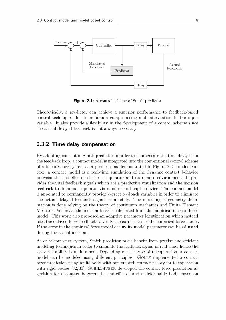
The Smith predictor, depicted in Figure 2.1 genuinely introduced by O.J.M. Smithin 1957. There are different implementations and the exact control scheme of Smithpredictor is not conclusive because of differences in individual control requirements.However, it is absolute that the method proposes a solution to time delay problemby allowing the controller to respond to the simulated feedback signal instead ofsolely to the actual feedback signal. A simulated or predicted feedback signal isobtained by the model of the actual process but without physical time delay. Anactual feedback signal can be generally required for the controller to response if theresidual error in the control loop remains. With this principle, the stability of theoverall control loop can be improved accordingly due to reduction in task completiontime [8,84,85], provided that the contact mechanics or the actual process is known.
2.3 Contact model and model based control 8
Controller Process
SimulatedFeedback
Delay
ActualFeedback
Predictor
Delay
Input
−−
++
Figure 2.1: A control scheme of Smith predictor
Theoretically, a predictor can achieve a superior performance to feedback-basedcontrol techniques due to minimum compromising and intervention to the inputvariable. It also provide a flexibility in the development of a control scheme sincethe actual delayed feedback is not always necessary.
2.3.2 Time delay compensation
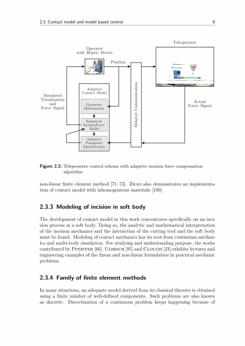
By adopting concept of Smith predictor in order to compensate the time delay fromthe feedback loop, a contact model is integrated into the conventional control schemeof a telepresence system as a predictor as demonstrated in Figure 2.2. In this con-text, a contact model is a real-time simulation of the dynamic contact behaviorbetween the end-effector of the teleoperator and its remote environment. It pro-vides the vital feedback signals which are a predictive visualization and the incisionfeedback to its human operator via monitor and haptic device. The contact modelis appointed to permanently provide correct feedback variables in order to eliminatethe actual delayed feedback signals completely. The modeling of geometry defor-mation is done relying on the theory of continuum mechanics and Finite ElementMethods. Whereas, the incision force is calculated from the empirical incision forcemodel. This work also proposed an adaptive parameter identification which insteaduses the delayed force feedback to verify the correctness of the empirical force model.If the error in the empirical force model occurs its model parameter can be adjustedduring the actual incision.
As of telepresence system, Smith predictor takes benefit from precise and efficientmodeling techniques in order to simulate the feedback signal in real-time, hence thesystem stability is maintained. Depending on the type of teleoperation, a contactmodel can be modeled using different principles. Golle implemented a contactforce prediction using multi-body with non-smooth contact theory for teleoperationwith rigid bodies [32, 33]. Schillhuber developed the contact force prediction al-gorithm for a contact between the end-effector and a deformable body based on
2.3 Contact model and model based control 9
Operatorwith Haptic Device
Teleoperator
Delayed Communication
SimulatedVisualization
andForce Signal
Position
GeometryDeformation
EmpiricalIncisionForce
Model
AdaptiveContact Model
ActualForce Signal
AdaptiveParameter
Identification
Figure 2.2: Telepresence control scheme with adaptive incision force compensationalgorithm
non-linear finite element method [71–73]. Zhao also demonstrates an implementa-tion of contact model with inhomogeneous materials [100].
2.3.3 Modeling of incision in soft body
The development of contact model in this work concentrates specifically on an inci-sion process in a soft body. Doing so, the analytic and mathematical interpretationof the incision mechanics and the interaction of the cutting tool and the soft bodymust be found. Modeling of contact mechanics has its root from continuum mechan-ics and multi-body simulation. For studying and understanding purpose, the workscontributed by Pfeiffer [66], Ulbrich [95] and Clough [23] exhibits lectures andengineering examples of the linear and non-linear formulation in practical mechanicproblems.
2.3.4 Family of finite element methods
In many situations, an adequate model derived from its classical theories is obtainedusing a finite number of well-defined components. Such problems are also knownas discrete. Discretization of a continuous problem keeps happening because of

2.3 Contact model and model based control 10
the presentation limitations of a complex behavior in one operation [102]. Fromclassical theories of mechanics to the actual implementation, the family of finiteelement methods keep repeating their success as an essential simulation of tool in thisvery computing age. The development of the finite element has become a principlewith scientific contributions in every way. As for engineers, the discretization ofcontinuous problems has been approached intuitively by creating an analogy betweenreal discrete elements and finite portions of a continuum domains. This statementis also true to the approaches discussed in this research work.
In the early time of developing the principle of finite element especially in the fieldof solid mechanics, McHenry [54] Hrenikoff [45] Newmark [60,61] and South-well [86] showed evidences that reasonably good solutions to an elastic continuumproblem can be obtained by replacing small portions of the continuum by an ar-rangement of simple elastic bars. Later, Tuner et al [94]. demonstrated a moredirect substitution of properties can be made effectively by considering small por-tions or elements in a continuum behaving in a simplified manner. One of the mostimportant contributions was given by Zienkiewicz and Taylor [101, 102] whogathered the necessary and relevant mathematical analysis into what would be calledthe Finite Element Method (FEM), building the pioneering mathematical formalismof the method. The books of Bathe [13], Wriggers [98, 99], Belytschko [15] andEberhard [26] are suitable for introductory but crucial examples to engineeringfinite element applications and problem formulations.
The first effort for developing the Extended Finite Element Method (XFEM) method-ology can be traced back to 1999 when Belytschko and Black presented aminimal remeshing Finite Element Method for crack growth [14]. They added dis-continuous enrichment functions to the Finite Element approximation to accountfor the presence of the crack. This method allows the crack to be arbitrarily alignedwithin the mesh. Moës later improved the method and called it the Extended FiniteElement Method [56,57]. A major contribution in this area can also be found in thedissertation of Dolbow [25]. XFEM has been adopted into number of problemsinvolving the discontinuities in the element while requires minimum considerationon the mesh condition [29]. The minimum consideration of mesh condition is knownas the main advantage of XFEM in contrast to FEM which generally requires recon-sideration of mesh when treated with discontinuity. The more recent and profoundworks in this field can also be referred to ones of Sukumar, Bordas, Hansbo andHansbo and Fries [16, 29, 39, 89]. Mohammadi has published an introduction toXFEM comprising a range of enrichment methods for different discontinuity typesin solid mechanics [58].
Both FEM and XFEM are popular as implementation tools of real-time interactivegeometry deformation simulations. Since the simulation of the deformation of suchcomplex bodies requires a discretization to be efficient. Both methods are alsosuitable to the computing and graphic visualization which demonstrates a full bodyas a finite number of elements or triangles. Terzopoulos exhibited a dynamicsimulation of a soft-body and the rendering of the contact force allowing interactionwith a haptic device [91]. Jeřábková demonstrates a use of XFEM and parallelized
2.3 Contact model and model based control 11
computing on a multi-cored CPU [46] to achieve a simulation of virtual cutting.Conti et al. invents an open-sourced haptic development library CHAI3D whichprovides a rapid haptic scene developing framework. Similarly, SOFA framework isdeveloped by Allard et al. combine FEM and XFEM functionality and intuitivehaptic interface. A possibility of an automatic performance evaluation of the surgicalsimulator was demonstrated by Sewell [75].
The computational expense of the simulation is another challenge preventing a suc-cessful realization of contact model or Smith predictor concept in a telepresencesystem. It is arguable that a contact model should not involve in an complicate con-tact due to its inefficiency to substitute the feedback variables with a task completiontime smaller than the actual time delay in the communication. This statement hasbeen true for a computational point of view. Nonetheless, a simulation of incisionespecially with a soft-body requires that level of complexity. However, with moderncomputational techniques and hardwares, a real-time simulation of contact phenom-ena with multi-level of optimization is in their progress and has been improveddramatically in the recent years. One major aspect which minimize the computa-tional time of such complex simulator is the modern computing architecture, bothsoftware and hardware such as parallel computing on multi-cored CPU and graphiccard [2, 3, 5].
3 Incision mechanics in a soft body
A first step in considering a physical model should be a clear and precise elaborationof the purpose of the kinematic model. The different approaches may lead to differentresults. In any case the chances of establishing a proper model depend strongly ona thorough understanding of the physical processes of the object to be modeled. Agood model can be referred as a good representation of mechanical properties andtherefore a good correspondence to practice and its measurement [66].
This chapter is the beginning of the main objective of this work, which is the devel-opment of a contact model for a medical incision process. For the visualization ofthe dynamic geometry deformation required by the contact model, a physical modelof incision mechanics must be investigated before the governing system of equationscan be derived. Doing so, the definition of an incision or a cut in a solid body on thebasis of continuum mechanics will be discussed in this chapter. Since the simulationof an incision in a large a solid body is the intention of this work, the derivationof kinematic variables and the governing system of equations using a linear strainmeasure is sufficient.
Some formulations found in this chapter are also known in fracture mechanics such asderivations of Belytschko, Black, Moës and Gürses [14, 36, 56, 57]. Althoughthey were genuinely developed to handle the fracture and crack growth simulation,their derivations treat cracks and cuts similarly as a strong material discontinuityin a solid body with also applicable for modeling of a cut in a solid body.
3.1 Definition of a cut in a solid body
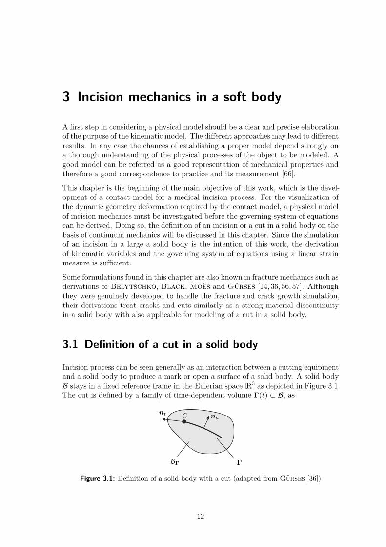
Incision process can be seen generally as an interaction between a cutting equipmentand a solid body to produce a mark or open a surface of a solid body. A solid bodyB stays in a fixed reference frame in the Eulerian space IR3 as depicted in Figure 3.1.The cut is defined by a family of time-dependent volume Γ(t) ⊂ B, as
BΓ Γ
nant C
Figure 3.1: Definition of a solid body with a cut (adapted from Gürses [36])
12
3.2 Kinematics 13
Γ(t1) ⊂ Γ(t2) for t1 ≤ t2 (3.1)
with a smooth boundary ∂Γ(t). In crack propagation, this boundary is often referredas the crack tip or front [36]. In a similar manner the definition of a cut says thatthe cut propagation is allowed only through the motion of the front ∂Γ. The currentcut volume is therefore derived as the set
Γ(t) = Γ(0) ∪
∂Γ(t) | 0 < t < t
(3.2)
where Γ(0) is the initial cut volume. In the current configuration at time t, particlesin body B occupy the region
BΓ(t) := B \ Γ(t) ∪ ∂Γ(t) ⊂ IR3 (3.3)
which have the outer boundary ∂B and the inner boundary formed by cut. Thetangential vector nt defies the direction of the cut Γ and points where the cut willevolve. The normal vector na, on the other hand, is perpendicular to the cut volume∂Γ. The rate of cut evolve shall be zero on the volume of the cut which is not thecut front C.
3.2 Kinematics
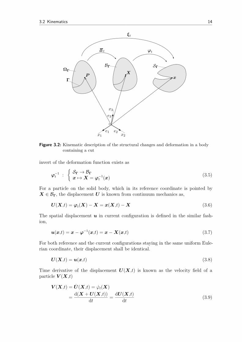
The structural changes and deformation occurs to the solid body B is depicted byFigure 3.2. The cut in general causes the structural changes in a solid body, whichis denoted by Γ on the domain ΩΓ. The same cut is then mapped as the geometrychanges to the solid body domain in reference coordinate known as BΓ. The geome-try changes due to cut including Dirichlet and Neumann boundary condition causethe deformation in the current configuration SΓ.
The coordinate vector X ∈ BΓ ∪ Γ(t) is referred to the material or Lagrangian
coordinates of a particle in a solid body B in its reference configuration. In adeformed or current configuration at time t, the same particle is denoted by thevector in spatial or Eulerian coordinate x(X,t) ∈ SΓ , where SΓ ⊂ IR3.
3.2.1 Deformation
The deformation ϕt can be mapped accordingly by
ϕt :
BΓ → SΓ
X 7→ x = ϕt(X)(3.4)
The deformation ϕt is therefore only valid for the particles in body B which are noton the cut and cut boundary X /∈ Γ ∪ ∂Γ at their reference configuration. The
3.2 Kinematics 14
0
x1
e1x2
e2
x3
e3
xX
P
ϕt
ξt
Ξt
BΓ
ΩΓ
Γ
SΓ
Figure 3.2: Kinematic description of the structural changes and deformation in a bodycontaining a cut
invert of the deformation function exists as
ϕ−1t :
SΓ → BΓ
x 7→X = ϕ−1t (x)
(3.5)
For a particle on the solid body, which in its reference coordinate is pointed byX ∈ BΓ, the displacement U is known from continuum mechanics as,
U (X,t) = ϕt(X)−X = x(X,t)−X (3.6)
The spatial displacement u in current configuration is defined in the similar fash-ion,
u(x,t) = x−ϕ−1(x,t) = x−X(x,t) (3.7)
For both reference and the current configurations staying in the same uniform Eule-rian coordinate, their displacement shall be identical.
U (X,t) = u(x,t) (3.8)
Time derivative of the displacement U (X,t) is known as the velocity field of aparticle V (X,t)
V (X,t) = U (X,t) = ϕt(X)
=d(X +U (X,t))
dt=
dU(X,t)
dt(3.9)

3.2 Kinematics 15
and for the spatial velocity field v(X,t)
v(X,t) = u(X,t) = V (X,t) (3.10)
The second time derivative of the displacement U (X,t) represents the accelerationfield of a particle A(X,t)
A(X,t) = V (X,t) = U(X,t)
=dV (X,t)
dt=
d2U (X,t)
dt2(3.11)
and the spatial of the acceleration field a(X,t)
a(X,t) =dv(x,t)
dt=∂v(x,t)
∂t+∂v(x,t)
∂x·v(X,t)
3.2.2 Material structural and spatial configurational changes
A one-to-one piecewise transformation Ξt : ΩΓ → BΓ of the reference configurationis introduced to map the material structural changes due to cut in the body B [36].This mapping is considered as the time-dependent parameterization of the mediumthat accounts for the material structural changes such as a cut evolution governedby the cut tip ∂Γ. It coincides with the time-dependent change from the referencecoordinates P ∈ ΩΓ to the Lagrangian coordinates X ∈ Γ ∪ ∂Γ.
Ξt :
ΩΓ → BΓ
P 7→X = Ξt(P )(3.12)
In addition, the spatial configurational change ξt is given to map the change occursin material and structure of the body B to the actual coordinate of a particle atcurrent time configuration x, as
ξt :
ΩΓ → SΓ
P 7→ x = ξt(P )(3.13)
3.2.3 Deformation gradient
In the domain BΓ := B\Γ(t) ∪ ∂Γ(t), where the cut is excluded, the measurementof the local deformation is given by deformation gradient,
F :=∇ϕt(X) =∂ϕt∂X
=∇x(X,t) =∂x
∂X(3.14)
Since F is the derivative of the current position x of a particle at time t with respectto the coordinates of the reference configurationX, it describes the relation between

3.2 Kinematics 16
a line segment in the reference configuration and the corresponding segment in thecurrent configuration. The deformation gradient can be interpreted as a measurefor the deformation of a line segment dX, with
dx = FdX (3.15)
Similarly, there are relations called transport theorems for the deformations of in-finitesimal surfaces
da = JF−T dA (3.16)
and volumes
dv = J dV (3.17)
The determinant of F recognized from the Nanson’s formula
J = detF (3.18)
is known as Jacobian and is used to measure the local change of volume.
3.2.4 Stress and strain
The Cauchy stress vector T is defined from a traction force vector∆f acting on aninfinitesimal area ∆A as
T = lim∆A→0
∆f
∆A(3.19)
With the surface normal vector n, the Cauchy stress vector is derived as
T = σ·n = σT ·n (3.20)
Tensor σ is called Cauchy stress tensor. To fulfill the spatial balance of angularmomentum, the Cauchy stress tensor is always symmetric and belongs to the currentconfiguration by definition. σij where i = j denotes the normal stress, whereasσij where i 6= j are shear stress. The stress tensor describes the state of stressin a solid body, hence it must be determined in terms of one of a configuration orcoordinate system.
The deformation gradient F is not a suitable measure of the actual deformation
of a material point due to its dependence on the motion of a solid body
(
∂x
∂X
)
.
The Green-Lagrange strain is introduced instead to eliminate this problem. TheGreen-Lagrange strain tensor is non-linear and often considered as a better measurecompared to the deformation gradient since it measures the strain by compare the
3.2 Kinematics 17
rate of displacement U in the reference configuration X as
EX =1
2
(
∇XuT +∇Xu+∇Xu
T ·∇Xu)
(3.21)
or index-wise
EXij =1
2
(
∂ui
∂Xj
+∂uj
∂Xi
+∂uk
∂Xi
∂uk
∂Xj
)
(3.22)
Obviously, the Green-Lagrange strain tensor is configuration dependent, thereforeEX 6= Ex. In context of this work, which is focusing on the modeling of incisionprocess, the deformation is considered to be small with respect to the total geometryof the test scenery. Thus for a small displacement in a solid-body ‖∆U‖, thereexists from linearization that a kinematic variable which is partial differentiatedwith respect to X is
∂ •
∂X=∂ •
∂x·∂x
∂X=∂ •
∂x·∂ (X +U)
∂X≈∂ •
∂x(3.23)
With this linearization, the Green-Lagrange strain tensor is simplified into the sym-metric infinitesimal strain tensor ǫ.
EXij ≈ Exij =1
2
(
∂ui
∂xj
+∂uj
∂xi
)
:= ǫij (3.24)
3.2.5 Constitutive equations
Previously, it was shown that the stresses in a solid body made of elastic materialis a result from the deformation of the material. The deformation is also possible toexpress them in terms of strain. To obtain it, the relation between the stress andstrain known as Hooke’s material law is brought in Equation 3.25.
σ = C : ǫ or σij = Cijklǫkl (3.25)
It is capable of providing a explanation of the linear elastic material behavior. The4th-order strain tensor C := C4 contains 34 = 81 independent elements Cijkl. How-ever, because of the symmetry of both the stress tensor σ and the strain tensor ǫ,the number of independent elements is reduced to 36. Together with the consid-eration of the strain energy of a linear elastic anisotropic material, the number isagain reduced to 21. For an orthotropic material, there are only nine independentelements to be considered. If the material is isotropic, the strain tensor C can becompletely determined by two independent elements, the Young’s modulus E andPoisson ration ν, or Lamé parameters λ and µ
σ = λtr(ǫ)I + 2µǫ or σij = λǫkkδij + 2µǫij (3.26)

3.3 Conservation of momentum 18
with
λ =νE
(1 + ν)(1− 2ν)and µ =
E
2(1 + ν)(3.27)
With equation 3.26, the stress tensor is recognized as
σ11 σ12 σ13
σ21 σ22 σ23
σ31 σ32 σ33
=
2µǫ11 + λ(ǫ11 + ǫ22 + ǫ33) 2µǫ12 2µǫ13
2µǫ21 2µǫ22 + λ(ǫ11 + ǫ22 + ǫ33) 2µǫ23
2µǫ31 2µǫ32 2µǫ33 + λ(ǫ11 + ǫ22 + ǫ33)
(3.28)
Thus, the determination of each element of tensor C can be concluded as
C1111 = C2222 = C3333 = 2µ+ λ
C1122 = C1133 = C2211 = C2233 = C3311 = C3322 = λ (3.29)
C1212 = C1313 = C2121 = C2323 = C3131 = C3232 = 2µ
The other elements of the tensorC are known to be zero. To simplify and also reduceunnecessary elements, the stress and strain tensor are often sorted in a vector-forminstead as
σ = [σ11 σ22 σ33 σ12 σ23 σ13] and ǫ = [ǫ11 ǫ22 ǫ33 2ǫ12 2ǫ23 2ǫ13] (3.30)
Using the tensors in vector-form, an extra caution must be taken since the conven-tional coordinate transformation may not valid. Take this into account, the stresstensor is known as,
σ = C · ǫ (3.31)
For isotropic material, the strain tensor C := C ∈ IR6x6 can be simplified as
C =E
(1 + ν)(1− 2ν)
1− ν ν νν 1− ν ν 0
ν ν 1− ν12− ν 0 0
s 0 0 12− ν 0
0 0 12− ν
(3.32)
For a further extensive discussion on Cauchy stress tensor, the interested reader isencouraged to consult [15,26,101,102] for the relation between material tensor formsand their matrix quantities.
3.3 Conservation of momentum
The law of conservation of mass states that mass of a closed system will remain con-stant over time, when the mass to energy conversion is not considered. Therefore,
3.4 Boundary value problems 19
the mass is conserved in reference and current configurations. ρ are the constantmaterial density of a solid body at both reference and current configurations respec-tively. Thus,
m(t) =∫
SΓ
ρ(x,t)dv =∫
BΓ
ρ(X)JdV (3.33)
The Newton’s second law of motion for a continuum or the momentum conservationprinciple in Equation 3.34 is collectively recognized as the strong form. It statesthat the material time derivative of the linear momentum equals the net force.
L(t) =∫
SΓ
ρ udv =∫
SΓ
ρ bdv +∫
∂SΓ
Tda (3.34)
Where ρb is body force per unit volume and T is known from Cauchy boundarystress vector acting on the surface ∂SΓ of a volume. Apply the Cauchy stress vectorknown from equation 3.20 to equation 3.34 provides
∫
SΓ
ρ udv =∫
SΓ
ρ bdv +∫
∂SΓ
σ·nda (3.35)
Employing the Grauß’s integral theorem, the equation 3.35 can be written as
∫
SΓ
ρ udv =∫
SΓ
ρ bdv +∫
SΓ
divσdv (3.36)
or∫
SΓ
(ρ b− ρ u+ divσ) dv = 0 (3.37)
Equation 3.37 must be valid for a whole body SΓ, therefore the integrand must equalzero. This assumption points to the local balance of momentum for any particle onthe body. Therefore, Equation 3.38 which is known as the governing system ofequations is obtained.
ρ (b− u) + divσ = 0 (3.38)
or index-wise,
ρ (bi − ui) +∂σi
∂xj
= 0 (3.39)
3.4 Boundary value problems
The purpose of applying boundary values to the governing system of equations is tosolve the equations with prescribed support displacements, tension forces and the

3.4 Boundary value problems 20
geometry alternation due to cut.
T 0
T
BΓ ∂Bϕ
∂Bt
Γ
SΓ∂Sϕ
∂St
U0
u
C
nt na
Figure 3.3: Boundary value problem of a solid body in reference BΓ and currentSΓconfigurations
The main challenge of modeling of an incision process lies by how the materialstructural changes are properly treated as the boundary conditions. To begin with,Figure 3.3 is referred. The same solid body B has the outer boundary values ∂Sin its current configuration of domain SΓ. ∂S are given by the all known boundaryconditions including where the cut area exists.
∂S = ∂Sϕ ∪ ∂St (3.40)
Analogously, both boundaries exhibits no intersection. Thus,
∂Sϕ ∩ ∂St = ∅ (3.41)
Prescribed displacements ∂Sϕ are known as Dirichtlet boundary conditions or es-sential boundary conditions. The prescribed displacements in current configurationare denoted by u
In contrast, prescribed loads ∂St on the surface of the solid body and the cut arereferred as Neumann boundary conditions or natural boundary conditions. They areassumed automatically on all remaining boundaries. The prescribed loads in currentconfiguration are given by the traction force vector T . In addition, the tractioncaused by the cutting tool to the solid body is described as part of prescribed loads.However, the inner boundary condition of both faces surrounding the cut Γ recallsno surface traction. Thus,
σ·na = T (x) = 0 where x ∈ ∂Γ (3.42)
3.5 Remapping of the governing system of equations 21
3.4.1 Initial value problems
The initial value problems considers all boundary conditions ∂B correspond to thestate of the solid body in its reference configuration B−. In technical mechanics,the initial state often correspond to the reference time t = 0. Since the incisionemploys the material structural changes Ξt and causes the changes in the referenceconfiguration, the context of reference is therefore confusing due to the referenceconfiguration is time-dependent according to the material structural changes [36].
Despite the extensive use of the classical definition of the initial boundary valuesin this work, they are defined in a different manner. The current configuration inthis work is clearly denoted by the configuration which the solid body occupies afterthe material structural changes. Their boundary values are given similarly to theones of the current configuration as ∂B = ∂Bϕ ∪ ∂Bt. The time-dependency of thereference configuration forces the boundary values to be remapped as discussed insection 3.5
The actual prescribed displacements and loads in reference configuration are requiredfor the governing system of equations to be solvable. Additionally, if the dynamicbehavior is as of interest, the displacement velocity must be given as well. Theinitial boundary value problems can be summarized as
U (X,t = 0) = U 0 (3.43)
U (X,t = 0) = U 0 (3.44)
T (X, t = 0) = T 0 and (3.45)
T (X, t = 0) = 0 where X ∈ Γ (3.46)
3.5 Remapping of the governing system ofequations
The governing system of equations 3.38 illustrates the dynamic deformation ofa solid body with respect to its current geometry, body force and the surfacetraction applied in its current configuration. On the other hand, domain BΓ :=B\Γ(t) ∪ ∂Γ(t) changes over time as the cut Γ(t) evolves. Depending on how thematerial structural changes Ξt occur – or in context of this work, the type of cut –the governing system of equations must be reconsidered as follow.
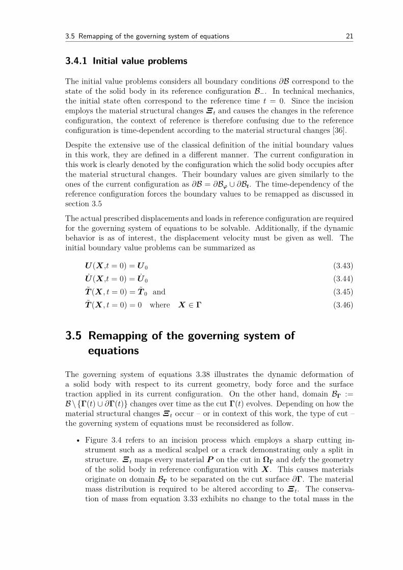
• Figure 3.4 refers to an incision process which employs a sharp cutting in-strument such as a medical scalpel or a crack demonstrating only a split instructure. Ξt maps every material P on the cut in ΩΓ and defy the geometryof the solid body in reference configuration with X. This causes materialsoriginate on domain BΓ to be separated on the cut surface ∂Γ. The materialmass distribution is required to be altered according to Ξt. The conserva-tion of mass from equation 3.33 exhibits no change to the total mass in the
3.6 Weak form of conservation of momentum 22
solid body and remain constant (m(t) = m0). The displacement u of currentconfiguration x can be obtained by solving the governing system of equations.
x1
x2
X1,2P
BΓΩΓ SΓ
C CC
Γ
Figure 3.4: Mapping change due to incision or split in structure
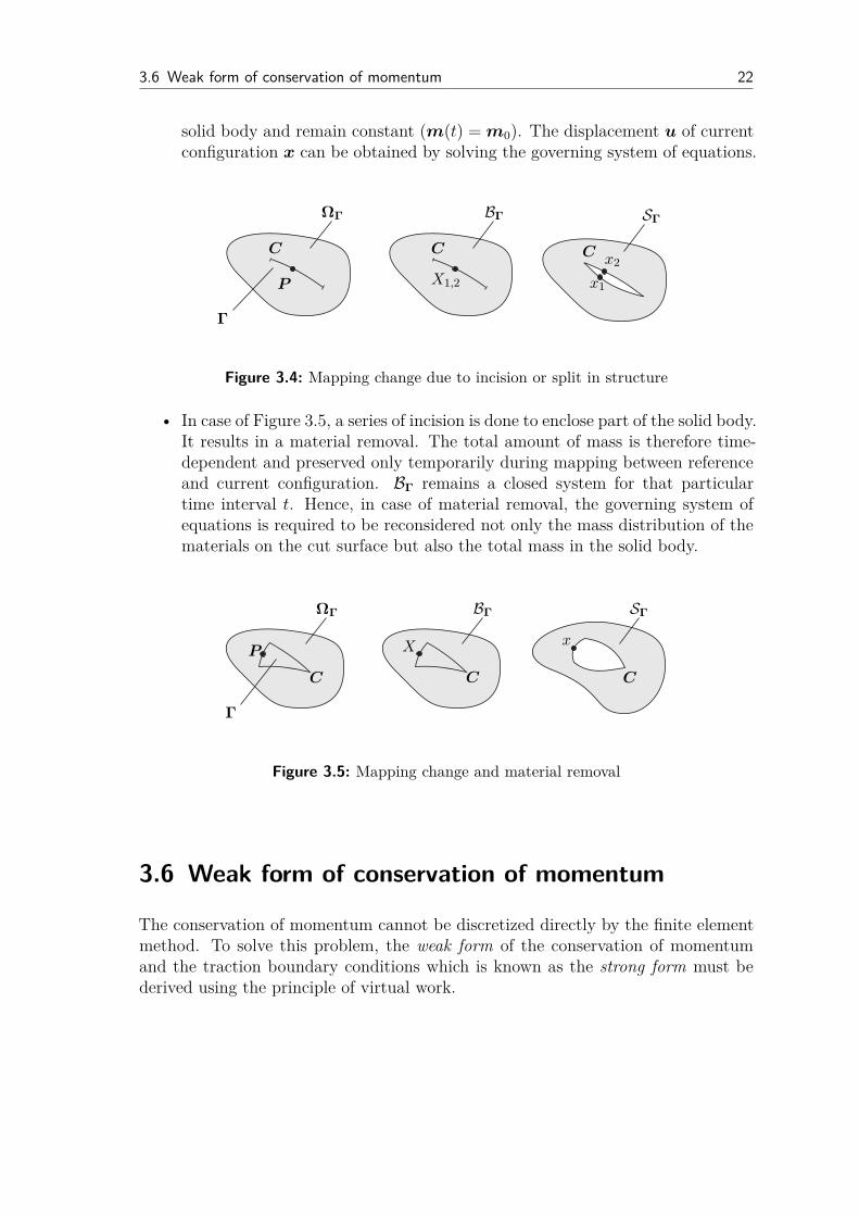
• In case of Figure 3.5, a series of incision is done to enclose part of the solid body.It results in a material removal. The total amount of mass is therefore time-dependent and preserved only temporarily during mapping between referenceand current configuration. BΓ remains a closed system for that particulartime interval t. Hence, in case of material removal, the governing system ofequations is required to be reconsidered not only the mass distribution of thematerials on the cut surface but also the total mass in the solid body.
xXP
BΓΩΓ
Γ
SΓ
CCC
Figure 3.5: Mapping change and material removal
3.6 Weak form of conservation of momentum
The conservation of momentum cannot be discretized directly by the finite elementmethod. To solve this problem, the weak form of the conservation of momentumand the traction boundary conditions which is known as the strong form must bederived using the principle of virtual work.
3.6 Weak form of conservation of momentum 23
3.6.1 Strong to weak form
A weak form will now be developed for the conservation of momentum introducedin Equation 3.34 and the traction boundary conditions mentioned in the section 3.4.For this purpose, the trial function u(X,t) is employed to satisfy all displacementboundary conditions and to be smooth enough so that all derivatives in the conserva-tion of momentum equation are well defined. The test function δu(X) are assumedto be smooth enough so that all of the following steps are well defined and to vanishon the prescribed displacement boundary.
The weak form is obtained by taking the product of the conservation of momentumequation with the test function and integrating over the domain [15]. The integralof this product must be zero. For that in the reference configuration,
∫
BΓ
[ρ(b− u) +∇xσ] δu dV = 0 (3.47)
or with equation 3.39, the equation above can be written index-wise as
∫
BΓ
[
ρ(bi − ui) +∂σik
∂xk
]
δujdV = 0 (3.48)
with the product rule known as
∂a(x)
∂xb(x) =
∂(a(x)b(x))
∂x− a(x)
∂b(x)
∂x(3.49)
By-part integration of the stress term by employing the Grauß’s integral theoremyields
−∫
BΓ
∂δuj
∂xk
σijdV +∫
BΓ
∂(δujσik)
∂xk
dV +∫
BΓ
ρ(bi − ui)δujdV = 0 (3.50)
Using the divergence theorem, the surface traction is derived as
∫
BΓ
∂(δujσik)
∂xk
dV =∫
∂BΓ
δujσiknkdA =∫
∂BΓ
δujTidA (3.51)
Substitution of this surface traction in equation 3.50 provides
−∫
BΓ
∂δuj
∂xk
σikdV +∫
∂BΓ
δujTidA+∫
BΓ
(δujbi − δujρui)dV = 0 (3.52)
The term∫
∂BΓ
δujTidA are applied to all initial Dirichlet boundary conditions or the
essential boundary conditions known from section 3.4 as T 0(X). Thus the weak-
3.6 Weak form of conservation of momentum 24
form of the governing system of equation is
∫
BΓ
δujρbidV −∫
∂BΓ
δujT0dA+∫
BΓ
∂δuj
∂xk
σikdV +∫
BΓ
δujρuidV = 0 (3.53)
or
∫
BΓ
δuρbdV −∫
∂BΓ
δuT 0dA+∫
BΓ
∂δu
∂xσdV +
∫
BΓ
δuρudV = 0 (3.54)
3.6.2 Smoothness of the test function and the trial function
In classical derivations of the weak form, all functions appeared in the strong form areassumed to be continuous. For the conservation of momentum from equation 3.38to be well defined in a classical sense, the product of the nominal stress and theinitial area must be continuously differentiable, i.e. C1. Otherwise the first deriva-tive would exhibits discontinuities [15]. The trial function δu needs to satisfy alldisplacement boundary conditions. These conditions on the trial displacement areindicated symbolically by
u(X,t) ∈ U (3.55)
where U =
u(X,t) | u(X,t) ∈ 0C(X),u = U 0 on ∂Bϕ
Displacement fields which satisfy the condition pointed by equation 3.55, such asthe displacement fields which are in U , are called kinematically admissible. The testfunction δu is not time-dependent. Moreover, the test function is required to be C0
and to vanish on displacement boundaries, such as
δu(X,t) ∈ U0 (3.56)
where U0 =
δu(X,t) | u(X,t) ∈ C0(X), δu = 0 on ∂Bϕ
The prefix δ is denoted for all variables which are test functions and for variableswhich are functions of the test functions.
3.6.3 Principle of virtual work
For the purpose of obtaining a methodical procedure for developing the finite elementequations, the virtual works will be defined according to the type of work theyrepresent. Each of the terms in the weak form represent the work occurred due tothe test function δu, which is often called the virtual displacement to indicate thatit is actually the virtual and not an actual displacement. The principle of virtualwork says
δW (δu,u) ≡ δW int − δW ext + δW kin = 0 (3.57)
3.6 Weak form of conservation of momentum 25
The virtual work of the body force and the traction corresponds to the first andsecond terms in Equation 3.54 is called the virtual external work since it is theresult of the external loads and given by
δW ext =∫
BΓ
δuρbdV −∫
∂BΓ
δuT 0dA (3.58)
The third term of Equation 3.54 reflects the virtual internal work as a consequenceof the stresses in the material
δW int =∫
BΓ
∂δu
∂xσdV (3.59)
while the last term can be considered as a body force which acts in their directionopposite to the acceleration, i.e. a d’Alembert force. In context of this work, theterm is recognized as the virtual kinetic works, thus
δW kin =∫
BΓ
δuρudV (3.60)
The benefit of the virtual work in this viewpoint is to obtain the weak form forfurther discretization in the finite element approximation. Thus, the steps frommultiplying the equation with the test function and performing various manipula-tions can actually be avoided. The virtual work scheme is useful for memorizing theweak form due to its representativeness to the actual physical property of a closedsystem [15]. From mathematical perspective, the test function δu is not requiredto be a virtual displacements. It is allowed to be any test function which satisfiescontinuity conditions and vanish on the displacement boundaries as described byequation 3.56.

4 Finite element approach
The Finite Element Method or FEM is well known for its suitability and scalability ofmodeling a deformable body. FEM gains a major popularity in the real-time hapticand surgical simulation. It is also a suitable tool to discrete the governing system ofequations obtained from chapter 3 for contact model implementation. Using FEMA similar approaches can be seen in the works of demonstrating different types ofcontact mechanics for a telepresence application [71,100].
Both analysts and developers of FEM-based simulation should understand the fun-damental concepts of finite element analysis thoroughly. Without an understandingof the implication and meaning of the physical interpretation, FEM approximationmay be not be usable. Therefore, this chapter is devoted to an extensive discus-sion on the discretization of the weak form of the governing system of equationsobtained in section 3 and how the spatial discretization of FEM principle can beapplied to an individual material volume or element. This section will also addressesthe remapping problem between configurations which occurs due to a rapid changein the geometry of a soft body when an incision process is carried out.
4.1 Spatial discretization
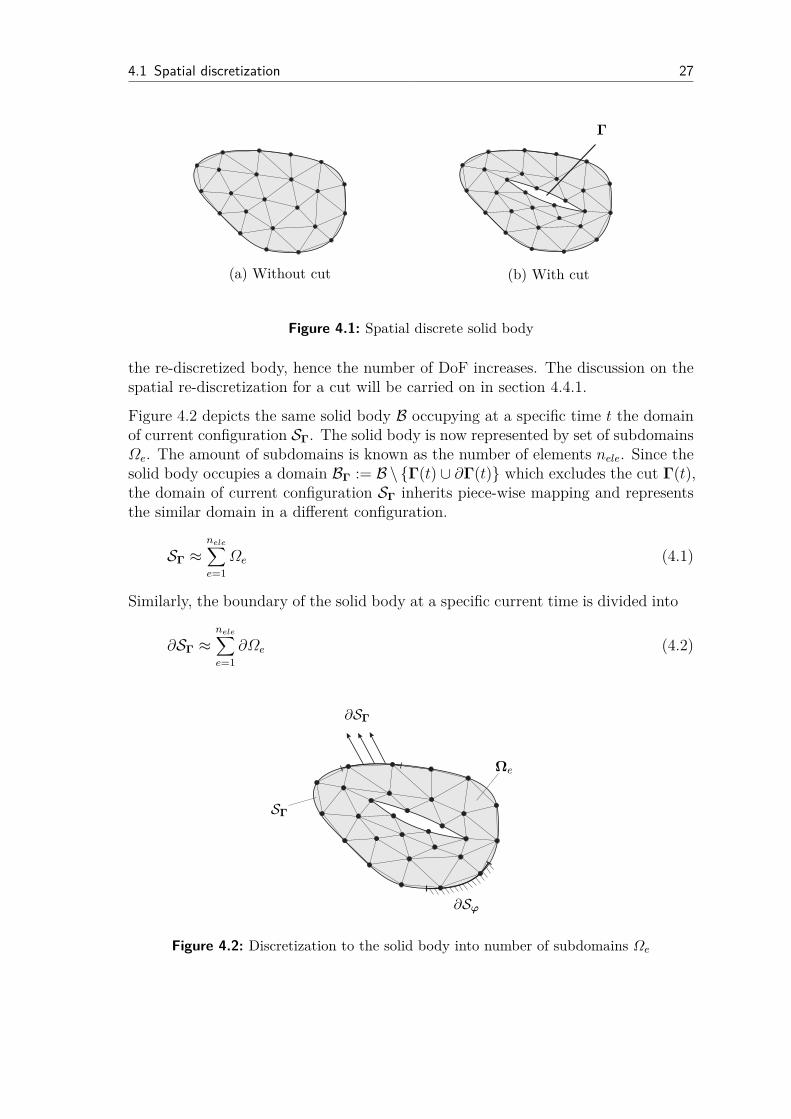
The approximation using finite elements begins with the spatial discretization of aproblem domain into finite numbers of units or elements. For a Lagrangian mesh,each element processes nodes mapped to fixed material points or particles. Thearrangement of the elements is called the topology indexing of nodal degree-of-freedoms (DoFs) in the governing system of equations. Thus, an element can beidentified by the index of the DoFs it uniquely occupies. In Figure 4.1(a) the solidbody B is discretized without exhibiting of a cut. The discrete body is a representa-tive of the considered deformation problem governing by the system of equations 3.38and 3.54. Figure 4.1(b) depicts the same solid body B with a cut, the elementsin the discrete representative body are arranged so that the elements match thegeometry of the cut. Both Figures demonstrate that the representative bodies donot match the actual domains neither with or without a cut exactly. Thus, theaccuracy of the approximation obtained from the model depends strongly on how asolid body is discretized since the beginning.
Also, if the solid body initially processed no cut in its body, a re-discretization isnecessary so that the geometry of the cut is presented properly. The topology isupdated so that the discrete body still represents the actual body geometry. Dependon the cut, the topology change may increase the number of elements required in
26
4.1 Spatial discretization 27
Γ
(a) Without cut (b) With cut
Figure 4.1: Spatial discrete solid body
the re-discretized body, hence the number of DoF increases. The discussion on thespatial re-discretization for a cut will be carried on in section 4.4.1.
Figure 4.2 depicts the same solid body B occupying at a specific time t the domainof current configuration SΓ. The solid body is now represented by set of subdomainsΩe. The amount of subdomains is known as the number of elements nele. Since thesolid body occupies a domain BΓ := B \ Γ(t) ∪ ∂Γ(t) which excludes the cut Γ(t),the domain of current configuration SΓ inherits piece-wise mapping and representsthe similar domain in a different configuration.
SΓ ≈nele∑
e=1
Ωe (4.1)
Similarly, the boundary of the solid body at a specific current time is divided into
∂SΓ ≈nele∑
e=1
∂Ωe (4.2)
Ωe
SΓ
∂Sϕ
∂SΓ
Figure 4.2: Discretization to the solid body into number of subdomains Ωe
4.2 Discrete governing system of equations 28
4.2 Discrete governing system of equations
The discrete equations for a finite element model are obtained from the principleof virtual work by using finite element interpolation for the test and trial functions.It employs the approximated solution on the nodes of each element to describe themotion of a solid body. The discretization is established in the initial configurationBΓ using isoparametric elements to interpolate the initial geometry in terms of theparticle denoted by Xj which defining the initial position of nodes in an elementas
X ≈n∑
j=1
Nj(X)Xj (4.3)
where Nj(X) are a shape function and n denotes the number of nodes per element.The shape function is be chosen to comply with the Kronecker Delta property
Nj(Xi) := δij =
0; i 6= j1; i = j
(4.4)
and the Partition of Unity
n∑
j=1
Nj(X) = 1 (4.5)
As for a Lagrangian mesh, during the motion, nodes and elements are permanentlyattached to the particles with which they were initially associated. Accordingly, thesubsequent motion can be described in terms of the current configuration xj(X,t)of a nodal particle.
x =n∑
j=1
Nj(X)xj (4.6)
In consistent with their kinematic derived in equation 3.7, the displacement u isinterpolated as
u =n∑
j=1
Nj(X)uj (4.7)
The test function known as virtual displacement δu is required to satisfy the linearindependence which is necessary to solve the discrete governing system of equations.The shape functions are also used for the test function δu in the weak form
δu =n∑
j=1
Nj(X)δuj (4.8)

4.2 Discrete governing system of equations 29
Analogously, the nodal displacement velocity and acceleration fields are obtainedas
u =n∑
j=1
Nj(X)uj and u =n∑
j=1
Nj(X)uj (4.9)
For a three-dimensional configuration, the shape function can be arranged in amatrix as
N =
N1 0 0 · · · Nn 0 00 N1 0 · · · 0 Nn 00 0 N1 · · · 0 0 Nn
(4.10)
The weak form of conservation of momentum derived in equation 3.54 was obtainedto associate with the discretization of the FEM. From Equation 3.24 and 4.7, theinfinitesimal strain tensor is approximated as
ǫij =1
2
(
∂ui
∂xj
+∂uj
∂xi
)
=1
2
(
∂Nikuk
∂xj
+∂Njkuk
∂xi
)
(4.11)
=1
2
(
∂Nik
∂xj
+∂Njk
∂xi
)
uk
The strain-displacement matrix B ∈ IR6×3n
ǫ = B·u (4.12)
with
B =
∂N1
∂x1
0 0 · · · ∂Nn
∂x1
0 0
0 ∂N1
∂x2
0 · · · 0 ∂Nn
∂x2
0
0 0 ∂N1
∂x3
· · · 0 0 ∂Nn
∂x3
∂N1
∂x2
∂N1
∂x1
0 · · · ∂Nn
∂x2
∂Nn
∂x1
0
0 ∂N1
∂x3
∂N1
∂x2
· · · 0 ∂Nn
∂x3
∂Nn
∂x2
∂N1
∂x3
0 ∂N1
∂x1
· · · ∂Nn
∂x3
0 ∂Nn
∂x1
(4.13)
is introduced.From Equation 3.32, substituting the strain tensor ǫ in the equa-tion 4.12 yields,
σ = C · ǫ = C ·B·u (4.14)
The weak form from Equation 3.54 is applied to an element Ωe with the discretizedu and the shape function to obtain
∫
Ωe
NTρbdV −∫
∂Ωe
NT T 0dA+∫
Ωe
BT CBdV u+∫
Ωe
NTρNdV u
δu = 0
(4.15)

4.3 Element coordinates 30
which introduces the following physical terms of an element
k(e) =∫
Ωe
BT CBdV ∈IR3n×3n Stiffness matrix (4.16)
m(e) =∫
Ωe
NTρNdV ∈IR3n×3n Mass matrix (4.17)
f(e)Ω
=∫
Ωe
NTρbdV ∈IR3n Body volume force vector (4.18)
f(e)∂Ω
=∫
∂Ωe
NT T 0dA ∈IR3n Surface traction vector (4.19)
The element damping matrix is a material property required for the dynamic simu-lation of a soft body in this work. It may be possible for the global damping matrixto be found by considering the total energy lost of the whole solid body [13] but notfor an element. Nevertheless, the calculated global damping matrix may be depen-dent to eigenfrequency of the solid body. Therefore, a decoupling element dampingsimilar to element mass and stiffness matrices can not be obtained. Because ofthis complexity of damping modeling, a common type of damping called Rayleighdamping is often employed in the linear and nonlinear incremental analysis of struc-tures [12,92]. Rayleigh damping assumes that the damping matrix is decoupled andproportional to the mass and stiffness matrices in the form of
d(e) = a m(e) + b k(e) ∈ IR3n×3n Damping matrix (4.20)
The coefficients a and b are selectable to obtain a desire damping value. UsingRayleigh damping yields another benefit necessary for vibration analysis. This im-plementation also allows the damping to be increased as the eigenfrequency increaseswhen a stiffer material is employed [23]. In this work, this approach is also adopted.The discrete dynamic governing equation for an element Ωe is therefore obtained inthe following form.
k(e) ·u+ d(e) · u = f(e)Ω
+ f(e)∂Ω−m(e) · u (4.21)
4.3 Element coordinates
FEM is usually developed with shape functions expressed in terms of parent elementcoordinates, often called element coordinates for brevity. The element coordinatescan be considered an alternative set of material coordinates in a well-adopted La-grangian mesh. Therefore, the shape functions in terms of element coordinates isintrinsically equivalent to expressing a term in material coordinates. The shape ofthe parent domain depends on the shape and the dimension of the element used todiscrete a solid body. The element coordinate is denoted by ζ in tensor notation.The map X = x(ζ,0) corresponds to the reference or initial configuration, while

4.3 Element coordinates 31
x = x(ζ,t) refers to the current configuration which is time-dependent. Thus, thereis valid a chain rule describing the shape functions in element coordinate as
∂Ni
∂x=∂Ni
∂ζ·∂ζ
∂x=∂Ni
∂ζ·J−1 or
∂Ni
∂xj
=∂Ni
∂ζk
∂ζk
∂xj
=∂Ni
∂ζk
[
J−1]
kj(4.22)
Because the determinant of the Jacobian refers to the volume change of an elementwith respect to the element coordinate, det(J) > 0. If det(J) ≤ 0 at any time, itmeans that the material density ρ ≤ 0, which is physically impossible [15]. Therefore,the Jacobian must be invertible.
In this work, solid bodies are all discretized using tetrahedral elements. As depictedin Figure 4.3, a tetrahedral element occupies a three-dimensional space with 4 nodesand has 12 degrees of freedom in total. It has 4 shape functions, which are N1 = ζ1,N2 = ζ2, N3 = ζ3 and N4 = 1− ζ1 − ζ2 − ζ3.
ζ1 ζ2
ζ3
1 1
1
Figure 4.3: A tetrahedral element
For a linear Finite Element approximation, the derivative of the shape function withrespect to the element coordinate is constant as follow
∂N
∂ζ=
1 0 00 1 00 0 1−1 −1 −1
(4.23)
With these properties, the strain-displacement matrix B from equation 4.12 can bewritten in element coordinate as well as the integrand BCB. Hence, the elementstiffness k(e) can be written in element coordinate specific for tetrahedral elementas
k(e) =∫
Ωe
BT CBdV =
1∫
0
1−ζ3∫
0
1−ζ2−ζ3∫
0
BT CBdetJ dζ1dζ2dζ3 (4.24)

4.4 Assembly and remeshing 32
In a similar manner, the element mass matrix m(e) in equation 4.17 is found as
m(e) =∫
Ωe
NTρNdV =
1∫
0
1−ζ3∫
0
1−ζ2−ζ3∫
0
NTρNdetJ dζ1dζ2dζ3 (4.25)
4.4 Assembly and remeshing
4.4.1 Assembly process
In Lagrangian mesh, the nodes and elements move with the material. Boundariesand interfaces coincide with element edges, so that their treatment is simplified.Quadrature points also move with the material, thus constitutive equations arealways evaluated at the same material points, which is advantageous for history-dependent materials and boundary conditions [15].
Each discrete element represents a certain amount of material in the solid bodywhich is decided during the discretization. As discussed in section 4.1, an elementoccupies a set of individual nodes called topology. The elements whose at leastone node share the same index of DoF are neighbor in Lagrangian mesh. Theseelement are coupled with each other. The assembly process is referred here by theunification operator
⋃
. It sorts a variable of neighbor elements together using theirunique indexes. Hence, nodal mass of each element can be assembled to together toprovide a global mass matrix
M =nele⋃
e=1
m(e) (4.26)
the global stiffness matrix
K =nele⋃
e=1
k(e) (4.27)
and the global damping matrix
D =nele⋃
e=1
d(e) (4.28)
The global element body force and the global surface traction force can also assem-bled together as
F ext =nele⋃
e=1
f(e)∂Ω
+nele⋃
e=1
f(e)Ω
(4.29)
As result, a discrete global dynamic system of equations is obtained in Equation 4.30

4.4 Assembly and remeshing 33
with the global nodal displacement denoted by the vector U .
F ext = MU +DU +KU (4.30)
4.4.2 Remeshing
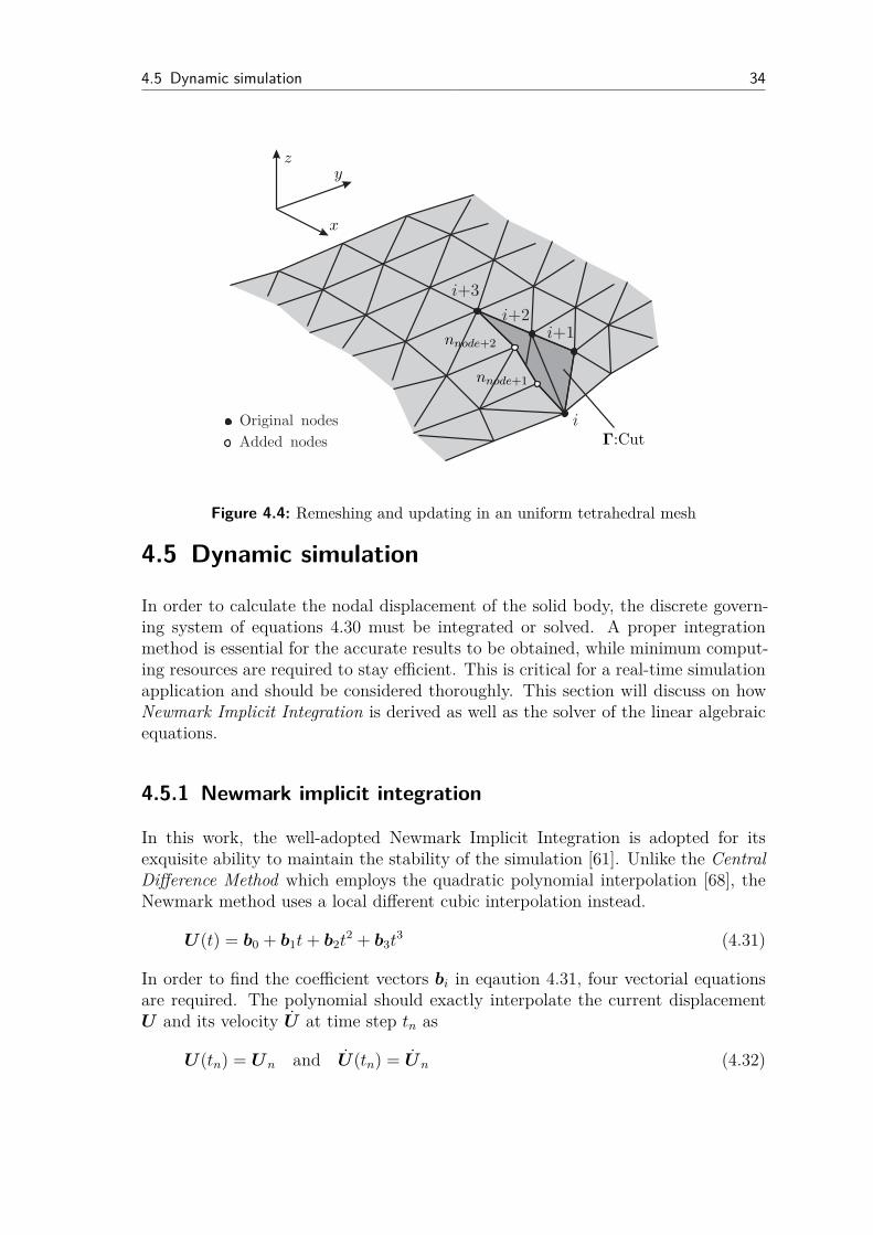
As mentioned earlier, Lagrangian meshes let the nodes and elements attached per-manently to the material points. The discussion in section 3.5 is the necessity ofremapping Ξt : ΩΓ → BΓ to preserve the validity of the governing system of equa-tions. For an incision simulation which the process contains a constant evolve ofa material discontinuity in a solid body, the remeshing process is compulsory forthe mesh to reasonably correspond to the actual geometry. In general, remeshingprocesses repeats the spatial discretization to a solid body into, so that the presentgeometry of the solid body is adequately represented.
The remeshing algorithm in this work is done by allowing the simulated object tobe cut in a vertical plane. Additionally, the scalpel is appointed to pass through aseries of nodes connecting a set of tetrahedral elements, as shown in Figure 4.4. Theemployed algorithm is required to demonstrate the increasing of the DoFs aroundthe opened surface. This methodology can be realized because the simulated objectis discretized so that the tetrahedral elements are uniformly arranged. A node ispointed by a unique index number which is one of local properties of a tetrahedralelement. To repeat the use of the same node number with no additional argumentcan be implied that two or more elements are occupying the same node and the cutdoes not exist between them. For this reason, the original nodes shall be multipliedby new additional nodes. Hence the total DoFs of the solid body will be generallyincreased due to the expansion of the surface.
Neumann and Dirichlet boundary conditions from the original mesh can be furtheradopted without any alternation, if the cut does not occur on the area where theNeumann and Dirichlet boundary conditions are constantly applied during the sim-ulation.
A remeshing process is required to be initiated each time the geometry change isexhibited. The change of DoF can be implied mathematically that the topologyof the governing system of equations 3.38 is not preserved and the actual solidbody is not identical to the original ones. Therefore, the assembly process mustbe called right after the remeshing process to reassembly a new governing systemof equations. There are remeshing techniques developed and optimized for eachsimulation problem. Interesting algorithms can be found in FEM-remeshing forcrack growth of Tradegard [93] and the tissue resection using delayed updates ina tetrahedral mesh shown done by Kundu in [49].
4.5 Dynamic simulation 34
+1i
+3i
+2i
Original nodes
Added nodes
i
nnode+1
nnode+2
x
yz
Γ:Cut
Figure 4.4: Remeshing and updating in an uniform tetrahedral mesh
4.5 Dynamic simulation
In order to calculate the nodal displacement of the solid body, the discrete govern-ing system of equations 4.30 must be integrated or solved. A proper integrationmethod is essential for the accurate results to be obtained, while minimum comput-ing resources are required to stay efficient. This is critical for a real-time simulationapplication and should be considered thoroughly. This section will discuss on howNewmark Implicit Integration is derived as well as the solver of the linear algebraicequations.
4.5.1 Newmark implicit integration
In this work, the well-adopted Newmark Implicit Integration is adopted for itsexquisite ability to maintain the stability of the simulation [61]. Unlike the Central
Difference Method which employs the quadratic polynomial interpolation [68], theNewmark method uses a local different cubic interpolation instead.
U (t) = b0 + b1t+ b2t2 + b3t
3 (4.31)
In order to find the coefficient vectors bi in eqaution 4.31, four vectorial equationsare required. The polynomial should exactly interpolate the current displacementU and its velocity U at time step tn as
U (tn) = Un and U (tn) = Un (4.32)

4.5 Dynamic simulation 35
Therefore, equation 4.31 is written in explicit form as
U (t) = Un + Un(t− tn) + b2(t− tn)2 + b3(t− tn)3 (4.33)
To determine the unknown displacement and its velocity at time tn+1 = tn+∆tn, thefollowing approaches are adopted from Burnett [20] by interpolate the displacementof time step tn+1
U (tn+1) = Un+1 = Un + Un∆tn1
2
(
(1− 2β) Un + 2βUn+1
)
∆t2n (4.34)
U (tn+1) = Un+1 = Un +(
(1− γ) Un + γUn+1
)
∆tn (4.35)
However, displacements and their velocities in both equations can not be calculatedbecause the acceleration Un+1 is still unknown. The following step of formulationemploys an implicit method which requires the information just only to the time ofconsideration. Thus, the acceleration from equation 4.34 is found as
Un+1 =Un+1 −Un − Un∆tn
β∆t2n−
(
1
2β− 1
)
Un (4.36)
This equation can be put into velocity in equation 4.35 to obtain
Un+1 = Un + (1− γ)∆tnUn + γ∆tnUn+1
= Un + (1− γ)∆tnUn+
γ∆tn
(
Un+1 −Un − Un∆tnβ∆t2n
−
(
1
2β− 1
)
Un
)
(4.37)
Substitute the acceleration in 4.36 and velocity in 4.37 in the linear dynamic gov-erning system of equations 4.30 at time tn+1 and obtain
MUn+1 +DUn+1 +KUn+1 = F extn+1 (4.38)
which is known in a recursive form as
K∗
nUn+1 = F extn+1 + F int
n (4.39)
with
K∗
n =
[
1
β∆t2nM +
γ
β∆tnD +K
]
(4.40)
F intn =
[
1
β∆t2nM +
γ
β∆tnD
]
Un +
[
1
β∆tnM +
(
γ
β− 1
)
D
]
Un+
[(
1
2β− 1
)
M +
(
γ
2β− 1
)
∆tnD
]
Un (4.41)
Using Newmark method exhibits the use of parameters β and γ, which stay in therange of 0 < β ≤ 0.5 and 0 ≤ γ ≤ 1. To choose proper values of these parameters,

4.5 Dynamic simulation 36
the following consideration must be made
• In general the Newmark integration by a linear system remains stable uncon-ditionally for γ ≥ 0.5 and β ≥ (γ + 0.5)2/4.
• For γ = 2β, the cubic interpolation will be comparable to the quadratic inter-polation and results in a constant acceleration.
• For β = 0.25 and γ = 0.5, the integration maintains unconditionally stable.This choice satisfies the trapezoidal rule which is also known as average accel-eration method. It was primary values proposed by Newmark. These valuesare majority in most of applications.
• With β = 1/6 and γ = 0.5, the method is comparable to linear accelerationmethods and is only conditionally stable depending on the system.
• If β = 0 and γ = 0.5, Newmark integration is identical to the Central Differ-ence method. This choice of parameters leads to a problem that the simulationtime step is governed by Courant stability limit. This limit can be interpretedthat the time-step must be small enough to capture the wave traveling throughan element which is equivalent to solving an oscillation at eigenfrequency ofthat element [37].
• At γ = 0.5, the method exhibits no additional damping rather than the naturalone found in the system equations. The higher value of γ will demonstratelarger numerical damping in the system.
Commonly, the explicit integration provides higher accuracy of the solution than theimplicit ones [52]. However, it requires the time-step ∆t to be very small in order topreserve the level of stability and solution accuracy. There is no ideal suggestion forwhich method is superior to the other. It depends strongly to the application andthe computing resources. In this work, the Newmark Implicit Integration methodis employed while choosing β = 0.25 and γ = 0.5 as stated in the general guide-lineabove. With Newmark method, the simulation is allowed to be adjusted so that thesize of time-step justify the computing resource while still provide the reasonablesampling rate of the simulation. However, time-step must be set to be small enoughto capture the oscillation of an interested mode of the simulation. In this work, thesimulation is appointed to serve as a visualization of the remote environment onthe monitor. For a small continuous deformation to average human eyes, a dynamicsimulation with sampling rate of 30Hz is sufficient which is equivalent to simulationtime-step of ≈ 0.033 s.
4.5.2 Solution of linear algebraic equations
The last section discussed exclusively on Newmark Implicit Integration which for-mulates the linear dynamic governing system of equations 4.30 in a familiar set oflinear algebraic equations. The displacement for the next simulation step is exhib-ited in equation 4.39 as vector Un+1. In order to solve the equation, equation 4.39
4.6 Implementation 37
will be partitioned and rearranged after given boundary condition of each DoF andtopology, also called index, as such
[
K∗
ϕ ϕ K∗
ϕ t
K∗
t ϕ K∗
t t
]
n
·
[
Uϕ
U t
]
n+1
=
[
F ϕ
F t
]ext
n+1
+
[
F ϕ
F t
]int
n
(4.42)
with nodal displacements Uϕ,n+1 are known from Dirichlet boundary conditions.F extt,n+1 are given nodal external forces which are identical to Neumann boundary
conditions. The solution of the rest nodal displacement in this linear algebraicequations for the next simulation step n+ 1 can then be written as
U t,n+1 = K∗−1t t,n
(
F extt,n+1 + F int
t,n −K∗
t ϕ,n ·Uϕ,n+1
)
(4.43)
After calculation of the nodal displacement Un+1, its velocity and acceleration canbe computed using equations 4.37 and 4.36 to obtain Un+1 and Un+1 for the nextsimulation step. The computation of the internal nodal forces from the elementcircling the node F int
n at current simulation step can be made with the completeregistration of Un, Un and Un. With earlier computation, the external nodal forcesF extϕ,n+1 of the next simulation step can be computed as
F extϕ,n+1 = K∗
t ϕ,n ·Uϕ,n+1 +K∗
t t,n ·Uϕ,n+1 − Fintϕ,n (4.44)
Equation 4.44 is not necessary to be computed in this work since it provides thereaction force of corresponding to given nodal displacements of the same indexes.The nodal external forces obtained from the FEM contains part of the incisionforce. They only reflect the external force causing a dynamic deformation in the softbody. To obtain the actual incision force, an empirical force model is purposefullyimplemented which will be extensively discussed later in chapter 7.
4.6 Implementation
Primarily, a simulation problem must be formulated. Algorithm 1 demonstrates theinitialization of a FEM simulation. The parameters, Young’s modulus E, densityρ and Poisson ratio ν must be given. They are essential for determination of thematerial type of the considered solid body. The mesh generation is employed to spa-tially discrete the continuum domain of the considered soft body into finite numberof tetrahedron elements at the current configuration BΓ of the beginning simulationtime tn = 0. The topology is also obtained determining a successive index of nodalDoFs. The initial Neumann and Dirichlet boundary conditions must be given. Usingthe topology index, element mass, damping and stiffness matrices will be calculatedand assembled to obtain the global system matrices. The formulation of the gov-erning system of equations is done so that the Newmark implicit integration can beemployed.
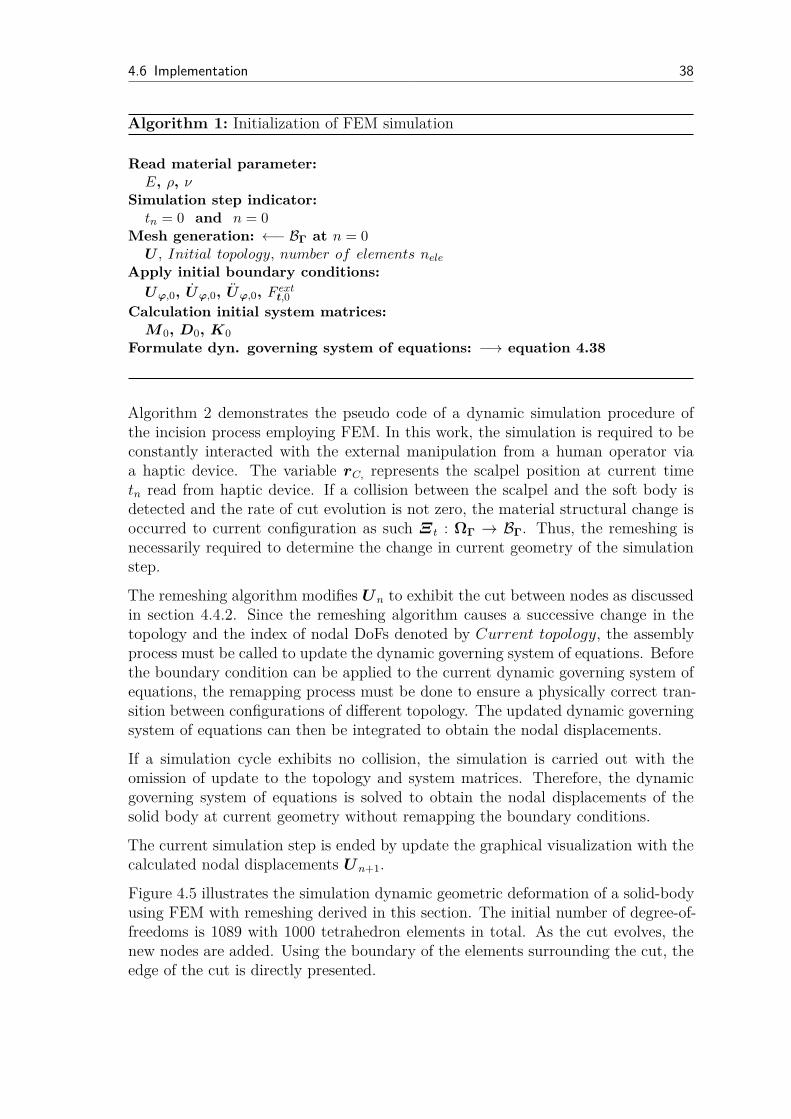
4.6 Implementation 38
Algorithm 1: Initialization of FEM simulation
Read material parameter:
E, ρ, νSimulation step indicator:
tn = 0 and n = 0Mesh generation: ←− BΓ at n = 0U , Initial topology, number of elements nele
Apply initial boundary conditions:
Uϕ,0, Uϕ,0, Uϕ,0, F extt,0
Calculation initial system matrices:
M0, D0, K0
Formulate dyn. governing system of equations: −→ equation 4.38
Algorithm 2 demonstrates the pseudo code of a dynamic simulation procedure ofthe incision process employing FEM. In this work, the simulation is required to beconstantly interacted with the external manipulation from a human operator viaa haptic device. The variable rC, represents the scalpel position at current timetn read from haptic device. If a collision between the scalpel and the soft body isdetected and the rate of cut evolution is not zero, the material structural change isoccurred to current configuration as such Ξt : ΩΓ → BΓ. Thus, the remeshing isnecessarily required to determine the change in current geometry of the simulationstep.
The remeshing algorithm modifies Un to exhibit the cut between nodes as discussedin section 4.4.2. Since the remeshing algorithm causes a successive change in thetopology and the index of nodal DoFs denoted by Current topology, the assemblyprocess must be called to update the dynamic governing system of equations. Beforethe boundary condition can be applied to the current dynamic governing system ofequations, the remapping process must be done to ensure a physically correct tran-sition between configurations of different topology. The updated dynamic governingsystem of equations can then be integrated to obtain the nodal displacements.
If a simulation cycle exhibits no collision, the simulation is carried out with theomission of update to the topology and system matrices. Therefore, the dynamicgoverning system of equations is solved to obtain the nodal displacements of thesolid body at current geometry without remapping the boundary conditions.
The current simulation step is ended by update the graphical visualization with thecalculated nodal displacements Un+1.
Figure 4.5 illustrates the simulation dynamic geometric deformation of a solid-bodyusing FEM with remeshing derived in this section. The initial number of degree-of-freedoms is 1089 with 1000 tetrahedron elements in total. As the cut evolves, thenew nodes are added. Using the boundary of the elements surrounding the cut, theedge of the cut is directly presented.

4.6 Implementation 39
Algorithm 2: Incision simulation with FEM
for Simulation = true do
Read current scalpel position: −→ rC,n
if rC,n contacts with soft body and rC,n 6= 0 then
Remeshing: Ξt : ΩΓ → BΓ
Un, Current topologyfor Current topology do
Remapping and assembly system matrices:
Mn (BΓ)←−Mn (ΩΓ)Dn (BΓ)←−Dn (ΩΓ)Kn (BΓ)←−Kn (ΩΓ)
Remapping boundary conditions:
Uϕ,n (BΓ)←− Uϕ,n (ΩΓ)Uϕ,n (BΓ)←− Uϕ,n (ΩΓ)Uϕ,n (BΓ)←− Uϕ,n (ΩΓ)F extt,n (BΓ)←− F ext
t,n (ΩΓ)end
end
else
Mn = Mn−1
Dn = Dn−1
Kn = Kn−1
Apply boundary conditions:
Uϕ,n, Uϕ,n, Uϕ,n, Fextt,n
end
Solve dynamic governing system of equations: −→ Un+1, Un+1, Un+1
Graphical visualization: ←− Un+1
Update simulation time: n = n+ 1, tn+1 = tn +∆t
end
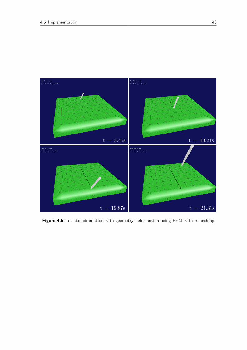
4.6 Implementation 40
t = 8.45s t = 13.21s
t = 21.31st = 19.87s
Figure 4.5: Incision simulation with geometry deformation using FEM with remeshing
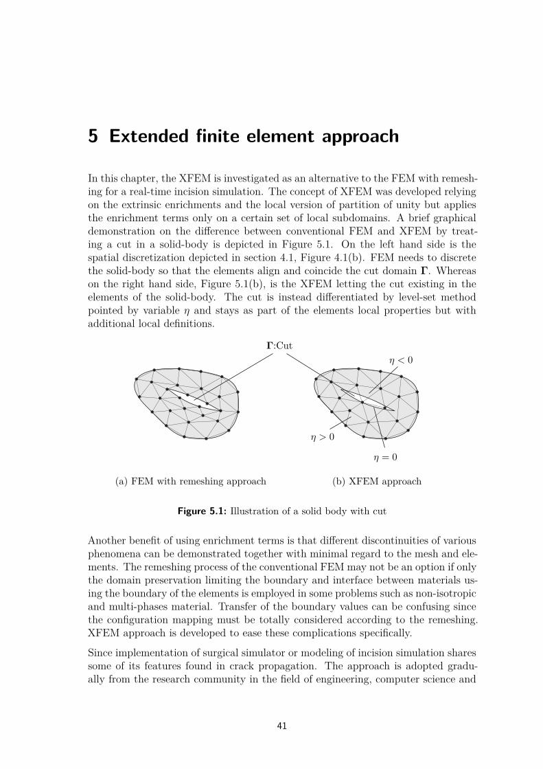
5 Extended finite element approach
In this chapter, the XFEM is investigated as an alternative to the FEM with remesh-ing for a real-time incision simulation. The concept of XFEM was developed relyingon the extrinsic enrichments and the local version of partition of unity but appliesthe enrichment terms only on a certain set of local subdomains. A brief graphicaldemonstration on the difference between conventional FEM and XFEM by treat-ing a cut in a solid-body is depicted in Figure 5.1. On the left hand side is thespatial discretization depicted in section 4.1, Figure 4.1(b). FEM needs to discretethe solid-body so that the elements align and coincide the cut domain Γ. Whereason the right hand side, Figure 5.1(b), is the XFEM letting the cut existing in theelements of the solid-body. The cut is instead differentiated by level-set methodpointed by variable η and stays as part of the elements local properties but withadditional local definitions.
Γ:Cut
η = 0
η < 0
η > 0
(a) FEM with remeshing approach (b) XFEM approach
Figure 5.1: Illustration of a solid body with cut
Another benefit of using enrichment terms is that different discontinuities of variousphenomena can be demonstrated together with minimal regard to the mesh and ele-ments. The remeshing process of the conventional FEM may not be an option if onlythe domain preservation limiting the boundary and interface between materials us-ing the boundary of the elements is employed in some problems such as non-isotropicand multi-phases material. Transfer of the boundary values can be confusing sincethe configuration mapping must be totally considered according to the remeshing.XFEM approach is developed to ease these complications specifically.
Since implementation of surgical simulator or modeling of incision simulation sharessome of its features found in crack propagation. The approach is adopted gradu-ally from the research community in the field of engineering, computer science and
41
5.1 Displacement approximation with discontinuities 42
medicine. Jeřábková exhibited an successful implementation of the surgical sim-ulator based on XFEM in her dissertation. Interesting is also the work presentedby Vigneron which discusses the deformation in a soft body as the result of bothsurgical cutting and tearing [96]. His works shows the ability of XFEM to considertwo discontinuities at the same time. This chapter is devoted to the discussion ontreating the incision or cut as a discontinuity in a solid material which is the back-ground principle of the XFEM approach. The approach will take the kinematic ofthe incision developed earlier in chapter 3 and derived the incision as part of thedisplacement discretization in element directly without considering the remeshingprocess. Since XFEM is actually the extended or variation of the conventional FEMdiscussed elaborately in chapter 4, some derivations and assumptions will be adoptedin this section with notices. The derivation and some illustrations regarding XFEMused in this chapter can also be reviewed from [16,39,46,58,63] if a more extensiveexplanation on the XFEM approach is required.
5.1 Displacement approximation with discontinuities
XFEM can be assumed to be a classical FEM capable of handling arbitrary strongand weak discontinuities [58]. The concept of XFEM is to enrich the approximationspaces so that it is capable of reproducing certain features of the problem of interest.The enrichments are applied only in a certain local sub-domain in order to increasethe order of completeness of the solution. In other words, it improves the accuracyof the approximation by including the information obtained from the analytical solu-tion in the local element domain directly. Employing XFEM in a simulation requiresinitially a conventional mesh similar to one from FEM. Then, during the simulation,the location of discontinuities are considered. Accordingly, new degrees of freedomare added to the conventional governing system of equations in the selected nodesnear the discontinuities.
Let consider the nodal reference configuration in a solid body X, also assumedis that a discontinuity is exhibited in an element of this solid body which has nnodes. The following displacement approximation uh is proposed by Belytschkoand Black for crack propagation simulation [14]. The formulation of the discretekinematics shall not be repeated but can be reviewed from section 4.1.
uh = ustd + uenr =n∑
j=1
Nj(X)uj +m∑
k=1
Nk(X)ψ(X)ak (5.1)
The first term of equation 5.1, ustd is recognized as the standard displacement ap-proximation seen in equation 4.7 of FEM. Where the second term, uenr refers to theadditional approximation or enrichment term due to discontinuity in the elementscontaining cut. uj is the nodal displacement vector of the regular degrees of free-dom found in the FEM. ak denotes the added set of DoFs m to the standard FEM.ψ(X) is the discontinuous enrichment function defined in the set of nodes near adiscontinuity.
5.2 Modeling of strong discontinuous fields 43
The enrichment functionψ(X), in general, can be chosen by applying an appropriateanalytical solution according to the type of discontinuity. It is the fact that differenttypes of phenomena require specific mathematic explanations. The shape functionof the enrichment term Nk is not required to be identical to that of the standardFEM Nj. It depends on the physical type of phenomena. In this work, it is assumedthat Nj = Nk and are identical to the shape functions for a tetrahedral element.
With the concept of XFEM, different and multiple types of discontinuity are allowedto be expressed in the same displacement approximation by adding just additionalterms coincide with the number and type of discontinuities as
uh =n∑
j=1
Nj(X)uj +np∑
l=1
m∑
k=1
Nk(X)ψl(X)alk (5.2)
with np denotes the number of discontinuities existing in the element. The originalmesh generated for the standard displacement approximation is mapped to the vec-tor u while the discontinuities are performed by the enrichment terms. The XFEMdoes not require the remeshing but instead employ an enrichment function for eachdiscontinuities. This is an advantage if the simulation involves in multiple cut inthe same element [46] or in an complicate interface problems such as the simulationof multi-phase flow where the material properties are changed gradually as they aremixed together [21,35].
5.2 Modeling of strong discontinuous fields
Incision, cut or crack are all considered to be one of strong discontinuities in anelement since it completely break the material bonds on both side of a cut plane.As mentioned earlier that modeling of a discontinuity in XFEM requires a properenrichment function suitable for a specific discontinuity.
To demonstrate the effect of enrichment functions, Figure 5.2 is brought to consideran one-dimensional deformation problem. The problem consists of three elementsand four nodes. Nj with j = 1, 2, 3, 4 are the shape functions satisfy the KroneckerDelta property and the Partition of Unity discussed in section 4.2. A strong discon-tinuity assumed to be a cut exists arbitrarily at Xc(η = 0) in the second element.The second element is therefore divided or separated into two bodies which is quan-titatively described as one staying above the cut (η > 0) and one staying below thecut (η < 0).
XFEM approach requires only the second element to be locally enriched. The en-richment affects accordingly second and third nodes, whereas first and forth nodesare not influenced by the cut and the enrichment does not required in these domains.The essential question is how to mathematically demonstrate the cut in the elementby choosing an enrichment function ψ(X) in equation 5.1. For a strong discontinu-ity such as the given example, two enrichment functions are often employed whichare the Heaviside and the Shifted functions.
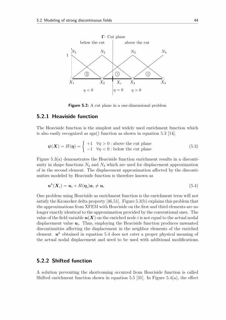
5.2 Modeling of strong discontinuous fields 44
2 3
η = 0η < 0 η > 0
Γ: Cut planeabove the cutbelow the cut
1
1N1 N2 N3 N4
X1 X2 X3 X4Xc
Figure 5.2: A cut plane in a one-dimensional problem
5.2.1 Heaviside function
The Heaviside function is the simplest and widely used enrichment function whichis also easily recognized as sgn() function as shown in equation 5.3 [14].
ψ(X) = H(η) =
+1 ∀η > 0 : above the cut plane−1 ∀η < 0 : below the cut plane
(5.3)
Figure 5.3(a) demonstrates the Heaviside function enrichment results in a disconti-nuity in shape functions N2 and N3 which are used for displacement approximationof in the second element. The displacement approximation affected by the disconti-nuities modeled by Heaviside function is therefore known as
uh(X i) = ui +H(ηi)ai 6= ui (5.4)
One problem using Heaviside as enrichment function is the enrichment term will notsatisfy the Kronecker delta property [46,51]. Figure 5.3(b) explains this problem thatthe approximations from XFEM with Heaviside on the first and third elements are nolonger exactly identical to the approximation provided by the conventional ones. Thevalue of the field variable u(X) on the enriched node i is not equal to the actual nodaldisplacement value ui. Thus, employing the Heaviside function produces unwanteddiscontinuities affecting the displacement in the neighbor elements of the enrichedelement. uh obtained in equation 5.4 does not cater a proper physical meaning ofthe actual nodal displacement and need to be used with additional modifications.
5.2.2 Shifted function
A solution preventing the shortcoming occurred from Heaviside function is calledShifted enrichment function shown in equation 5.5 [31]. In Figure 5.4(a), the effect
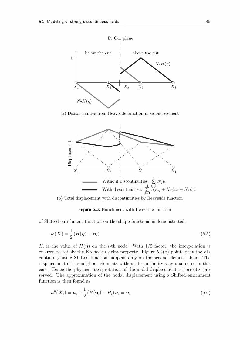
5.2 Modeling of strong discontinuous fields 45
Dis
plac
emen
t
Γ: Cut plane
above the cutbelow the cut1
N2H(η)
N3H(η)
X1
X1
X2
X2
X3
X3
X4
X4
Xc
(a) Discontinuities from Heaviside function in second element
(b) Total displacement with discontinuities by Heaviside function
Without discontinuities:4∑
j=1Njuj
With discontinuities:4∑
j=1Njuj +N2ψa2 +N3ψa3
Figure 5.3: Enrichment with Heaviside function
of Shifted enrichment function on the shape functions is demonstrated.
ψ(X) =1
2(H(η)−Hi) (5.5)
Hi is the value of H(η) on the i-th node. With 1/2 factor, the interpolation isensured to satisfy the Kronecker delta property. Figure 5.4(b) points that the dis-continuity using Shifted function happens only on the second element alone. Thedisplacement of the neighbor elements without discontinuity stay unaffected in thiscase. Hence the physical interpretation of the nodal displacement is correctly pre-served. The approximation of the nodal displacement using a Shifted enrichmentfunction is then found as
uh(X i) = ui +1
2(H(ηi)−Hi)ai = ui (5.6)
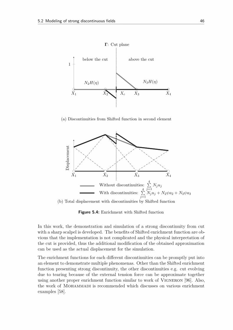
5.2 Modeling of strong discontinuous fields 46
Dis
plac
emen
t
Γ: Cut plane
above the cutbelow the cut1
N2H(η) N3H(η)
X1
X1
X2
X2
X3
X3
X4
X4
Xc
(a) Discontinuities from Shifted function in second element
(b) Total displacement with discontinuities by Shifted function
Without discontinuities:4∑
j=1Njuj
With discontinuities:4∑
j=1Njuj +N2ψa2 +N3ψa3
Figure 5.4: Enrichment with Shifted function
In this work, the demonstration and simulation of a strong discontinuity from cutwith a sharp scalpel is developed. The benefits of Shifted enrichment function are ob-vious that the implementation is not complicated and the physical interpretation ofthe cut is provided, thus the additional modification of the obtained approximationcan be used as the actual displacement for the simulation.
The enrichment functions for each different discontinuities can be promptly put intoan element to demonstrate multiple phenomenas. Other than the Shifted enrichmentfunction presenting strong discontinuity, the other discontinuities e.g. cut evolvingdue to tearing because of the external tension force can be approximate togetherusing another proper enrichment function similar to work of Vigneron [96]. Also,the work of Mohammadi is recommended which discusses on various enrichmentexamples [58].

5.3 Discrete governing system of equations with XFEM 47
5.3 Discrete governing system of equations withXFEM
Section 5.3 discusses on how to add the additional analytic solution to the dis-placement approximation and improve its completeness and accuracy. This analyticapproximation comes in form of the discontinuity enrichment function. For incisionsimulation, where the cut in a solid-body is treated by XFEM as a type of strongdiscontinuities, the Shifted enrichment approach is seen as a suitable solution andis adopted throughout the upcoming implementation in this work.
In order to obtain a discrete governing system of equations necessary for the ex-planation of the dynamic behavior of a solid-body, similar to the approach takenin section 4.2, the discrete kinematics with discontinuity derived in previous sec-tions will be considered while the kinematic of incision known from section 3 will berecalled again for XFEM derivation.
To begin with, the displacement approximation from equation 5.1 uh is rewritten inmatrix format as
uh =[
N ψN]
·
[
ustd
a
]
(5.7)
Vector uh puts together the standard approximation of the FEM ustd and adds theadditional DoFs a from the discontinuity approximation. In a similar manner, thestrain-displacement matrix B is extended to support these additional DoFs as
Bh =[
B ψB]
(5.8)
Considering Figure 5.5 gives a close perspective of the physical interpretation ex-plaining how XFEM approach works. In the Figure, a tetrahedral element withtotal volume V is cut arbitrarily and therefore divided into two volumes. Va andVb are referred to volume above the cut plane and volume below the cut plane re-spectively. Thus, to obtain an enriched element stiffness matrix kh(e), the integralfor the element stiffness matrix over total volume can accordingly be done sepa-rately [16,46]
kh(e) =∫
Ωe
(
Bh)TCBhdV =
∫
Va
(
Bh)TCBhdV +
∫
Vb
(
Bh)TCBhdV (5.9)
Substituting Bh from equation 5.8 and obtain
kh(e) =∫
Ωe
[
BT CB BT CψB
ψBT CB ψBT CψB
]
dV =
[
kuu(e) kua(e)
kau(e) kaa(e)
]
(5.10)
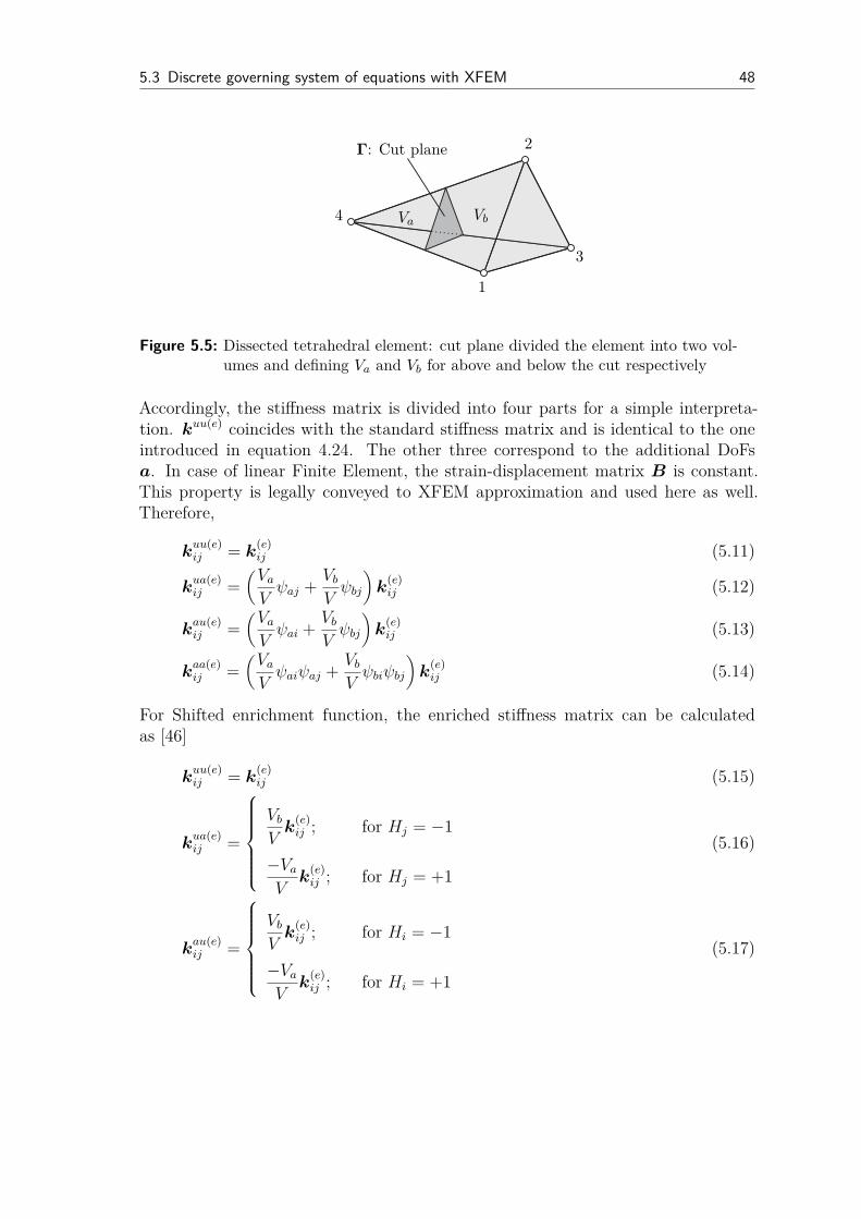
5.3 Discrete governing system of equations with XFEM 48
Va Vb
Γ: Cut plane
1
2
3
4
Figure 5.5: Dissected tetrahedral element: cut plane divided the element into two vol-umes and defining Va and Vb for above and below the cut respectively
Accordingly, the stiffness matrix is divided into four parts for a simple interpreta-tion. kuu(e) coincides with the standard stiffness matrix and is identical to the oneintroduced in equation 4.24. The other three correspond to the additional DoFsa. In case of linear Finite Element, the strain-displacement matrix B is constant.This property is legally conveyed to XFEM approximation and used here as well.Therefore,
kuu(e)ij = k
(e)ij (5.11)
kua(e)ij =
(
Va
Vψaj +
Vb
Vψbj
)
k(e)ij (5.12)
kau(e)ij =
(
Va
Vψai +
Vb
Vψbj
)
k(e)ij (5.13)
kaa(e)ij =
(
Va
Vψaiψaj +
Vb
Vψbiψbj
)
k(e)ij (5.14)
For Shifted enrichment function, the enriched stiffness matrix can be calculatedas [46]
kuu(e)ij = k
(e)ij (5.15)
kua(e)ij =
Vb
Vk
(e)ij ; for Hj = −1
−Va
Vk
(e)ij ; for Hj = +1
(5.16)
kau(e)ij =
Vb
Vk
(e)ij ; for Hi = −1
−Va
Vk
(e)ij ; for Hi = +1
(5.17)
5.3 Discrete governing system of equations with XFEM 49
kaa(e)ij =
Vb
Vk
(e)ij ; for Hi = Hj = −1
Va
Vk
(e)ij ; for Hi = Hj = +1
0; for Hi 6= Hj
(5.18)
As discussed in section 3.5, the incision promotes no total mass lost. Therefore,the expression of the enriched element mass matrix mh(e) is similar to that of theenriched stiffness matrix. The enriched shape function from equation 5.7 is appliedto the element mass matrix from equation 4.25 to obtain
mh(e) =∫
Ωe
[
N ψN]Tρ[
N ψN]
dV
=∫
Ωe
ρ
[
NN NψN
ψNN ψNψN
]
dV
=∫
Va
[
N ψN]Tρ[
N ψN]
dV +∫
Vb
[
N ψN]Tρ[
N ψN]
dV
=
[
muu(e) mua(e)
mau(e) maa(e)
]
(5.19)
For a linear Finite Element approximation, the shape functions are kept constantand allow the enriched element mass matrix to be integrated
muu(e)ij = m
(e)ij (5.20)
mua(e)ij =
Vb
Vm
(e)ij ; for Hj = −1
−Va
Vm
(e)ij ; for Hj = +1
(5.21)
mau(e)ij =
Vb
Vm
(e)ij ; for Hi = −1
−Va
Vm
(e)ij ; for Hi = +1
(5.22)
maa(e)ij =
Vb
Vm
(e)ij ; for Hi = Hj = −1
Va
Vm
(e)ij ; for Hi = Hj = +1
0; for Hi 6= Hj
(5.23)

5.3 Discrete governing system of equations with XFEM 50
Analogously, the element damping matrix can be calculated as of the FEM approachusing Rayleigh formulation. The derivation of damping is explicitly written as fol-low
duu(e)ij = a m
(e)ij + b k
(e)ij (5.24)
dua(e)ij =
Vb
Vd
(e)ij ; for Hj = −1
−Va
Vd
(e)ij ; for Hj = +1
(5.25)
dau(e)ij =
Vb
Vd
(e)ij ; for Hi = −1
−Va
Vd
(e)ij ; for Hi = +1
(5.26)
daa(e)ij =
Vb
Vd
(e)ij ; for Hi = Hj = −1
Va
Vd
(e)ij ; for Hi = Hj = +1
0; for Hi 6= Hj
(5.27)
The element nodal external forces are comprised with the discrete body force and thediscrete surface traction force, see section 4.2 equations 4.18 and 4.19. To supportthe additional DoFs a, the element nodal external forces are extended. Here arises adiscussion on how extended forces fh should be determined. Doing so, the derivationof an element nodal external forces is adopted while the standard shape function issubstituted with
[
N ψN]
. This yields
fh =[
fu fa]T
=∫
Ωe
[
N ψN]TρbdV +
∫
∂Ωe
[
N ψN]TT 0dA (5.28)
This approximation can be separately integrated on two volumes and surfaces usingthe earlier assumption. With constant shape functions for linear Finite Elementapproximation, the extended nodal external force is found as
fu(e)i = f
ext(e)i = m
uu(e)ij bi +
∫
Ωe
NiTi0dA (5.29)
fa(e)i =
Vb
Vm
(e)ij bi +
∫
Ab
NiTi0dA; for Hj = −1
−Va
Vm
(e)ij bi −
∫
Aa
NiTi0dA; for Hj = +1
0; for Hj 6= Hi
(5.30)
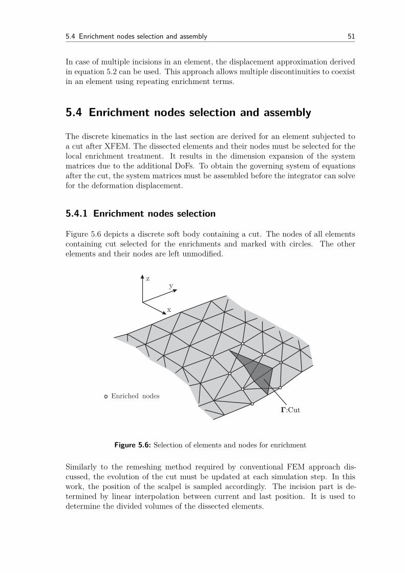
5.4 Enrichment nodes selection and assembly 51
In case of multiple incisions in an element, the displacement approximation derivedin equation 5.2 can be used. This approach allows multiple discontinuities to coexistin an element using repeating enrichment terms.
5.4 Enrichment nodes selection and assembly
The discrete kinematics in the last section are derived for an element subjected toa cut after XFEM. The dissected elements and their nodes must be selected for thelocal enrichment treatment. It results in the dimension expansion of the systemmatrices due to the additional DoFs. To obtain the governing system of equationsafter the cut, the system matrices must be assembled before the integrator can solvefor the deformation displacement.
5.4.1 Enrichment nodes selection
Figure 5.6 depicts a discrete soft body containing a cut. The nodes of all elementscontaining cut selected for the enrichments and marked with circles. The otherelements and their nodes are left unmodified.
Enriched nodes
z
x
y
Γ:Cut
Figure 5.6: Selection of elements and nodes for enrichment
Similarly to the remeshing method required by conventional FEM approach dis-cussed, the evolution of the cut must be updated at each simulation step. In thiswork, the position of the scalpel is sampled accordingly. The incision part is de-termined by linear interpolation between current and last position. It is used todetermine the divided volumes of the dissected elements.
5.4 Enrichment nodes selection and assembly 52
After nodes selection, the discontinuities are added to each shape functions of thedissected elements, while the calculation of extended terms in element stiffness, massand damping matrices are carried out. The additional DoFs are put into and extendthe displacement vector accordingly. Since the added DoFs are put purposefully toincrease the approximation accuracy, they coincide with the number of shape func-tions in an element required to be enhanced. If a tetrahedral element is thoroughlycut, all four shape functions are required to be enriched. Analogously, 12 additionalDoFs are necessary to enrich this element. For example, an element stiffness matrixis extended after a cut as
kh(e) =
kuu1,1 · · · kuu
1,12 kua1,1 · · · kua
1,12...
. . ....
.... . .
...kuu
12,1 · · · kuu12,12 kua
12,1 · · · kua12,12
kau1,1 · · · kau
1,12 kaa1,1 · · · kaa
1,12...
. . ....
.... . .
...kau
12,1 · · · kau12,12 kaa
12,1 · · · kaa12,12
∈ IR24×24 (5.31)
The same computation method can be applied to mass and damping matrices foreach tetrahedral element containing cut.
5.4.2 Assembly of enrichment DoFs
The added DoFs a as the consequence from the enriched nodes are staying as theextended approximation shown in equation 5.1 and 5.2. XFEM provides a systematicexpansion of the governing system of equations which requires only the a to stayright after the standard DoFs u. The assembly can be implemented to concentratestraightforwardly on these expanding regions.
The expansion in system matrices to support the additional DoFs is demonstrated bythe global stiffness matrixKh in equation 5.32. The dimension of the global stiffnessmatrix is extended dependently to the number of the dissected elements ncut. Since12 additional DoFs a are required for each completely dissected element, the dimen-sion of the global stiffness matrix can be calculated as IR(3nnode+12ncut)×(3nnode+12ncut).
Kh =
nele⋃
e=1
kuu(e)ncut⋃
k=1
kua(e)
ncut⋃
k=1
kau(e)ncut⋃
k=1
kaa(e)
∈ IR(3nnode+12ncut)×(3nnode+12ncut) (5.32)
The assembly process of the expanded stiffness matrix can be done by separate thestandard part to the extended parts. This yields great advantage as the standard
global stiffness matrix Kuu =nele⋃
e=1
= kuu(e) is computed only once during problem
initialization. It is preserved and remain unchanged for linear XFEM. The extendedparts are systematically and separately assembled before combined to Kuu to form
5.5 Dynamic simulation 53
a total enriched global stiffness matrix Kh. This procedure is also valid for enrichedglobal mass and damping matrices.
5.5 Dynamic simulation
After assembly process, the extended dynamic governing system of equations isobtained as presented in equation 5.33.
F h = Mhuh +Dhuh +Kuh (5.33)
or[
F ext
F a
]
=
[
Muu Mua
M au M aa
]
·¨
[
U
A
]
+
[
Duu Dua
Dau Daa
]
·˙
[
U
A
]
+
[
Kuu Kua
Kau Kaa
]
·
[
U
A
]
In order to solve for the solution, a proper integration is required. XFEM encountersno restriction to employ the Newmark Implicit Integration discussed in section 4.5.1.The integration on XFEM is rather straight forward. The Newmark Implicit Inte-gration parameters can also adopted without any necessity of modification from itsconventional setting from FEM in order to remain unconditionally stable.
Since XFEM approach does not alter the topology of the standard FEM part, theinitial boundary conditions applied earlier during initialization does not require anupdate to be mapped with the current topology. Similarly, the displacements uobtained from the integration can be mapped directly exhibits the actual geometryaffected to discontinuities without.
Another benefit of using XFEM is that the governing system of equations are re-versible to the origin state or any state back in time. This is viable due to thepreservation of the standard FEM part and systematic expansion of the governingsystem of equations. This can be an advantage if the evolution of the cut or adiscontinuity is history dependent.
5.6 Implementation
The implementation of the XFEM is similar to algorithm 2 of FEM. The simulationprocedures begin with the initialization or formulation of the simulation problem.In this regard, the XFEM can be initialized using a similar initialization algorithmto that of FEM. The material properties, Young’s modulus E, density ρ and Poissonratio ν must be provided.
The Lagrangian mesh generates the mesh topology which also determines the indexof displacement vector U and the number of elements found in the solid body. Theinitial Neumann and Dirichlet boundary conditions must be applied. The initialglobal mass Mh
0 , damping Dh0 and Kh
0 stiffness matrices can now be calculated.

5.6 Implementation 54
Without enrichment at the beginning of the simulation, these system matrices areidentical to Muu,Duu and Kuu.
The formulation of the dynamic system of governing equations is done so that theequation is ready to be solved using Newmark implicit integration method discussedin section 4.5.1.
It is worth to note that the initializations of FEM and XFEM can be shared dueto their similarity. XFEM can be considered a variation of the FEM simulation.Thus, if the simulations with both approaches are required, the implementation ina software can be done together without additional effort.
Algorithm 3: Initialization of XFEM simulation
Read material parameter:
E, ρ, νSimulation step indicator:
tn = 0 and n = 0Mesh generation: ←− BΓ at n = 0U , topology, number of elements nele
Apply initial boundary conditions:
Uϕ,0, Uϕ,0, Uϕ,0, F extt,0
Calculation initial system matrix:
Mh0 = Muu, Dh
0 = Duu, Kh0 = Kuu
Formulate dyn. governing system of equation: −→ equation 5.33
Algorithm 4 is the pseudo code of the incision simulation procedure using XFEM.During the simulation, the scalpel position rC ,n is read constantly at each simulationstep. If a collision between scalpel and the soft body is detected and the rate of cutevolution rC,n is not zero, the structural change Ξt : ΩΓ → BΓ will be determined.The nodes of the dissected elements during the last simulation step must be selectedand enriched. In this work, the elements are only allowed to be cut thoroughly. Thus,the number of additional DoFs a depends on the number of dissected elements asdiscussed in section 5.4.1.
The displacement vector Uhn and the enriched force vector F h
n are extended addingthe a after its highest indexes. Accordingly, the enriched element mass, damping,stiffness and nodal forces of each dissected elements are computed and assembled toupdate the global matrices Mh
n, Dhn, Kh
n and F hn to the current simulation step.
In case, the collision between the scalpel tip and the soft body does not occur or therC,n is zero, it is implied that the structural change Ξt = 0 at the current simulationstep. Therefore, the system matrices and nodal external forces of the last simulationstep are adopted as the current system matrices since they are identical.
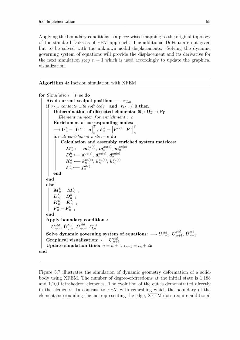
5.6 Implementation 55
Applying the boundary conditions is a piece-wised mapping to the original topologyof the standard DoFs as of FEM approach. The additional DoFs a are not givenbut to be solved with the unknown nodal displacements. Solving the dynamicgoverning system of equations will provide the displacement and its derivative forthe next simulation step n + 1 which is used accordingly to update the graphicalvisualization.
Algorithm 4: Incision simulation with XFEM
for Simulation = true do
Read current scalpel position: −→ rC,n
if rC,n contacts with soft body and rC,n 6= 0 then
Determination of dissected elements: Ξt : ΩΓ → BΓ
Element number for enrichment : eEnrichment of corresponding nodes:
−→ Uhn =
[
U std a]T
n, F h
n =[
F ext F a]T
n
for all enrichment node := e do
Calculation and assembly enriched system matrices:
Mhn ←−m
ua(e)n , m
au(e)n , m
au(e)n
Dhn ←− d
ua(e)n , dau(e)
n , dau(e)n
Khn ←− k
ua(e)n , kau(e)
n , kau(e)n
F hn ←− f
a(e)n
end
end
else
Mhn = Mh
n−1
Dhn = Dh
n−1
Khn = Kh
n−1
F hn = F h
n−1
end
Apply boundary conditions:
U stdϕ,n, U
stdϕ,n, U
stdϕ,n, F
extt,n
Solve dynamic governing system of equations: −→ U stdn+1, U
stdn+1, U
stdn+1
Graphical visualization: ←− U stdn+1
Update simulation time: n = n+ 1, tn+1 = tn +∆t
end
Figure 5.7 illustrates the simulation of dynamic geometry deformation of a solid-body using XFEM. The number of degree-of-freedoms at the initial state is 1,188and 1,100 tetrahedron elements. The evolution of the cut is demonstrated directlyin the elements. In contrast to FEM with remeshing which the boundary of theelements surrounding the cut representing the edge, XFEM does require additional
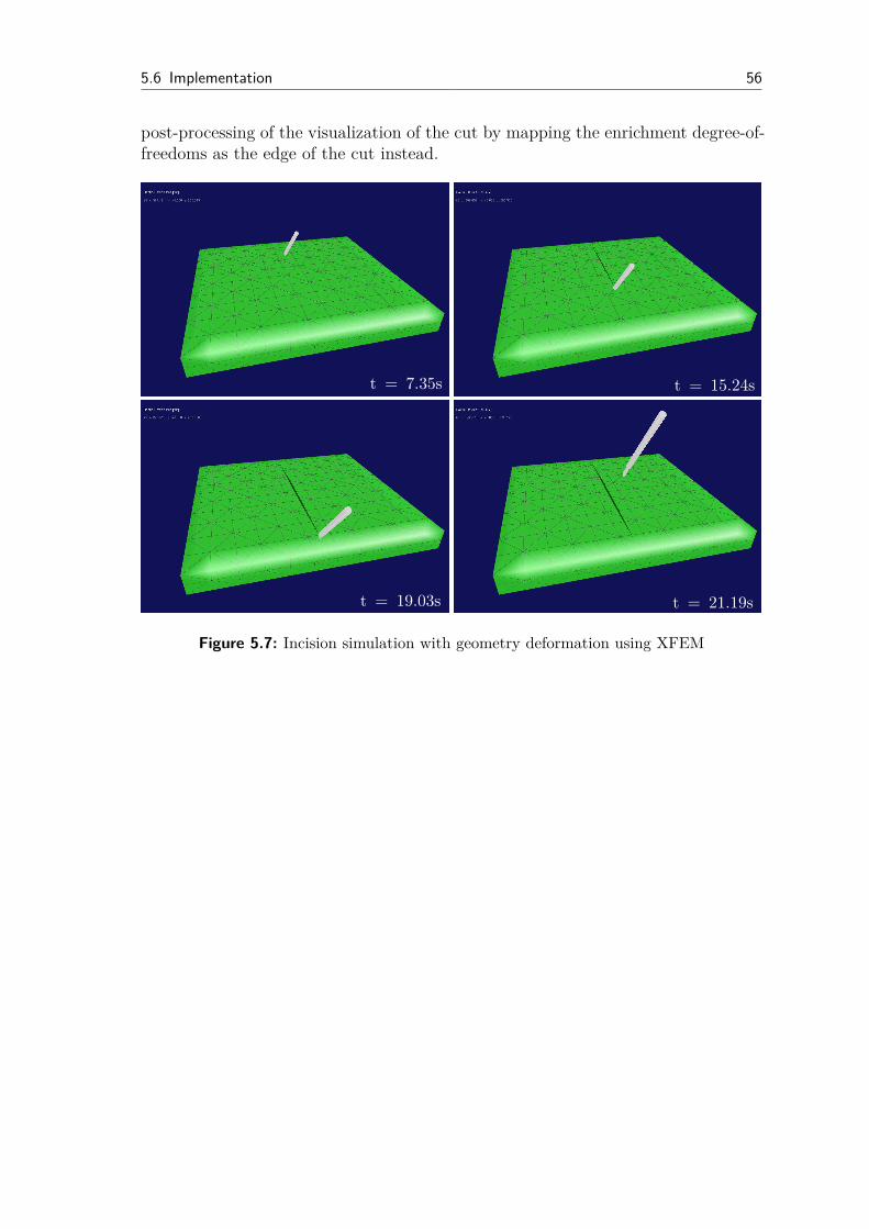
5.6 Implementation 56
post-processing of the visualization of the cut by mapping the enrichment degree-of-freedoms as the edge of the cut instead.
t = 7.35s t = 15.24s
t = 21.19st = 19.03s
Figure 5.7: Incision simulation with geometry deformation using XFEM
6 Remarks on implementation practicality
A practical modeling of a soft body in fast transient applications such as the incisionprocess is a major challenge of this work. It is because the simulation is aimed tobe used as a contact model for telepresence application. Obviously, the real-timevisualization capability must be obtained. Two approaches are proposed, FEM andXFEM. This chapter will discuss on their practicalities as a developing tool of acontact model.
6.1 Finite element method with remeshing
FEM is appointed to demonstrate the dissection of elements when a cut is exhibited.Doing so the Lagrange mesh which is fixed to specific material points must bereconsidered. An example remeshing algorithm from section 4.4.1 is employed forthis task to handle a mesh condition which represents the actual geometry of the softbody at each simulation step. The remeshing algorithm in this work is developedto constrain the incision on a single vertical plane and only between the nodes.As a result, the topology of the governing system of equations is changed and thedimension of system matrices is expanded to associate the increasing number of DoFsfrom the additional nodes surrounding the cut. The dynamic governing system ofequations is required to be reassembled similarly to the initializing of the simulation.Applying the boundary conditions are subjected to rearranged topology. Thus, theremapping before applying the boundary conditions from the predecessor to thecurrent configuration must be made.
It must be noted that, for a general case, the implementation efficiency of FEM foran incision simulation depends strongly on the corporate remeshing algorithm. Ifthe incision was made in the middle of the elements, the number of added elementsmay not be zero since remeshing algorithm must substitute the dissected tetrahedronelements with generally smaller ones [19,49]. Thus, the computing resources can notbe guaranteed. This can be critical for an application of the contact model in anactual telepresence scenario where a stable operation with limit computing resourcesis required.
Another important aspect of the FEM is the discretization shall be done so that thevalidity of the governing system of equations in an element is preserved. If a propertyin an element is altered, the Lagrangian mesh must be reconsidered. This can be anissue for a complex mechanics problem which deals with multi discontinuities at thesame time due to the mesh condition. A good example is the FEM analysis of hotcracking using temperature-dependent interface of Shibahara et al. [77, 78].
57
6.2 Extended finite element method 58
On the other hand, as an advantage, the remeshing provides a clear interface sepa-ration between continuous domains and a discontinuity. For an incision simulation,the edge of elements represent the edge of cut indicatively and require no post-processing for the visualization. The interaction with an external force asserted ona node of the edge of the cut can be treated as the Neumann boundary conditionsof that current simulation step.
6.2 Extended finite element method
XFEM was originally developed to deal with a complex discontinuity with interfacewith a minimum consideration of the mesh conditions [14]. XFEM uses the extrinsicenrichments and the local version of partition of unity but apply the enrichmentterms only on a certain set of local subdomains. The local subdomains are selectedcoinciding with the element containing cut.
The enrichment for the incision simulation is the Shifted function in this work. Itendorses the internal dissection in an element with the local enrichment DoFs. As aresult, the governing system of equations, is expanded to support additional DoFsas discussed in section 5.4. Although the expansion due to enrichment is done, theassembly process does not inquire a complete rebuild of the system matrices butonly for the extended quadrants. The additional DoFs are allowed to be arrangedafter the highest index of the displacement vector instead of being as constituentvariables among the original DoFs done by FEM with remeshing.
The remapping of boundary conditions is not necessary due to the unaltered La-grangian mesh. The original nodes stay attached to the same material points sincethe initialization. It eases the treatment of boundary conditions significantly. Thesenature characteristics of XFEM approach provide an advantage in computing re-source management. Because a discontinuity is systematically added to the systemmatrices, therefore the necessary computing resource can be calculated precisely.Also, if required, the already-added discontinuities can be taken out by neglectingthe corresponding additional DoFs. Thus, the idea of enrichment enables the reversalof the system matrices to any previous configuration.
A disadvantage of XFEM is where the FEM with remeshing fulfills. The visualiza-tion of the edge of the cut does not explicitly demonstrated by XFEM and requiresan extra post-processing. This is because the cut is treated in the local element do-mains and not in a global one. If the tetrahedron elements are small enough, textsc-Jeřábková uses the edge of tetrahedron elements subjected to the cut to visualizationthe approximated cut [46]. In this work, a linear is draw in the dissected elementsas the visualization of the cut in the body as the scalpel is traveling through them.Moreover, if the interaction with the edge of cut is required, XFEM will meets itsshortcoming if additional interpretation is not utilized due to lacking of true nodeson the edge of the cut.
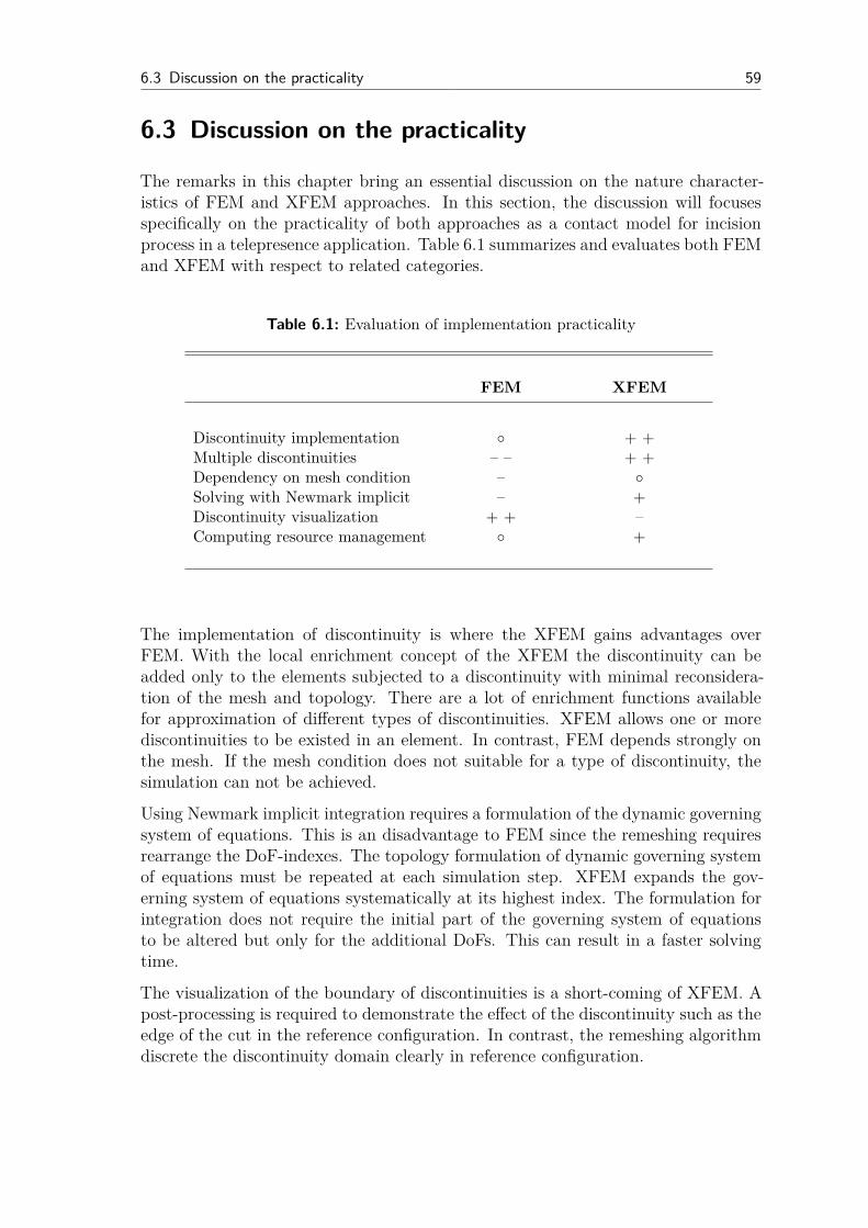
6.3 Discussion on the practicality 59
6.3 Discussion on the practicality
The remarks in this chapter bring an essential discussion on the nature character-istics of FEM and XFEM approaches. In this section, the discussion will focusesspecifically on the practicality of both approaches as a contact model for incisionprocess in a telepresence application. Table 6.1 summarizes and evaluates both FEMand XFEM with respect to related categories.
Table 6.1: Evaluation of implementation practicality
FEM XFEM
Discontinuity implementation + +Multiple discontinuities – – + +Dependency on mesh condition – Solving with Newmark implicit – +Discontinuity visualization + + –Computing resource management +
The implementation of discontinuity is where the XFEM gains advantages overFEM. With the local enrichment concept of the XFEM the discontinuity can beadded only to the elements subjected to a discontinuity with minimal reconsidera-tion of the mesh and topology. There are a lot of enrichment functions availablefor approximation of different types of discontinuities. XFEM allows one or morediscontinuities to be existed in an element. In contrast, FEM depends strongly onthe mesh. If the mesh condition does not suitable for a type of discontinuity, thesimulation can not be achieved.
Using Newmark implicit integration requires a formulation of the dynamic governingsystem of equations. This is an disadvantage to FEM since the remeshing requiresrearrange the DoF-indexes. The topology formulation of dynamic governing systemof equations must be repeated at each simulation step. XFEM expands the gov-erning system of equations systematically at its highest index. The formulation forintegration does not require the initial part of the governing system of equationsto be altered but only for the additional DoFs. This can result in a faster solvingtime.
The visualization of the boundary of discontinuities is a short-coming of XFEM. Apost-processing is required to demonstrate the effect of the discontinuity such as theedge of the cut in the reference configuration. In contrast, the remeshing algorithmdiscrete the discontinuity domain clearly in reference configuration.
6.3 Discussion on the practicality 60
An ability to spontaneous model an unfamiliar object is a general requirement fora contact model in a telepresence application. The contact model must be ableto simulate every actual contact mechanics in the remote environment. Moreover,the contact model should be efficient enough to guarantee its real-time simulationcapability. This can be achieved with the necessary of hardware resource planedbefore hand. As discussed earlier, XFEM provides a range of flexibility how tomodel a contact mechanics with discontinuities. The maximum of memory requiredto store the dynamic governing of equations can be precisely calculated from thenumber of elements and the number of interested discontinuities. FEM depends onthe remeshing algorithm to management the computing resources.
Considering XFEM is indeed developed from the conventional FEM, XFEM main-tains the characteristic and the benefits of FEM but yet with extended capabilities.XFEM does prove the enrichment strategy suits better as a developing tool for amedical contact model because of its range of modeling flexibilities.
7 Adaptive empirical incision force model
A contact model is required to render both the visualization of the geometry de-formation and the incision force for the haptic force feedback. FEM and XFEMdiscussed in the earlier sections demonstrate the geometry deformation of a solidbody during incision indicatively. The incision forces can not be calculated from thegoverning system of equations derived from both approaches. Instead, they must begiven as part of the Neumann boundary conditions acting on nodes of the dissectedelement where the scalpel is staying. Both FEM and XFEM require these boundaryconditions to be solvable by the integrator. To render the incision force for the hap-tic feedback perception and to fulfill the required Neumann boundary conditions,an incision force model is empirically developed in this work based on the frictionmodel in section 7.1.
However, the incision force involves in various variables and depends strongly onthe situation, accurate rendered forces from a friction model may not be imminentwhile the friction coefficients remain constant throughout the incision process. Insection 7.2, the adaptive parameter identification algorithm is developed. It verifiesconstantly the simulated feedback force to the actual force measurements from theforce sensor and instantly adjusts the coefficients in the incision force model.
As the third algorithm, in section 7.3, an optimization algorithm is introduced todetermine a set of optimum control parameters which guarantees a stable adaptationof the adaptive parameter identification algorithm.
7.1 Force modeling of haptic incision perception
The early implementation of force model for haptic force feedback rendering is thespring-damping such as the works of Terzopoulos et al. [91], Jeřábková [46]and Sela et al. [74]. This model is simple and allow the human operator a senseof contact force. However, this implementation does not valid for the incision forcedue to an incorrect physical interpretation.
In Figure 7.1, the incision force F Incision is demonstrated to be the resisting forceacting on the scalpel surfaces as the scalpel travels through the solid body in theincision direction. C denotes the current scalpel tip, which is pointed by vector rC .Vector r0 refers to the reference point where the incision begins.
In section 3, Figure 3.1, the definition of the cut in a solid-body is made, pointingthat the normal vector nt is the direction of the cut whereas the vector na is per-pendicular to the cut direction and to the vector nt. Therefore, the cut evolution
61
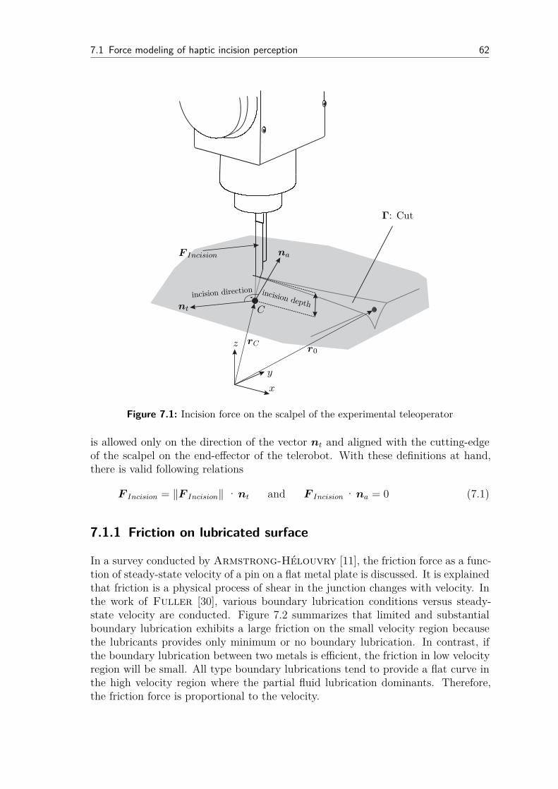
7.1 Force modeling of haptic incision perception 62
F Incision
incision depthincision direction
C
Γ: Cut
nt
na
r0rC
x
y
z
Figure 7.1: Incision force on the scalpel of the experimental teleoperator
is allowed only on the direction of the vector nt and aligned with the cutting-edgeof the scalpel on the end-effector of the telerobot. With these definitions at hand,there is valid following relations
F Incision = ‖F Incision‖ ·nt and F Incision ·na = 0 (7.1)
7.1.1 Friction on lubricated surface
In a survey conducted by Armstrong-Hélouvry [11], the friction force as a func-tion of steady-state velocity of a pin on a flat metal plate is discussed. It is explainedthat friction is a physical process of shear in the junction changes with velocity. Inthe work of Fuller [30], various boundary lubrication conditions versus steady-state velocity are conducted. Figure 7.2 summarizes that limited and substantialboundary lubrication exhibits a large friction on the small velocity region becausethe lubricants provides only minimum or no boundary lubrication. In contrast, ifthe boundary lubrication between two metals is efficient, the friction in low velocityregion will be small. All type boundary lubrications tend to provide a flat curve inthe high velocity region where the partial fluid lubrication dominants. Therefore,the friction force is proportional to the velocity.
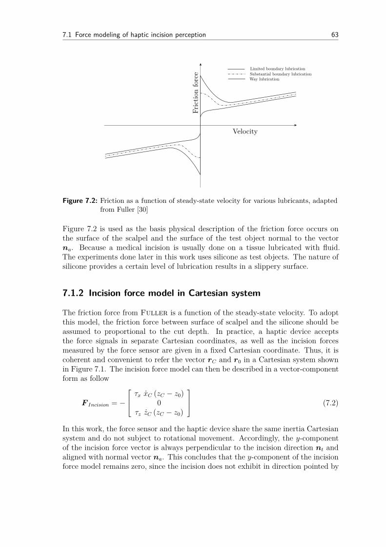
7.1 Force modeling of haptic incision perception 63
Fri
ctio
nfo
rce
Velocity
Limited boundary lubricationSubstantial boundary lubricationWay lubrication
Figure 7.2: Friction as a function of steady-state velocity for various lubricants, adaptedfrom Fuller [30]
Figure 7.2 is used as the basis physical description of the friction force occurs onthe surface of the scalpel and the surface of the test object normal to the vectorna. Because a medical incision is usually done on a tissue lubricated with fluid.The experiments done later in this work uses silicone as test objects. The nature ofsilicone provides a certain level of lubrication results in a slippery surface.
7.1.2 Incision force model in Cartesian system
The friction force from Fuller is a function of the steady-state velocity. To adoptthis model, the friction force between surface of scalpel and the silicone should beassumed to proportional to the cut depth. In practice, a haptic device acceptsthe force signals in separate Cartesian coordinates, as well as the incision forcesmeasured by the force sensor are given in a fixed Cartesian coordinate. Thus, it iscoherent and convenient to refer the vector rC and r0 in a Cartesian system shownin Figure 7.1. The incision force model can then be described in a vector-componentform as follow
F Incision = −
τx xC (zC − z0)0
τz zC (zC − z0)
(7.2)
In this work, the force sensor and the haptic device share the same inertia Cartesiansystem and do not subject to rotational movement. Accordingly, the y-componentof the incision force vector is always perpendicular to the incision direction nt andaligned with normal vector na. This concludes that the y-component of the incisionforce model remains zero, since the incision does not exhibit in direction pointed by

7.1 Force modeling of haptic incision perception 64
vector na. The incision force model is a function of the cutting velocity (x or z)depending on cut direction and the cut-depth (zC − z0).
With incision force model, the haptic force feedback rendering at a high-samplingrate is assuaged. The coefficients τ has unit of Ns/m2 have the most crucial rolefor a precise incision force prediction. It is related not only to the friction coefficientbut also depends on the geometry of the employed scalpel. For example, τx relatesto the cutting edge of the scalpel, whereas τz to its the sharp end. If a scalpel witha sharp end similar to one in Figure 7.1 is employed, it is assumable that τz shouldsmaller than τx since the object introduces a smaller resisting force as it is beingpierced.
3 4 5 6 7 8 9-1
0
1
2
3
4
5
3 4 5 6 7 8 9-3
-2
-1
0
1
2
3
3 4 5 6 7 8 9-20
-10
0
10
3 4 5 6 7 8 9-100
-50
0
50
Begin End
Fx(N
)F
e,x(N
)
time(s)
Cut
-dep
th(mm
)C
utti
ngve
loci
ty:x
(mm/s
)
Measurement: Fm,x
Prediction: FIncision,x
Figure 7.3: Comparison of the measured and the predicted incision forces in horizontaldirection align with the x-direction with constant τx = −2× 10⁻³ Ns
m2
For an explanation of the empirical incision force model, Figure 7.3 and 7.4 shallbe discussed. Both demonstrate the results obtained from an experiment whichundergoes an incision process in a silicone test object. The measured incision forcesin x and z-directions were obtained using a force sensor at the end-effector of theteleoperator. Simultaneously, the empirical incision force model from Equation 7.2

7.1 Force modeling of haptic incision perception 65
computed the incision force according to the scalpel position in the silicone testobject with the arbitrarily constant coefficients τx = τz = −2× 10⁻³ Ns/m2. Theincision began when the tip of the scalpel pierced through the surface of the testobject which can be noticed from the change in cut-depth. The scalpel was thereforedrawn in the negative x-direction to exhibit a cut in the test object with an almostconstant cut-depth before ended by pulling the scalpel out of the test object.
In Figure 7.3, the measured incision force Fm,x is plotted against the cut-depthand cutting velocity. It is obvious, as proposed, that the measured incision force isproportional to the cut-depth and the cut-velocity as the scalpel travels through theobject in −x-direction. On the other hand, the predicted incision force FIncision,x
provides a similar result with the aspects of incision process are presented correctly.However, a smaller magnitude is noticed due to an incorrect value of coefficient τx.The force error Fe,x reveals that the error between the measured and the predictedforces is not constant during the incision process which points that coefficient τx
can not be a constant. This can be explained using the friction-velocity curve fromFigure 7.2 that the friction coefficient is not proportional throughout the velocityregion. The horizontal incision force in x-direction is foremost important for thehaptic perception, since it demonstrates the haptic perception of the resisting forceas the scalpel travels through the test object.
In Figure 7.4, the empirical incision force model was again employed to predictthe incision force for the z-direction of the same experiment as previous. The z-component of the incision force is mostly noticeable when the cut-depth is changedor during piercing and pulling the scalpel out of the test object. This verticalincision force perception is especially critical during the first impact with the testobject. Similar as of previous, the incision force model demonstrated the piercingforce occurring during the first impact of the sharp end of the scalpel with the testobject as well as the friction force acting on the scalpel surface as the scalpel waspulled out. The magnitude of the predicted incision force in z-direction FIncision,z
was larger than the measured one. This convinces that the given coefficient τz isobviously inaccurate. In the same manners as of the x-direction, the force error Fe,z
was not constant pointing to the fact that the coefficient τz shall not remain as aconstant throughout the incision process.
A teleoperator is often controlled by hands of its human operator using a haptic de-vice. An inaccurate coefficient τ can cause the human operator a false decision anddamages the remote environment. An accurate perception without a distortion istherefore required. However, actual telepresence applications are usually appointedto work in a unknown environment and conditions. Therefore, for a medical telep-resence system, the incision is mostly done to an object which its characteristic maybe unknown. Accordingly, the coefficient τ in the incision force model must be as-sumed to be unknown in the first place. τ can be theoretically predetermined foreach material and object found in the remote environment. Nevertheless, this off-line parameter identification may not be practical or functional in the environmentwhich changes rapidly or there is an uncertainty in the material type. An adaptiveparameter identification algorithm, discussed in the next section is one of a logical
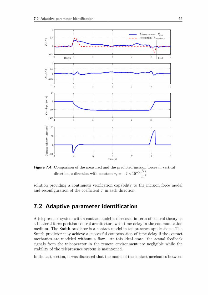
7.2 Adaptive parameter identification 66
3 4 5 6 7 8 9-0.5
0
0.5
1
3 4 5 6 7 8 9-1
-0.5
0
0.5
1
3 4 5 6 7 8 9-20
-10
0
10
3 4 5 6 7 8 9-50
0
50
100
Begin End
Fz(N
)F
e,z(N
)
time(s)
Cut
-dep
th(mm
)C
utti
ngve
loci
ty:z
(mm/s
)
Measurement: Fm,z
Prediction: FIncision,z
Figure 7.4: Comparison of the measured and the predicted incision forces in vertical
direction, z direction with constant τz = −2× 10⁻³ Ns
m2
solution providing a continuous verification capability to the incision force modeland reconfiguration of the coefficient τ in each direction.
7.2 Adaptive parameter identification
A telepresence system with a contact model is discussed in term of control theory asa bilateral force-position control architecture with time delay in the communicationmedium. The Smith predictor is a contact model in telepresence applications. TheSmith predictor may achieve a successful compensation of time delay if the contactmechanics are modeled without a flaw. At this ideal state, the actual feedbacksignals from the teleoperator in the remote environment are negligible while thestability of the telepresence system is maintained.
In the last section, it was discussed that the model of the contact mechanics between

7.2 Adaptive parameter identification 67
teleoperator and its remote environment must be determined before the initializa-tion of a teleoperation. However, the correct modeling and identification of theenvironment are achievable only in some particular situations and not in general.In fact, it is arguable that the concept of Smith predictor discussed in chapter 2can actually be realized in a genuine telepresence application and scenario. As adefensive argument, in this work, the incision force model in equation 7.2 can becontinuously validated during the actual incision.
Operator
EmpiricalIncisionForce
Model
HapticDevice
Delayed Communication:
Teleoperator
RemoteEnvironment
PI-Controller
− +
+
+ rC,H rC,He−sT
rCF Incision
Fm
FH
F ∗e
∆τ
F Incisione−2sT Fme
−sT
e−sT
e−2sT
Figure 7.5: Adaptive incision force model algorithm in a telepresence system
Figure 7.5 demonstrates a proposed control loop for a telepresence system. Theteleoperator is deployed to the remote environment whereas its human operator con-trols it from a local station using a haptic device. The human operator actuates thehaptic device providing a force vector FH allowing the haptic device to register thereference position of the teleoperator end-effectorrC,H . This position commands arepassed through a delayed communication with an assumed constant time delay T tothe teleoperator. The movement of the teleoperator is depicted by the actual posi-tion of its end-effector rC . The contact and interaction with the remote environmentprovides a contact force Fm which is measurable with a force sensor. Fm is requiredto be fed back via the same delayed communication to the local station where thehuman operator exists. For a conventional telepresence system, due to time delayof the close-loop, the arrival of Fm at the human operator will be 2T later after thereference position rC is sent. Therefore, the time delay leads to an unsynchronizedforce-position relation at the human operator. The phenomena results in a unrealis-tic experience which may cause the human operator a false decision because of thereaction to the feedback with phase shift.
There are some implementations of Smith predictor which do not neglect the delayedfeedback signal. On the other hand, the proposed control loop does not allow the
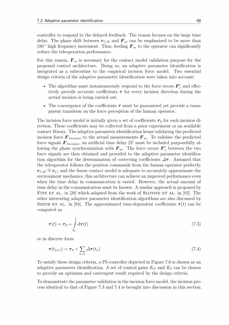
7.2 Adaptive parameter identification 68
controller to respond to the delayed feedback. The reason focuses on the large timedelay. The phase shift between rC,H and Fm can be emphasized to be more than180 high frequency movement. Thus, feeding Fm to the operator can significantlyreduce the teleoperation performance.
For this reason, Fm is necessary for the contact model validation purpose for theproposed control architecture. Doing so, an adaptive parameter identification isintegrated as a subroutine to the empirical incision force model. Two essentialdesign criteria of the adaptive parameter identification were taken into account:
• The algorithm must instantaneously respond to the force errors F ∗
e and effec-tively provide accurate coefficients τ for every incision direction during theactual incision is being carried out.
• The convergence of the coefficients τ must be guaranteed yet provide a trans-parent transition on the force perception of the human operator.
The incision force model is initially given a set of coefficients τ 0 for each incision di-rection. These coefficients may be collected from a prior experiment or an availablecontact library. The adaptive parameter identification keeps validating the predictedincision force F Incision to the actual measurements Fm. To validate the predictedforce signals F Incision, an artificial time delay 2T must be included purposefully al-lowing the phase synchronization with Fm. The force errors F ∗
e between the twoforce signals are then obtained and provided to the adaptive parameter identifica-tion algorithm for the determination of correcting coefficients ∆τ . Assumed thatthe teleoperator follows the position commands from the human operator perfectly,rC,H
∼= rC , and the linear contact model is adequate to accurately approximate theenvironment mechanics, this architecture can achieve an improved performance evenwhen the time delay in communication is varied. However, the actual amount oftime delay in the communication must be known. A similar approach is proposed byFite et al. in [28] which adapted from the work of Slotine et al. in [82]. Theother interesting adaptive parameter identification algorithms are also discussed bySmith et al. in [84]. The approximated time-dependent coefficients τ (t) can becomputed as
τ (t) = τ 0 +
t∫
t0
dτ (t) (7.3)
or in discrete form
τ (tn+1) = τ 0 +∑
n=1
∆τ (tn) (7.4)
To satisfy these design criteria, a PI-controller depicted in Figure 7.6 is chosen as anadaptive parameter identification. A set of control gains KP and KI can be chosento provide an optimum and convergent result required by the design criteria.
To demonstrate the parameter validation in the incision force model, the incision pro-cess identical to that of Figure 7.3 and 7.4 is brought into discussion in this section.
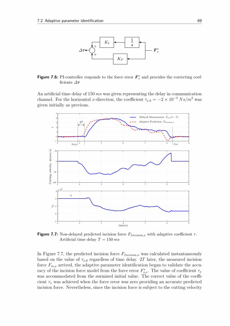
7.2 Adaptive parameter identification 69
+
+F ∗
e∆τ
KP
KI1s
Figure 7.6: PI-controller responds to the force error F ∗e and provides the correcting coef-
ficients ∆τ
An artificial time delay of 150ms was given representing the delay in communicationchannel. For the horizontal x-direction, the coefficient τx,0 = −2× 10⁻³ Ns/m2 wasgiven initially as previous.
3 4 5 6 7 8 9-1
0
1
2
3
4
5
F
3 4 5 6 7 8 9-8
-6
-4
-2
0x 10
-3
3 4 5 6 7 8 9-100
-50
0
50
Begin
t0
End
time(s)
2T
Cut
ting
velo
city
:x
(mm/s
)τ x
Delayed Measurement: Fm,x(t− T )
Adaptive Prediction: FIncision,x
Figure 7.7: Non-delayed predicted incision force FIncision,x with adaptive coefficient τ .Artificial time delay T = 150ms
In Figure 7.7, the predicted incision force FIncision,x was calculated instantaneouslybased on the value of τx,0 regardless of time delay. 2T later, the measured incisionforce Fm,x arrived, the adaptive parameter identification began to validate the accu-racy of the incision force model from the force error F ∗
x,e. The value of coefficient τx
was accommodated from the surmised initial value. The correct value of the coeffi-cient τx was achieved when the force error was zero providing an accurate predictedincision force. Nevertheless, since the incision force is subject to the cutting velocity

7.2 Adaptive parameter identification 70
x, the coefficient τx remained being adjusted until the end of the scalpel penetrationin the test object. The obvious difference of coefficient τx in high and low cuttingvelocity regions is demonstrated which confirms Figure 7.2.
3 4 5 6 7 8 9-1
-0.5
0
0.5
1
F
3 4 5 6 7 8 9-3
-2.5
-2
-1.5
-1
-0.5
0x 10
-3
3 4 5 6 7 8 9-50
0
50
100
Begin End
t0
time(s)
2T
Cut
ting
velo
city
:z
(mm/s
)τ z
Delayed Measurement: Fm,z(t− T )
Adaptive Prediction: FIncision,z
Figure 7.8: Non-delayed predicted incision force FIncision,z with adaptive coefficient τ .Artificial time delay T = 150ms
Similarly, in Figure 7.8, the incision force in vertical z-direction was predicted withan identical initial value of coefficient τz,0 = −2× 10⁻³ Ns/m2. The incision forcemodel reacted on the collision of the scalpel tip with the test object and calculatean amount of the feedback force using predefined τz,0. The adaptive parameteridentification began to correct to obtain the actual value of the coefficient τz asstated by equation 7.3 and 7.4. The final value of τz is not identical and smallerthan that of τx which is consistent with the assumption that τ is scalpel-geometrydependent. Hence, τ for each incision direction can be varied.
For a discussion on the accuracy improvement of the incision force model, the pre-dicted incision force FIncision,x is purposively delayed by 2T in Figure 7.9. This allowsa direct magnitude comparison of the predicted incision force and the measurement.FIncision,x is apparently more accurate with adaptive parameter identification algo-rithm when compared to the earlier results without adaptation in Figure 7.3.

7.2 Adaptive parameter identification 71
3 4 5 6 7 8 9-1
0
1
2
3
4
5
3 4 5 6 7 8 9-3
-2
-1
0
1
2
3
Fx(N
)F
∗ e,x(N
)
time(s)
Delayed Measurement: Fm,x(t− T )
Adaptive Prediction: FIncision,x(t− 2T )
Figure 7.9: Incision force error F ∗e,x shows an accuracy improvement with adaptive pa-
rameter identification algorithm in the horizontal direction
In the same manner, Figure 7.10 demonstrates an improvement of the prediction overone without the adaptive parameter identification algorithm depicted in Figure 7.4.This is a useful benefit of having the adaptive parameter identification algorithmsince it allows an approximate model parameter to be existed in the beginning whilethe correction can be made when a necessity arises. The use of PI-controller asthe adaptive parameter identification provides a transparent correction to the forcefeedback rendering while the natural presentation of the incision force is preserved.
3 4 5 6 7 8 9-1
-0.5
0
0.5
1
3 4 5 6 7 8 9-1
-0.5
0
0.5
1
Fz(N
)F
∗ e,z(N
)
time(s)
Delayed Measurement: Fm,z(t− T )
Adaptive Prediction: FIncision,z(t− 2T )
Figure 7.10: Incision force error F ∗e,z in the vertical direction also declines when the
adaptive parameter identification algorithm is employed
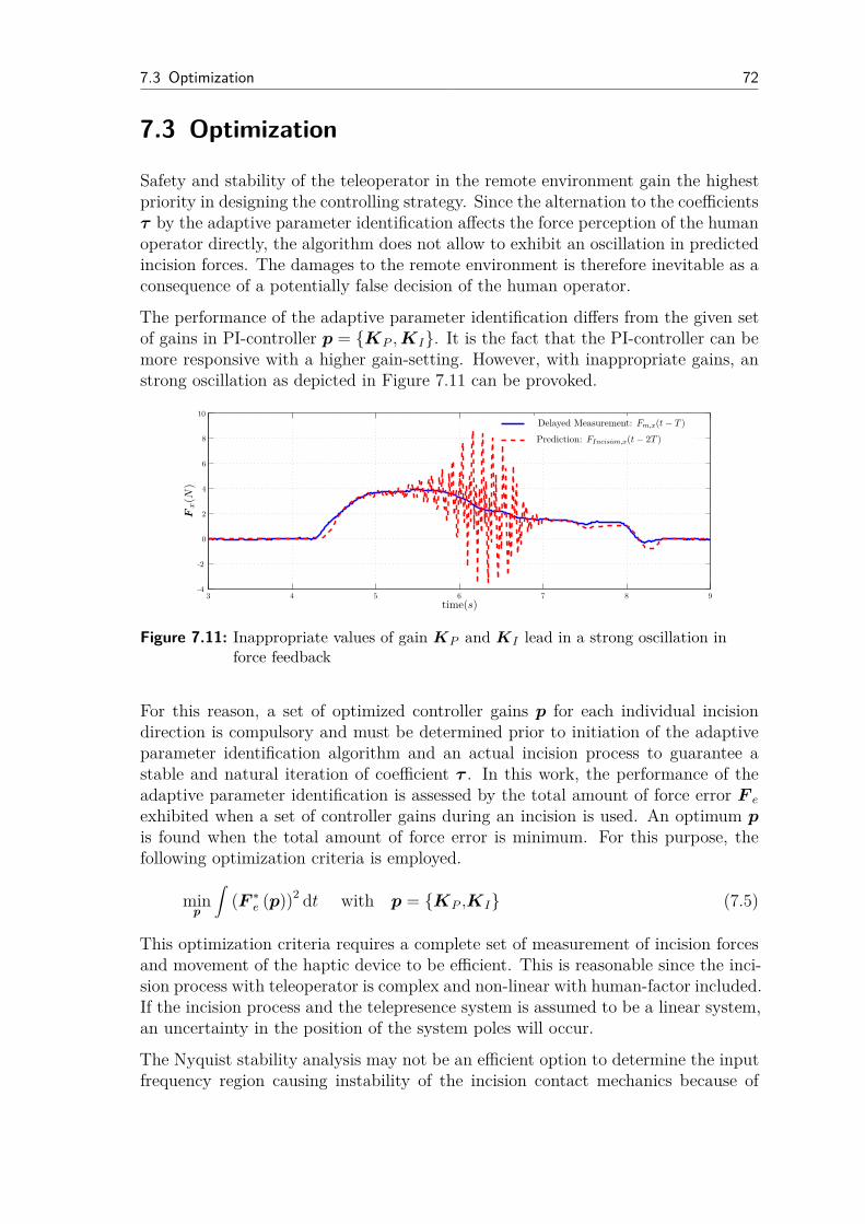
7.3 Optimization 72
7.3 Optimization
Safety and stability of the teleoperator in the remote environment gain the highestpriority in designing the controlling strategy. Since the alternation to the coefficientsτ by the adaptive parameter identification affects the force perception of the humanoperator directly, the algorithm does not allow to exhibit an oscillation in predictedincision forces. The damages to the remote environment is therefore inevitable as aconsequence of a potentially false decision of the human operator.
The performance of the adaptive parameter identification differs from the given setof gains in PI-controller p = KP ,KI. It is the fact that the PI-controller can bemore responsive with a higher gain-setting. However, with inappropriate gains, anstrong oscillation as depicted in Figure 7.11 can be provoked.
3 4 5 6 7 8 9-4
-2
0
2
4
6
8
10
Fx(N
)
time(s)
Delayed Measurement: Fm,x(t− T )
Prediction: FIncision,x(t− 2T )
Figure 7.11: Inappropriate values of gain KP and KI lead in a strong oscillation inforce feedback
For this reason, a set of optimized controller gains p for each individual incisiondirection is compulsory and must be determined prior to initiation of the adaptiveparameter identification algorithm and an actual incision process to guarantee astable and natural iteration of coefficient τ . In this work, the performance of theadaptive parameter identification is assessed by the total amount of force error F e
exhibited when a set of controller gains during an incision is used. An optimum p
is found when the total amount of force error is minimum. For this purpose, thefollowing optimization criteria is employed.
minp
∫
(F ∗
e (p))2 dt with p = KP ,KI (7.5)
This optimization criteria requires a complete set of measurement of incision forcesand movement of the haptic device to be efficient. This is reasonable since the inci-sion process with teleoperator is complex and non-linear with human-factor included.If the incision process and the telepresence system is assumed to be a linear system,an uncertainty in the position of the system poles will occur.
The Nyquist stability analysis may not be an efficient option to determine the inputfrequency region causing instability of the incision contact mechanics because of

7.4 Implementation of the adaptive contact model 73
model parameter uncertainty [38]. Hence, if only a fragment of the measurement isconsidered, a classical controller gain selection based on stable pole placement maylead to an certain set of p which is not suitable for a specific range of frequency ofinput similar as depicted in figure 7.11.
However, the determination of the controller gains can be done off-line using the mea-surement collecting from an incision process with the telepresence system. Moreover,it is found from the experiments that the optimization algorithm is not frequentlyrequired for similar material of test objects. The set of optimum controller gainsprovide a robust performance for handling the incision process with test objectsmade of silicone of different coefficient τ .
7.4 Implementation of the adaptive contact model
With the adaptive incision force model integrated into the geometry deformationsimulation algorithm introduced earlier chapter, the adaptive contact model for theincision process is completed. The Neumann boundary conditions for FEM andXFEM dynamic geometry deformation simulation will be fulfilled by the calculatedincision force.
The initialization of the adaptive contact model is depicted by algorithm 5. Thedynamic geometry deformation simulation must be initiated depending on the cho-sen simulation approach. Algorithm 1 is for FEM with remeshing and Algorithm 3for XFEM. The initialization of the empirical incision force model requires a set ofcoefficients τ 0 specific for the material of the test object and the geometry of scalpel.To determine the cut-depth, the reference level z0 of the surface of the simulatedsoft body must be given. For the adaptive parameter identification algorithm, a setof optimized control gains Kp and KI is required for instantaneous correction ofthe modeling error in the incision force model.
Algorithm 5: Initialization of the adaptive contact model
Initialization geometry deformation simulation: FEM or XFEMDetermine incision force model:
τ 0, z0 −→ equation 7.2
Adaptive parameter identification:
optimized KP , KI
Simulation step indicator:
tn = 0←− n = 0
The adaptive contact model is implemented as depicted in algorithm 6. The scalpelposition is obtained as usual from the employed haptic device. The geometry of
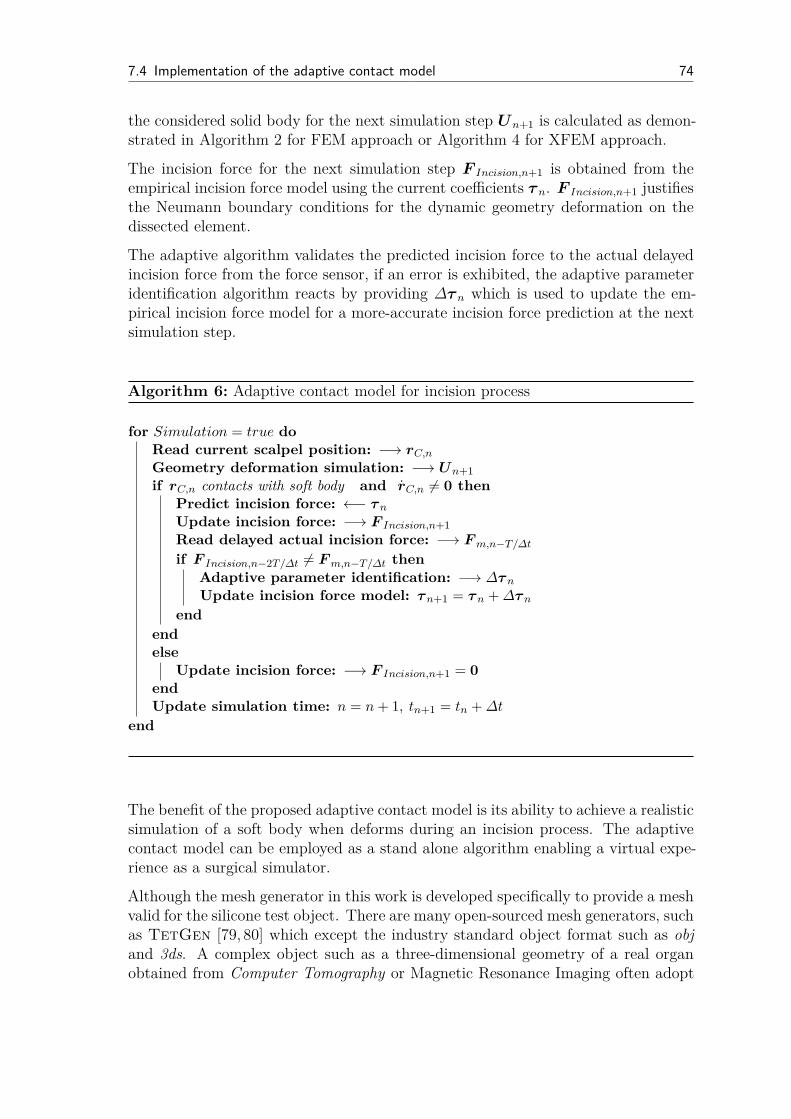
7.4 Implementation of the adaptive contact model 74
the considered solid body for the next simulation step Un+1 is calculated as demon-strated in Algorithm 2 for FEM approach or Algorithm 4 for XFEM approach.
The incision force for the next simulation step F Incision,n+1 is obtained from theempirical incision force model using the current coefficients τ n. F Incision,n+1 justifiesthe Neumann boundary conditions for the dynamic geometry deformation on thedissected element.
The adaptive algorithm validates the predicted incision force to the actual delayedincision force from the force sensor, if an error is exhibited, the adaptive parameteridentification algorithm reacts by providing ∆τ n which is used to update the em-pirical incision force model for a more-accurate incision force prediction at the nextsimulation step.
Algorithm 6: Adaptive contact model for incision process
for Simulation = true do
Read current scalpel position: −→ rC,n
Geometry deformation simulation: −→ Un+1
if rC,n contacts with soft body and rC,n 6= 0 then
Predict incision force: ←− τn
Update incision force: −→ F Incision,n+1
Read delayed actual incision force: −→ Fm,n−T/∆t
if F Incision,n−2T/∆t 6= Fm,n−T/∆t then
Adaptive parameter identification: −→ ∆τn
Update incision force model: τn+1 = τn +∆τn
end
end
else
Update incision force: −→ F Incision,n+1 = 0
end
Update simulation time: n = n+ 1, tn+1 = tn +∆t
end
The benefit of the proposed adaptive contact model is its ability to achieve a realisticsimulation of a soft body when deforms during an incision process. The adaptivecontact model can be employed as a stand alone algorithm enabling a virtual expe-rience as a surgical simulator.
Although the mesh generator in this work is developed specifically to provide a meshvalid for the silicone test object. There are many open-sourced mesh generators, suchas TetGen [79, 80] which except the industry standard object format such as obj
and 3ds. A complex object such as a three-dimensional geometry of a real organobtained from Computer Tomography or Magnetic Resonance Imaging often adopt
7.4 Implementation of the adaptive contact model 75
this formats. Therefore, the contact model in this work can be employed to simulatethe deformation of these objects subjecting to an medical incision.
The reference level of the surface z0 is treated as a constant in this work. This short-coming can be solved with an array of sensor. In the actual teleoperation, a camerasystem is often available. The use of image processing technique can provide thelevel of the surface of where the incision is about to take place. Another possibilityis to use a distance sensor to measure the actual surface level. These practical canenhance the practicality of the adaptive contact model in this work.
Moreover, the adaptive contact model is expandable to include the other discontinu-ities of interest without a complete revision. This is possible since XFEM approachis implemented in the contact model. The discontinuity approximation terms canbe added locally to each affected elements.

8 Experiments and results
This chapter begins with the discussion on the experiments employing the adaptivecontact model developed from chapter 3 to 7. At first, the experimental telepresencesystem and the remote environment will be discussed in section 8.1. Second, insection 8.2, the experiments on an instability from a large time delay during incisionprocesses will be investigated. In this section, the adaptive contact model developedin this work will be demonstrate to compensate the time delay while improve thestability of the telepresence system during incision.
8.1 Experimental telepresence system
The telepresence system employed in this work is depicted in Figure 8.1. The systemcomprises with two essential elements, which are the teleoperator in the remoteenvironment and the local station used by the human operator to manipulate theteleoperator.
1
4
2
3
1. 6-DoF modular robot2. Force-torque sensor with scalpel
3. Test object4. Tension platform
Figure 8.1: Experimental telepresence system
The teleoperator employed in this work is set up in a standard 6-DoF industrialrobot configuration. This configuration is chosen for its adequate work space and
76
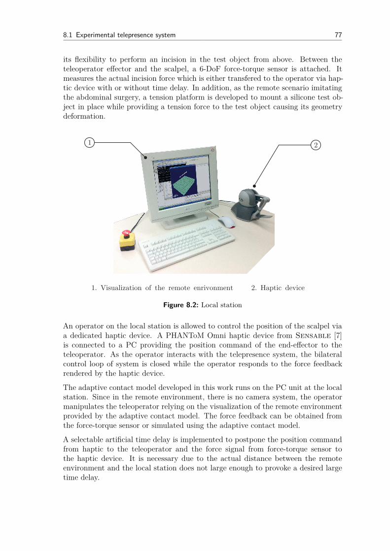
8.1 Experimental telepresence system 77
its flexibility to perform an incision in the test object from above. Between theteleoperator effector and the scalpel, a 6-DoF force-torque sensor is attached. Itmeasures the actual incision force which is either transfered to the operator via hap-tic device with or without time delay. In addition, as the remote scenario imitatingthe abdominal surgery, a tension platform is developed to mount a silicone test ob-ject in place while providing a tension force to the test object causing its geometrydeformation.
2
1. Visualization of the remote enrivonment 2. Haptic device
1
Figure 8.2: Local station
An operator on the local station is allowed to control the position of the scalpel viaa dedicated haptic device. A PHANToM Omni haptic device from Sensable [7]is connected to a PC providing the position command of the end-effector to theteleoperator. As the operator interacts with the telepresence system, the bilateralcontrol loop of system is closed while the operator responds to the force feedbackrendered by the haptic device.
The adaptive contact model developed in this work runs on the PC unit at the localstation. Since in the remote environment, there is no camera system, the operatormanipulates the teleoperator relying on the visualization of the remote environmentprovided by the adaptive contact model. The force feedback can be obtained fromthe force-torque sensor or simulated using the adaptive contact model.
A selectable artificial time delay is implemented to postpone the position commandfrom haptic to the teleoperator and the force signal from force-torque sensor tothe haptic device. It is necessary due to the actual distance between the remoteenvironment and the local station does not large enough to provoke a desired largetime delay.
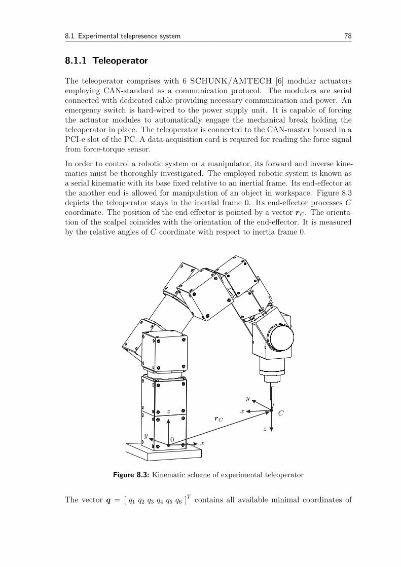
8.1 Experimental telepresence system 78
8.1.1 Teleoperator
The teleoperator comprises with 6 SCHUNK/AMTECH [6] modular actuatorsemploying CAN-standard as a communication protocol. The modulars are serialconnected with dedicated cable providing necessary communication and power. Anemergency switch is hard-wired to the power supply unit. It is capable of forcingthe actuator modules to automatically engage the mechanical break holding theteleoperator in place. The teleoperator is connected to the CAN-master housed in aPCI-e slot of the PC. A data-acquisition card is required for reading the force signalfrom force-torque sensor.
In order to control a robotic system or a manipulator, its forward and inverse kine-matics must be thoroughly investigated. The employed robotic system is known asa serial kinematic with its base fixed relative to an inertial frame. Its end-effector atthe another end is allowed for manipulation of an object in workspace. Figure 8.3depicts the teleoperator stays in the inertial frame 0. Its end-effector processes Ccoordinate. The position of the end-effector is pointed by a vector rC . The orienta-tion of the scalpel coincides with the orientation of the end-effector. It is measuredby the relative angles of C coordinate with respect to inertia frame 0.
x
x
y
yz
z
0
CrC
Figure 8.3: Kinematic scheme of experimental teleoperator
The vector q = [ q1 q2 q3 q4 q5 q6 ]T contains all available minimal coordinates of
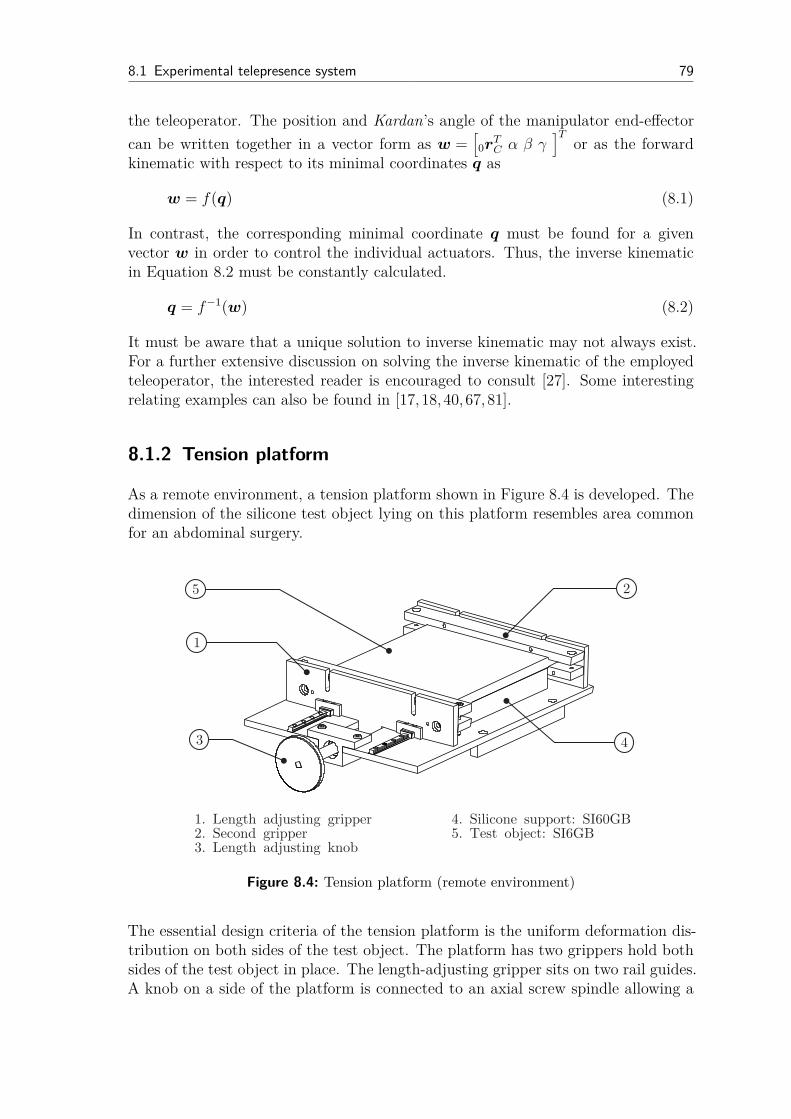
8.1 Experimental telepresence system 79
the teleoperator. The position and Kardan’s angle of the manipulator end-effector
can be written together in a vector form as w =[
0rTC α β γ
]Tor as the forward
kinematic with respect to its minimal coordinates q as
w = f(q) (8.1)
In contrast, the corresponding minimal coordinate q must be found for a givenvector w in order to control the individual actuators. Thus, the inverse kinematicin Equation 8.2 must be constantly calculated.
q = f−1(w) (8.2)
It must be aware that a unique solution to inverse kinematic may not always exist.For a further extensive discussion on solving the inverse kinematic of the employedteleoperator, the interested reader is encouraged to consult [27]. Some interestingrelating examples can also be found in [17,18,40,67,81].
8.1.2 Tension platform
As a remote environment, a tension platform shown in Figure 8.4 is developed. Thedimension of the silicone test object lying on this platform resembles area commonfor an abdominal surgery.
1
3
25
1. Length adjusting gripper2. Second gripper3. Length adjusting knob
4. Silicone support: SI60GB5. Test object: SI6GB
4
Figure 8.4: Tension platform (remote environment)
The essential design criteria of the tension platform is the uniform deformation dis-tribution on both sides of the test object. The platform has two grippers hold bothsides of the test object in place. The length-adjusting gripper sits on two rail guides.A knob on a side of the platform is connected to an axial screw spindle allowing a
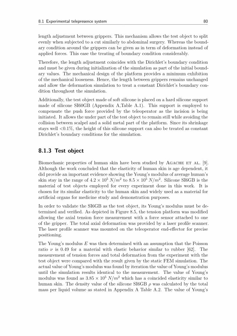
8.1 Experimental telepresence system 80
length adjustment between grippers. This mechanism allows the test object to splitevenly when subjected to a cut similarly to abdominal surgery. Whereas the bound-ary condition around the grippers can be given as in term of deformation instead ofapplied forces. This ease the treating of boundary condition considerably.
Therefore, the length adjustment coincides with the Dirichlet’s boundary conditionand must be given during initialization of the simulation as part of the initial bound-ary values. The mechanical design of the platform provides a minimum exhibitionof the mechanical looseness. Hence, the length between grippers remains unchangedand allow the deformation simulation to treat a constant Dirichlet’s boundary con-dition throughout the simulation.
Additionally, the test object made of soft silicone is placed on a hard silicone supportmade of silicone SI60GB (Appendix A,Table A.1). This support is employed tocompensate the push force provided by the teleoperator as the incision is beinginitiated. It allows the under part of the test object to remain still while avoiding thecollision between scalpel and a solid metal part of the platform. Since its shrinkagestays well <0.1%, the height of this silicone support can also be treated as constantDirichlet’s boundary conditions for the simulation.
8.1.3 Test object
Biomechanic properties of human skin have been studied by Agache et al. [9].Although the work concluded that the elasticity of human skin is age dependent, itdid provide an important evidence showing the Young’s modulus of average human’sskin stay in the range of 4.2× 10⁵ N/m2 to 8.5× 10⁵ N/m2. Silicone SI6GB is thematerial of test objects employed for every experiment done in this work. It ischosen for its similar elasticity to the human skin and widely used as a material forartificial organs for medicine study and demonstration purposes.
In order to validate the SI6GB as the test object, its Young’s modulus must be de-termined and verified. As depicted in Figure 8.5, the tension platform was modifiedallowing the axial tension force measurement with a force sensor attached to oneof the gripper. The total axial deformation was provided by a laser profile scanner.The laser profile scanner was mounted on the teleoperator end-effector for precisepositioning.
The Young’s modulus E was then determined with an assumption that the Poissonratio ν is 0.49 for a material with elastic behavior similar to rubber [62]. Themeasurement of tension forces and total deformation from the experiment with thetest object were compared with the result given by the static FEM simulation. Theactual value of Young’s modulus was found by iteration the value of Young’s modulusuntil the simulation results identical to the measurement. The value of Young’smodulus was found as 3.85 × 10⁵ N/m2 which has a coincided elasticity similar tohuman skin. The density value of the silicone SI6GB ρ was calculated by the totalmass per liquid volume as stated in Appendix A Table A.2. The value of Young’s
8.1 Experimental telepresence system 81
1
2
3
1. Laser profile scanner2. Axial force sensor
3. Test object: SI6GB
Figure 8.5: Verification of Young’s modulus of experimental silicone
modulus E, Poisson ration ν and material density ρ can be used for simulation withFEM and XFEM as material parameters.
8.1.4 Software framework
The software development in this work is multi-thread coding. In computer science,the term threaded code refers to a compiler implementation technique where thegenerated code essentially consists entirely of calls to subroutines. The code maybe processed by an interpreter, or may simply be a sequence of machine code callinstructions. One of the main advantages of threaded code is that it is very com-pact, compared to code generated by alternative code generation techniques andalternative calling conventions. This enables programmers to concentrate mostly onthe structure of the software framework and synchronization mechanism betweensubroutines and program modules.
Windows XP 32-bit is employed as the operating system and developing environ-ment of the software package in this works. This operating system is not a real-timeoperating system which the exact execution time of a command can not be given.However, it allows multi-threading and ability to set the priority of each executableprogram modules. Thus, the software framework was developed by considering a

8.2 Time delay compensation utilizing contact model 82
proper hierarchy of the program modules priority. The software framework com-prises with 3 important program modules
1. Geometry deformation simulation and visualization
2. Haptic interface and Adaptive empirical incision force algorithm
3. Central teleoperator kinematic control
The haptic interface gains the highest priority due to its demanding a high-samplingrate of force feedback generated by the adaptive empirical incision force algorithm.The central teleoperator kinematic control has the second highest priority, since asmooth movement of the telerobot can be achieved by updating the position com-mand at lower sampling of 100Hz. This is possible because the actuator moduleshave cascade controller built-in and responsible of the path generation at the mini-mal coordinate level. The geometry deformation simulation with the sampling rateof visualization as low as 30Hz is sufficient while the animation remains seamless.Therefore, it is given the lowest priority. An open-source software package CHAI3Dwhich is well-known for haptic applications [24] is employed to associate the devel-opment of this software framework. This software package provides a unified hapticinterface to some of widely accepted haptic devices available. Its visualization isimplemented based on standard OpenGL API [4]. Although the haptic feedbackrendering is also extensively available by the package, it does not have incision forcerendering capability. Therefore, the incision force calculation is done solely relyingon the implementation proposed in this work.
8.2 Time delay compensation utilizing contactmodel
The analysis of the effect of time delay is essential for the utmost understandingof the instabilities during a telepresence operation. The typical linear evaluationmethods based on root locus and bode diagram are not a proper investigation toolto determine the instability during an actual medical incision due to the complexityof modeling and non-linearity of the incision contact mechanics. For a comparisonpurpose, a large time delay causes reduction in gain-margin and phase-margin froma linear control theory. Instead, the investigation and discussions of the impact oftime delay in this section was done based on three experiments.
Section 8.2.1 comprises with two experiments which are designed to address theissues of time delay during incision process with a telepresence system. In Sec-tion 8.2.2, with the third experiment, the utilization of adaptive contact modeldeveloped in this work will be discussed as a solution to the time delay problem.
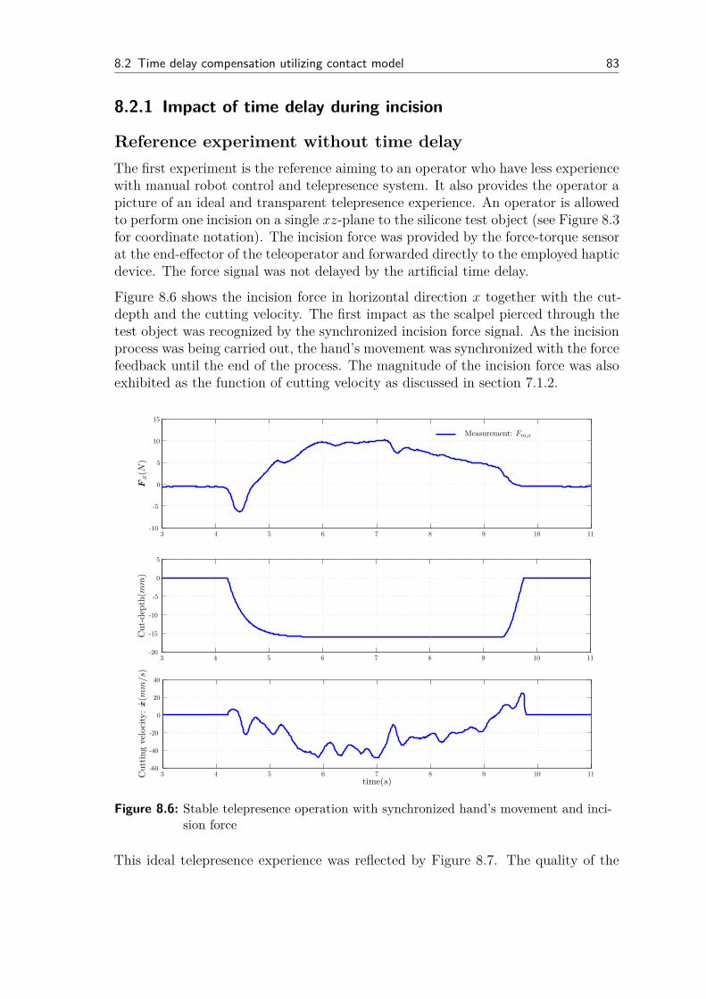
8.2 Time delay compensation utilizing contact model 83
8.2.1 Impact of time delay during incision
Reference experiment without time delay
The first experiment is the reference aiming to an operator who have less experiencewith manual robot control and telepresence system. It also provides the operator apicture of an ideal and transparent telepresence experience. An operator is allowedto perform one incision on a single xz-plane to the silicone test object (see Figure 8.3for coordinate notation). The incision force was provided by the force-torque sensorat the end-effector of the teleoperator and forwarded directly to the employed hapticdevice. The force signal was not delayed by the artificial time delay.
Figure 8.6 shows the incision force in horizontal direction x together with the cut-depth and the cutting velocity. The first impact as the scalpel pierced through thetest object was recognized by the synchronized incision force signal. As the incisionprocess was being carried out, the hand’s movement was synchronized with the forcefeedback until the end of the process. The magnitude of the incision force was alsoexhibited as the function of cutting velocity as discussed in section 7.1.2.
3 4 5 6 7 8 9 10 11-10
-5
0
5
10
15
3 4 5 6 7 8 9 10 11-20
-15
-10
-5
0
5
3 4 5 6 7 8 9 10 11-60
-40
-20
0
20
40
Fx(N
)
time(s)
Cut
-dep
th(mm
)C
utti
ngve
loci
ty:x
(mm/s)
Measurement: Fm,x
Figure 8.6: Stable telepresence operation with synchronized hand’s movement and inci-sion force
This ideal telepresence experience was reflected by Figure 8.7. The quality of the
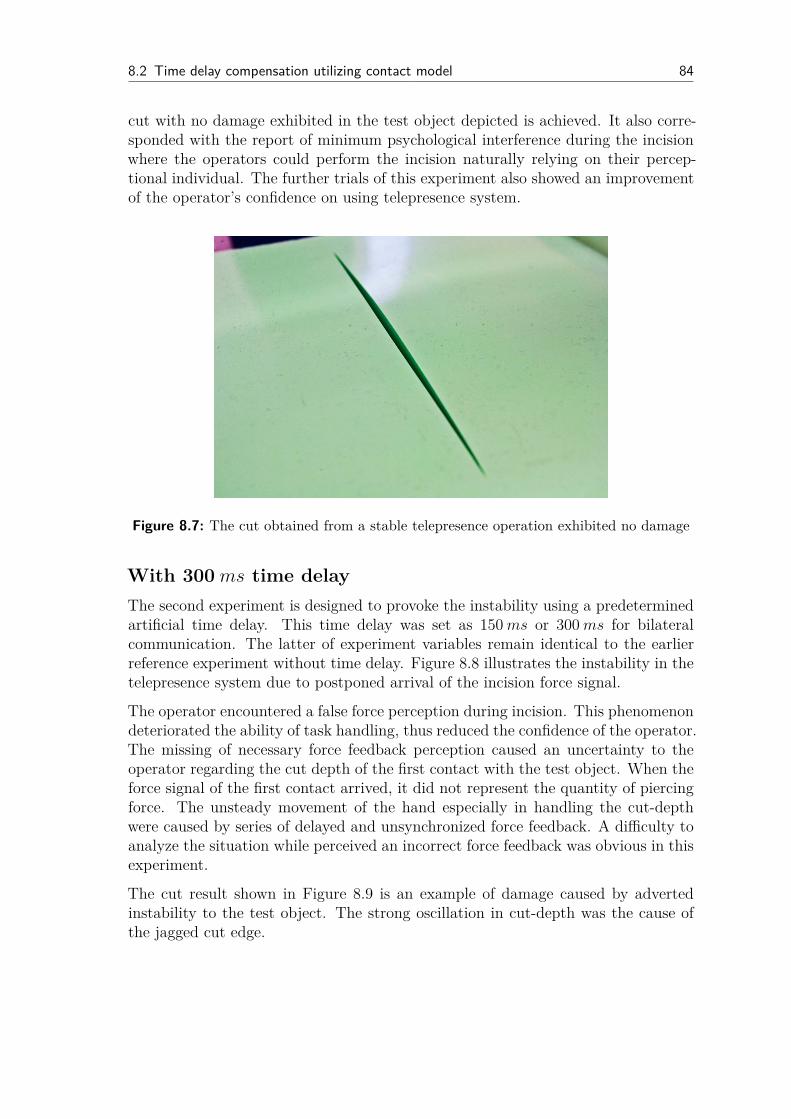
8.2 Time delay compensation utilizing contact model 84
cut with no damage exhibited in the test object depicted is achieved. It also corre-sponded with the report of minimum psychological interference during the incisionwhere the operators could perform the incision naturally relying on their percep-tional individual. The further trials of this experiment also showed an improvementof the operator’s confidence on using telepresence system.
Figure 8.7: The cut obtained from a stable telepresence operation exhibited no damage
With 300 ms time delay
The second experiment is designed to provoke the instability using a predeterminedartificial time delay. This time delay was set as 150ms or 300ms for bilateralcommunication. The latter of experiment variables remain identical to the earlierreference experiment without time delay. Figure 8.8 illustrates the instability in thetelepresence system due to postponed arrival of the incision force signal.
The operator encountered a false force perception during incision. This phenomenondeteriorated the ability of task handling, thus reduced the confidence of the operator.The missing of necessary force feedback perception caused an uncertainty to theoperator regarding the cut depth of the first contact with the test object. When theforce signal of the first contact arrived, it did not represent the quantity of piercingforce. The unsteady movement of the hand especially in handling the cut-depthwere caused by series of delayed and unsynchronized force feedback. A difficulty toanalyze the situation while perceived an incorrect force feedback was obvious in thisexperiment.
The cut result shown in Figure 8.9 is an example of damage caused by advertedinstability to the test object. The strong oscillation in cut-depth was the cause ofthe jagged cut edge.

8.2 Time delay compensation utilizing contact model 85
8 9 10 11 12 13 14 15 16 17 18 19 20
0
5
10
15
8 9 10 11 12 13 14 15 16 17 18 19 20-20
-15
-10
-5
0
5
8 9 10 11 12 13 14 15 16 17 18 19 20-100
-50
0
50
100
Fx(N
)
time(s)
Cut
-dep
th(mm
)C
utti
ngve
loci
ty:x
(mm/s
)Delayed measurement: Fm,x
300ms
Figure 8.8: Unstable incision with a strong oscillation in cut-depth due to non-synchronization between hand’s movement and force feedback perception
Damage to test object
Figure 8.9: With 300ms time delay, the instability caused damage to test object pre-senting a jagged cut edge.
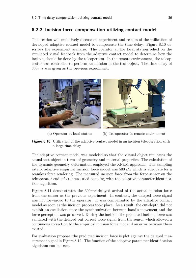
8.2 Time delay compensation utilizing contact model 86
8.2.2 Incision force compensation utilizing contact model
This section will exclusively discuss on experiment and results of the utilization ofdeveloped adaptive contact model to compensate the time delay. Figure 8.10 de-scribes the experiment scenario. The operator at the local station relied on thesimulated visual feedback from the adaptive contact model to determine how theincision should be done by the teleoperator. In the remote environment, the teleop-erator was controlled to perform an incision in the test object. The time delay of300ms was given as the previous experiment.
(a) Operator at local station (b) Teleoperator in remote environment
Figure 8.10: Utilization of the adaptive contact model in an incision teleoperation witha large time delay
The adaptive contact model was modeled so that the virtual object replicates theactual test object in terms of geometry and material properties. The calculation ofthe dynamic geometry deformation employed the XFEM approach. The samplingrate of adaptive empirical incision force model was 500Hz which is adequate for aseamless force rendering. The measured incision force from the force sensor on theteleoperator end-effector was used coupling with the adaptive parameter identifica-tion algorithm.
Figure 8.11 demonstrates the 300ms-delayed arrival of the actual incision forcefrom the sensor as the previous experiment. In contrast, the delayed force signalwas not forwarded to the operator. It was compensated by the adaptive contactmodel as soon as the incision process took place. As a result, the cut-depth did notexhibit an oscillation since the synchronization between hand’s movement and theforce perception was preserved. During the incision, the predicted incision force wasvalidated with the delayed but correct force signal from the sensor which allowed acontinuous correction to the empirical incision force model if an error between themexisted.
For evaluation propose, the predicted incision force is plot against the delayed mea-surement signal in Figure 8.12. The function of the adaptive parameter identificationalgorithm can be seen.

8.2 Time delay compensation utilizing contact model 87
3 4 5 6 7 8-2
0
2
4
6
8
10
12
3 4 5 6 7 8-20
-15
-10
-5
0
5
3 4 5 6 7 8-150
-100
-50
0
50
Fx(N
)
time(s)
Cut
-dep
th(mm
)C
utti
ngve
loci
ty:x
(mm/s
)Adaptive prediction: FIncision,x
Delayed measurement: Fm,x
300ms
Figure 8.11: Adaptive incision force model provides an accurate and stable telepresenceoperation during an incision
3 4 5 6 7 8-2
0
2
4
6
8
10
12
3 4 5 6 7 8-4
-3
-2
-1
0
1
2
3
4
Fx(N
)F
∗ e,x(N
)
time(s)
Delayed Measurement: Fm,x
Adaptive Prediction: FIncision,x(t− 2T )
Figure 8.12: Accuracy improvement in incision force error F ∗e,x with adaptive parameter
identification algorithm

8.2 Time delay compensation utilizing contact model 88
The algorithm acknowledged 300ms after the incision began that the incision forcemodel was not correct with a large amount force error F ∗
e,x. The algorithm respondedby adjusting the coefficient τx in the empirical incision force model allowing F ∗
e,x
to decline as the incision was carried out without an interruption. The proposedalgorithm was successfully predicted an incision force without significant delayed.It provided a transparent correction during the actual incision was taken place.As a result, a stable and comparable realistic telepresence operation was obtained.Figure 8.13 illustrates the cut in the test object which does not exhibit the damagedue to existing large time delay compared to Figure 8.9. On the other hand, asimilar result found in 8.7 by the reference experiment was instead achieved.
Figure 8.13: Adaptive contact model maintains the stability with a result similar tofigure 8.7
Although it is not a focus of this work to interpret the success rate of the teleop-eration with a psychological assessment, it is necessary to discuss that the resultspresented in this chapter subject to the human-factor of the operators. Therefore,the results from each experiment should be relatively evaluated with the results fromthat particular operator and not from the others.
In the second experiment, where the 300ms was given, the better results wereobserved from operators with an understanding of telepresence and time delay. Thisgroup of operators provided a certain level of extra force reducing the eradicatemovement of the haptic device. Therefore, the delayed force feedback in this casewere neglected as a perception but treated as an interference instead. Since it was notconstrained how the operators should make an incision, some operators moved theirhands slowly enough to obtain a reasonable level of synchronization even thoughthe force signal was delayed severely. The time delay was therefore not a significantissue in this case. These individual abilities of handling a machine control interfacedepend on personal experiences which result in different levels of success and qualityof the achievements.
8.2 Time delay compensation utilizing contact model 89
It is arguable that some telepresence operations may be successful carried out with-out a force perception. Specifically, when the force is distorted, such as from timedelay. However, this may not be correct for a medical teleoperation. The demandof an accurate force feedback especially for a surgical teleoperation was studied byWagner et al. [97]. It is discussed that the force feedback does not only improvethe rate of success significantly in a medical task handling but more importantlyprevent a damage to the scenery. Morris et al. presented an evidence of ben-efits of a task training gained from a combination of visual and haptic [59]. Thework finds that a visuohaptic training is significantly more accurate than a visualor haptic training alone.
From discussions during the experiments in this work, it can be concluded with con-fidence that a correct, or quantitatively speaking, realistic telepresence experience isalways preferred. An intuitive telepresence experience proves to help operators to ad-just themselves faster to telepresence control interface while allowing their personalskills to be expressed naturally and with confident. The utilization of the proposedadaptive contact model fulfills its role by substantially provide the operators withan accurate incision force even the communication channel is subjected to a largetime delay.

9 Conclusion and future works
9.1 Discussion
In this work, the time delay problem in a medical telepresence system specific duringan incision process is addressed. The compensation of time delay with an adaptivecontact model is proposed. The adaptive contact model is developed to simulate adynamic geometry deformation for the visualization of a soft body and the corre-sponding incision force in real-time. The adaptive parameter identification algorithmin the contact model provides an on-line verification capability of the simulated in-cision force during the actual incision in telepresence operation.
The development begins with a thorough analysis of the incision mechanics in termsof continuum mechanics in chapter 3. A discussion is made on the configurationalchanges of material points in a soft body when a cut evolves. It leads to the needof a remapping of the dynamic governing system of equation. To realize a dynamicgeometry deformation simulation, a continuum soft body is discretized into finitenumbers of smaller domains. FEM and XFEM are two approaches investigated inthis work.
In chapter 4, in order to satisfy the remapping of configurational changes due to ma-terial point separation, FEM requires a reconsideration of the spatial discretizationcalled remeshing. It results in an update to the Lagrange mesh at each simulationstep. An example of remeshing is also developed allowing the cut to evolve on theedge of tetrahedron elements. FEM with remeshing can be seen to treat the materialdiscontinuity from the cut in a global domain. Therefore, the governing system ofequations is reassembled after the current topology before the remapped boundaryconditions can be applied.
On the other hand, in chapter 5, XFEM approach uses a shifted function to approx-imate a cut as a material discontinuity to an element. The rest of the elements inthe initial Lagrange mesh remains unchanged. This approach enables the governingsystem of equation to expand systematically without the initial governing system ofequations to be completely rearranged.
In chapter 6, the discussion on the practicality of FEM and XFEM as a develop-ment tool for a incision contact model is brought. In contrary to FEM, XFEMdemonstrates a good flexibility in handling a dynamic simulation problem with dis-continuities. Therefore, XFEM is evaluated to be more practical and suitable for acontact model for incision simulation.
90

9.2 Outlooks 91
The incision force from the scalpel is a nodal contact force acting on the elementwhich is being cut. The governing system of equations require the incision forceto be given to fulfill the Neumann boundary conditions. Therefore, in chapter 7,an empirical incision force is developed after the friction model. Considering anactual surgical telepresence scenery, a perfect modeling and parameterization of theproposed incision force model can be difficult to achieve. The optimized adaptiveparameter identification algorithm is proposed in this work for a constant verificationof the accuracy of the contact model during the incision in an actual telepresenceoperation. The algorithm proves a substantial improvement in the accuracy whiletransparently provides a correct incision force perception to the human operators.
In contrast to general telepresence systems, the experimental telepresence system isdeveloped to subject to a large time delay (300ms) in communication in chapter 8.This setup purposefully provokes the instability during the actual incision. In anexperiment, the instability is observed from a non-synchronization of the hand’smovement and the force feedback. The operators are subjected to perceive this falsecontact force while penetrates the test object. The experiment shows that insteadthe force feedback provides the human operators a comprehend contact information,it interferences the process. With a scalpel at the end-effector of the teleoperator,the damage occurred to the test object is inevitable.
In another experiment, the time delay is completely compensated from the controlroute of the telepresence system using the predicted visualization and force signalobtained from the adaptive contact model developed in this work. Thus, a stableincision with a telepresence system subjected to a large time delay is achieved.
9.2 Outlooks
The proposed contact model for incision process developed in this work can befurther developed to be an interactive surgical simulator framework similar to theSOFA framework [10]. From the derivations seen in this work, XFEM is a convinc-ing approach for the modeling of a contact mechanics especially with the differenttypes of discontinuities at the same time. The contact library shall be inventedto support an implementation of a contact model with a comprehensive archive ofmodel and biomechanical properties of different organs can be obtained similar tothe work of Agache et al. [9], Schillhuber [71] and Zhao [100].
Three-dimensional geometry of patient’s organs can nowadays easily obtained fromconventional Computerized Tomography (CT), Magnetic Resonance Imaging (MRI)techniques. It can be combined with the mechanical properties supplied by thecontact library to develop an approximate contact model of a patient. This contactmodel with realistic visual graphic and haptic interaction can provide an intensifiedtraining of medical residents and doctors which induces failure prevention and amore efficient surgical operation.
9.2 Outlooks 92
Telepresence technology is a widely embraced application. In medical fields, thetelesurgery has been proving and slowly accepted for its potential as a better optionto the patient. However, before this goal can be accomplished, some technicallimitations such as a successful skill transfer between a doctor and a robotic systemmust be realized. This can depend on a flawless feedback perception provided by therobotic system to the surgeon. The adaptive contact model developed in this workproved to provide an accurate incision force. However, this can be achieved becausethe experiment scenery such as the position of the test object does not change. Inan actual surgery, the contact model can encounter a difficulty of the treatment ofthe boundary conditions. This problem can be solved by using a camera system tocalculate the positions of the object of interest while constantly update the Dirichletboundary conditions in the simulation.
The experiments in this work did not involve in an psychological assessment. Theresults conclude that the accurate incision force is preferred. Nevertheless, since thehuman factor or preference to the interaction with the robot control interface canbe varied, a systematic evaluation considering human preference with the rate ofsuccess can provide a new information for the improvement of the contact modeland the control strategy of the telepresence system.
Within Collaborative Research Centre 453, it has been discussed of the integrationof the various methods to provide a stable telepresence system in different purposes.The combination of the proposed adaptive contact model with the transparent datareduction [43] and data compression in communication [88] is a logical approach. Thecontact model can supplement the simulation results in cases the data is completelylost. Therefore, the teleoperation can be carried out without an interruption.
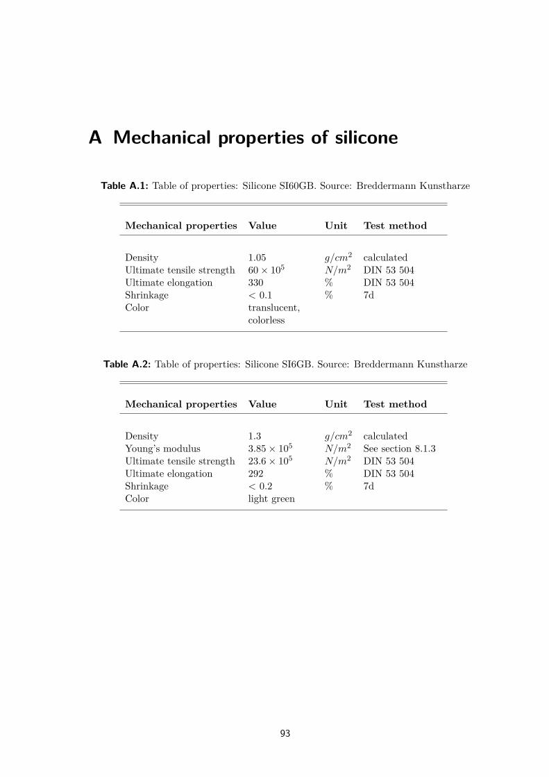
A Mechanical properties of silicone
Table A.1: Table of properties: Silicone SI60GB. Source: Breddermann Kunstharze
Mechanical properties Value Unit Test method
Density 1.05 g/cm2 calculatedUltimate tensile strength 60× 105 N/m2 DIN 53 504Ultimate elongation 330 % DIN 53 504Shrinkage < 0.1 % 7dColor translucent,
colorless
Table A.2: Table of properties: Silicone SI6GB. Source: Breddermann Kunstharze
Mechanical properties Value Unit Test method
Density 1.3 g/cm2 calculatedYoung’s modulus 3.85× 10⁵ N/m2 See section 8.1.3Ultimate tensile strength 23.6× 10⁵ N/m2 DIN 53 504Ultimate elongation 292 % DIN 53 504Shrinkage < 0.2 % 7dColor light green
93
Bibliography
[1] Sonderforschungsbereich 453 (SFB 453). Website.http://www.lrz.de/~t8241ad/webserver/webdata/index.html
[2] Khronos Group - Open Standard for Parallel Programming of HeterogeneousSystems : OpenCL. Website. www.khronos.org/opencl/. Version: 2011
[3] Nvidia Technology - Compute Unified Device Architecture : CUDA. Website.www.nvidia.com. Version: 2011
[4] Open Graphics Library: OpenGL. Website. www.opengl.org. Version: 2011
[5] Open Multi-Processing : OpenMP. Website. www.openmp.org. Version: 2011
[6] SCHUNK GmbH & Co. KG. Website. www.opengl.org. Version: 2011
[7] Sensable Technologies. Website. www.sensable.com. Version: 2011
[8] Abe, N. ; Yamanaka, K.: Smith predictor control and internal model control - atutorial. In: SICE 2003 Annual Conference vol. 2, 2003, pp. 1383–1387
[9] Agache, P.G. ; Monneur, C. ; Leveque, J. L. ; Rigal, J. D.: MechanicalProperties and Young’s Modulus of Human Skin in Vivo. In: Archives ofDermatological Research 269 (1980), pp. 221–232
[10] Allard, J. ; Cotin, S. ; Faure, F. ; Bensoussan, P. ; Poyer, F. ; Duriez, C.; Delingette, H. ; Jeřábková, L. G.: SOFA - an Open Source Framework forMedical Simulation. In: Medecine Meets Virtual Reality (2007), pp. 13–18
[11] Armstrong-Hélouvry, B. ; Dupont, P. ; Wit, C. C.: A Survey of Models,Analysis Tools and Compensation Methods for the Control of Machines withFriction. In: Automatica 30 (1994), pp. 1083–1138
[12] Ashrafiuon, H.: Design Optimization of Aircraft Engine-Mount Systems. In:Vibration and Control of Mechanical Systems 61 (1993), pp. 117–131
[13] ch. Efficient algorithms for layer assignment problems. In: Bathe, K.-J:Finite-Elemente-Methoden. San Francisco, CA : Freeman, 1973, pp. 63–83
[14] Belytschko, T. ; Black, T.: Elastic Crack Growth in Finite Elements WithMinimal Remeshing. In: International Journal for Numerical Methods inEngineering 45 (1999), pp. 601–620
[15] Belytschko, T. ; Liu, W. K. ; Moran, B.: Nonlinear Finite Elements forContinua and Stuctures. John Wiley & Sons, Inc., 2000
[16] Bordas, Ss ; Legay, A. ; Gravouil, A.: X-FEM Mini-Course. 2007. –Lecture note from EPSFL short-course
94
Bibliography 95
[17] Bremer, H. ; Pfeiffer, F.: Dynamik und Regelung mechanischer Systeme.Teuber Verlag, 1988
[18] Bremer, H. ; Pfeiffer, F.: Elastische Mehrkörpersysteme. Teuber Verlag, 1992
[19] Bruyns, C. D. ; Montgomery, K.: Generalized Interactiions Using VirtualTools within the Spring Framework: Cutting. In: Medicine Meets Virtual Reality02/10 (2002), pp. 79–85
[20] Burnett, D. S.: Finite Element Analysis. Addison-Wesley, 1987
[21] Chessa, J. ; Belytschko, T.: An enriched finite element method and level setsfor axisymmetric two-phase flow with surface tension. In: International Journalfor Numerical Methods in Engineering 58 (2003), pp. 2041–2064
[22] Clarke, S. ; Schillhuber, G. ; Zaeh, M. F. ; Ulbrich, H.: The Effect ofSimulated Inertia and Force Prediction on Delayed Telepresence. In: Presence:Teleoperators and Virtual Environments 16 (2007), October, nr. 5, pp. 543–558. –Special Topic: Teleoperators and Virtual Environments
[23] Clough, R. ; Penzien, J. ; Edition 2nd (ed.): Dynamics of Structures.MeGraw-Hill, 1993
[24] Conti, F. ; Barbagli, F. ; Morris, D. ; Sewell, C.: CHAI 3D - AnOpen-Source Library for the Rapid Development of Haptic Scenes. In: IEEEWorld Haptics, 2005
[25] Dolbow, J.: An Extended Finite Element Method with DiscontinuousEnrichment for Applied Mechanics, Northwestern University, Evanston, IL, Diss.,1999
[26] Eberhard, P.: Kontaktuntersuchungen durch hybride Mehrkörpersystem / FiniteElemente Simulationen. Shaker Verlag, 2000
[27] Engelke, R.: Modellierung und Optimierung von Robotern mit einseitigenBindungen und lokalen Verspannungen. München, Germany, TechnischeUniversität München, Fakultät für Maschinenewesen, Diss., 2008
[28] Fite, K.B. ; Goldfarb, M. ; Rubio, A.: Transparent telemanipulation in thepresence of time delay. In: Advanced Intelligent Mechatronics, 2003. AIM 2003.Proceedings. 2003 IEEE/ASME International Conference on vol. 1, 2003, pp. 254– 259 vol.1
[29] Fries, T. P. ; Belytschko, T.: The Instrinsic XFEM: A Method for ArbitraryDiscontinuities Without Additional Unknowns. In: International Journal forNumerical Methods in Engineering 68 (2006), pp. 1358–1385
[30] Fuller, D. D.: Theory and practice of lubrication for engineers. In: Journal ofSynthetic Lubrication 1, pp. 314
[31] Goangseup, Z. ; Belytschko, T.: New Crack-Tip Elements for XFEM andApplications to Cohesive Cracks. In: International Journal for NumericalMethods in Engineering 57 (2003), pp. 2221–2240

Bibliography 96
[32] Golle, A. ; Ulbrich, H.: Contact Models for Real-Time-Simulation inTelepresence Applications. In: Inproceeding of EuroHaptics 2004, 2004, pp.381–384
[33] Golle, A. ; Ulbrich, H. ; Pfeiffer, F.: Real-time simulation of non-smoothcontacts in telepresence. In: Industrial Technology, 2003 IEEE InternationalConference on, 2003 (2), pp. 675–679
[34] Green, P. S. ; Hill, J. W. ; Jensen, J. F. ; Shah, A.: Telepresence Surgery. In:IEEE Engineering in Medicine and Biology 14 (1995), pp. 324–329
[35] Groß, S. ; Reusken, A.: An extended pressure finite element space for two-phase incompressible flows with surface tension. In: Journal of ComputationalPhysics 224 (2007), pp. 40–58
[36] Gürses, E. ; Miehe, C.: A Computational Framework of Three-DimensionalConfigurational-Force-Driven Brittle Crack Propagation. In: Computer methodsin applied mechanics and engineering (2008)
[37] Hahn, C.: Models, Algorithms and Software Concepts for Contact andFragmentation in Computational Solid Mechanics, Faculty of Civil Engineering,Universität Hannover, Diss., 2005
[38] Hahn, J. ; Edison, T. ; Edgar, T. F.: A Note on Stability Analysis Using BodePlots. In: ChE classroom (2001)
[39] Hansbo, A. ; Hansbo, P.: A Finite Element Method for the Simulation ofStrong and Weak Discontinuities in Solid Mechanics. In: Computer methods inapplied mechanics and engineering 193 (2004), pp. 3523 – 3540
[40] Heimann, B. ; Gerth, W. ; Popp, K.: Mechatronik: Komponent - Methoden -Beispiele. 2. Fachbuchverlag Leipzig, 2000
[41] ch. 14. In: Held, R. ; Durlach, N.l: TELEPRESENCE, TIME DELAY, ANDADAPTATION. Taylor and Francis, 1991, pp. 232–246
[42] Hirche, S. ; Bauer, A. ; Buss, M.: Transparency of Haptic TelepresenceSystems with Constant Time Delay. In: IEEE Conference on ControlApplications, 2005
[43] Hirsche, S. ; Buss, M.: Transparent Data Reduction in Networked Telepresenceand Teleaction Systems Part II: Time-Delayed Communication. In: Presence:Teleoperators and Virtual Environments 16, No. 5 (2007), pp. 532–542
[44] Hirzinger, G. ; Hagn, U.: Flexible Heart Surgery. In: German Research(Magazine of the German Research Foundation DFG) 1 (2010). – Available online
[45] Hrenikoff, A.: Solution of probelms in eleasticity by the framwork method. In:ASME Journal of Applied Mechanics A8 (1941), pp. 169–175
[46] Jeřábková, L.: Interactive Cutting of Finite Elements based Deformable Objectsin Virtual Environment, Rheinisch-Westfälischen Technischen Hochschule Aachen,Faculty of Mathematics, Computer Science and Natural Sciences, Dissertation,2007
Bibliography 97
[47] Johnston, M. D. ; Rabe, K. J.: Integrated Planning for Telepresence with TimeDelays. In: 2nd IEEE International Conference on Space Mission Challenges forInformation Technology SMCIT06, 2006, pp. 140–146
[48] Knoll, A.: Toward High-Definition Telepresence. In: Presence: Teleoperatorsand Virtual Environments 16 (2007), nr. 5
[49] Kundu, K. ; Olano, Ol: Tissue resection using delayed updates in a tetrahedralmesh. In: Studies in Health Technology and Informatics (2007)
[50] Landzettel, K. ; Preusche, C. ; Albu-Schaffer ; A. Reintsema, D. ;Rebele, D. ; Hirzinger, G.: Robotic On-Orbit Servicing - DLR’s Experienceand Perspective. In: IEEE/RSJ International Conference on Intelligent Robotsand Systems, 2006, pp. 4587
[51] Lang, C. B. ; Pucker, N.: Mathematische Methoden in der Physik. 2.Spektrum Akademischer Verlag
[52] Laursen, T. A. ; Simo, J. C.: A Continuum-Based Finite Element Formulationfor the Implicit Solution of Multibody, Large Deformation-Frictional ContactProblems. In: International Journal for Numerical Methods in Engineering 36(2005), pp. 3451–3485
[53] Mayer, H.: Human Machine Skill Transfer in Robot Assisted, MinimallyInvasive Surgery. Munich, Germany, Technische Universität München, Diss., 2008
[54] McHenry, D.: A lattice analogy for the solution of plane stress problems. In:International Journal of Civil Engineering 21 (1943), pp. 59–82
[55] Mitsuishi, M. ; Iizuka, Y. ; Watanabe, H. ; Hashizume, H. ; Fujiwara, K.:Remote operation of a micro-surgical system. In: IEEE International Conferenceon Robotics and Automation vol. 2, 1998, pp. 1013–1019
[56] Moës, N. ; Dolbow, J. ; Belytschko, T.: A Finite Element Method For CrackGrowth Without Remeshing. In: International Journal for Numerical Methods inEngineering 46 (1999), pp. 131–150
[57] Moës, N. ; Sukumar, N. ; Moran, B. ; Belytschko, T.: An Extended FiniteElement Method (X-FEM) For Two- and Threes-Dimensional Crack Modeling.In: European Congress on Computational Methods in Applied Sciences andEngineering ECCOMAS 2000, 2000
[58] Mohammadi, S.: Extended finite element method for fracture analysis ofstructures. Blackwell Publishing Ltd, 2008
[59] Morris, D. ; Tan, H. ; Barbagli, F. ; Chang, T. ; Salisbury, K.: HapticFeedback Enhances Force Skill LearningŤ, to appear. In: Proceedings of the 2007World Haptics Conference, 2007, pp. 22–24
[60] Newmark, N. M.: Numerical methods of analysis in bars, plates and elasticbodies. In: Numerical Methods in Analysis in Engineering (1949)
[61] Newmark, N. M.: A Method of Computation for Structural Dynamics. In:Journal of Engineering Mechanics Division 85 (1959), pp. 67–94
Bibliography 98
[62] O’Hara, G. P.: Mechanical Properties of Silicone Rubber in a Closed Volume.In: US ARMY ARMAMENT RESEARCH AND.DEVELOPMENT CENTER(1984)
[63] Ono, K. ; Schillhuber, G. ; Ulbrich, H.: XFEM Approach to Real-TimeIncision Haptic Feedback for Surgical Simulation. In: International Conferenceon Extended Finite Element Method - Recent Developments and Applications,2009
[64] Ortmaier, T. ; Weiss, H. ; Hirzinger, G.: Telepresence and Teleaction inMinimal Invasive Surgery. In: Proceedings of the Robotik VDI-Berichte, 2004
[65] Peer, A. ; Pongrac, H. ; Buss, M.: Influence of Varied Human MovementControl on Task Performance and Feeling of Telepresence. In: Presence:Teleoperators and Virtual Environments 19 (2010), pp. 463–481
[66] Pfeiffer, F. ; Golocker, C.: Multibody Dynamics with Unilateral Contacts.John Wiley & Sons, Inc., 1996
[67] Pfeiffer, F. ; Reithmeier, E.: Roboerdynamik. Teubner Verlag, 1987
[68] Press, W. H. ; Teukolsky, S. A. ; Vetterling, W. T. ; Flannery, B. P.:Numerical Recipes in C : The Art of Scientific Computing, Second Edition.CAMBRIDGE UNIVERSITY PRESS, 1997
[69] Preusche, C. ; Reintsema, D. ; Landzettel, K. ; Hirzinger, G.: RoboticsComponent Verification on ISS ROKVISS - Preliminary Results for Telepresence.In: IEEE/RSJ International Conference on Intelligent Robots and Systems, 2006,pp. 4595
[70] Reinhart, G. ; Clarke, S. ; Petzold, B. ; Schilp, J.: Telepresence as aSolution to Manual Micro-Assembly. In: CIRP Annals 53 (2004), pp. 21–24
[71] Schillhuber, G.: Robotergestützte Modellidentifikation und Simulationvon deformierbaren Körpern für haptische Anwendungen. Munich, Germany,Technische Universität München, Faculty of Mechanical Engineering, Diss., 2008
[72] Schillhuber, G. ; Ulbrich, H.: Real-time FEM for haptic applicationsunder consideration of human perception. In: the 78th Annual Meeting of theGesellschaft für Angewandte Mathematik und Mechanik e.V. Zurich, Switzerland,2007
[73] Schillhuber, G. ; Ulbrich, H.: Haptic Simulation of Deformable Bodieswith Consideration of the Human Sensation of Continuous Forces. In: The 16thSymposium on Haptic Interfaces for Virtual Environments and TeleoperatorSystems. Reno, Nevada, USA, 2008
[74] Sela, G. ; Subag, J. ; Lindblad, A. ; Albocher, D. ; Schein, S. ; Elber, G.:Real-time haptic incision simulation using FEM-based discontinuous free formdeformation. In: Proceedings of the 2006 ACM symposium on Solid and physicalmodeling. New York, NY, USA : ACM, 2006 (SPM ’06). – ISBN 1–59593–358–1,75–84
Bibliography 99
[75] Sewell, C.: Automatic Performance Evaluation in Surgical Simulation:Providing Metrics and Constuctive Feedback in a Haptic MastoidectormySimulator. VDM Verlag, 2008
[76] Sheridan, T. B.: Telerobotics, automation, and human supervisory control. In:MIT Press (1992)
[77] Shibahara, M. ; Serizawa, H. ; Murakawa, H.: Finite Element Methodfor Hot Cracking Using Temperature Dependent Interface Element (ReportII) -Mechanical Study of Houldcroft Test. In: Transaction of Joining and WeldingResearch Institute, Osaka University 1 (2000), pp. 59–64
[78] Shibahara, M. ; Serizawa, H. ; Murakawa, H.: Finite Element Analysis ofHot Cracking Under Welding Using Temperature-Dependent Interface Element.In: In Proceedings of the 11th International Offshore and Polar EngineeringConference, 2001
[79] Si, H. ; Gärtner, K.: An Algorithm for Three-Dimensional ConstrainedDelaunay Tetrahedralizations. In: Proceeding of the Fourth InternationalConference on Engineering Computational Technology, 2004
[80] Si, H. ; Gärtner, K.: Meshing Piecewise Linear Complexes by ConstrainedDelaunay Tetrahedralizations. In: Proceeding of the 14th International MeshingRoundtable, 2005
[81] Siciliano, B. ; Sciavicco, L. ; Villani, L. ; Oriolo, G.: Robotics Modelling,Planning and Control. Springer, 2008
[82] Slotine, J.-J. E. ; Li, W.: Adaptive manipulator control: A case study. In:Automatic Control, IEEE Transactions on 33 (1988), November, nr. 11, pp. 995–1003. – ISSN 0018–9286
[83] Slotine, J.-J. E. ; Li, W.: Composite adaptive control of robot manipulators.In: Automatica 25 (1989), July, pp. 509–519. – ISSN 0005–1098
[84] Smith, A. C. ; Hashtrudi-Zaad, K.: Smith Predictor Type ControlArchitectures for Time Delayed Teleoperation. In: International Journal ofRobotics Research 25 (2006), August, nr. 8, pp. 797–818
[85] Smith, O. J. M.: A controller to overcome dead-time. In: ISA Transactions 6(1959), pp. 28–33
[86] Southwell, R. V. ; 1 (ed.): Relaxation Methods in Theorectical Physics.Clarendon Press, 1946
[87] Staub, C. ; Knoll, A. ; Osa, T. ; Bauernschmitt., R.: Autonomous highprecision positioning of surgical instruments in robot-assisted minimally invasivesurgery under visual guidance. In: IEEE International Conference on Autonomicand Autonomous Systems. Cancun, Mexico, March 2010, pp. 64–69
[88] Steinbach, E. ; Hirche, S. ; Kammerl, J. ; Vittorias, I. ; Chaudhari, R. G.:Haptic Data Compression and Communication for Telepresence and Teleaction.In: IEEE Signal Processing Magazine 28 (2011), January, nr. 1, pp. 87–96
Bibliography 100
[89] Sukumar, N. ; Chopp, D.L. ; Moës, N. ; Belytschko, T.: Modeling Hoels andInclusions by Level Sets in the Extended Finite-Element Method. In: ComputerMethods in Applied Mechanics and Engineering 190 (2000), pp. 6183–6200
[90] Tavakoli, M. ; Howe, Robert D.: Haptic Effects of Surgical TeleoperatorFlexibility. In: Int. J. Rob. Res. 28 (2009), October, pp. 1289–1302. – ISSN0278–3649
[91] Terzopoulos, D.i ; Platt, J. ; Barr, A. ; Fleischer, K.: Elasticallydeformable models. In: 14th International Conference on Computer Graphics andInteractive Techniques, 1987 (4 21), pp. 205–214
[92] Thompson, T. J. ; Baumgarten, J. R.: A Brief Study of Passive ViscousDamping for the Spice Bulkhead Structure. In: Vibration and Control ofMechanical Systems 61 (1993), pp. 133–145
[93] Trädegård, A. ; Nilsson, F. ; Östlund, S.: FEM-Remeshing TechniqueApplied to Crack Growth Problems. In: Compunter Methods in AppliedMechanics and Engineering 160 (1998), pp. 115–131
[94] Turner, M. J. ; Clough, R. W. ; Martin, H. C. ; Topp, L. J.: Stiffness anddeflection analysis of complex structures. In: Aeronautic Science 23 (1956), pp.805–823
[95] Ulbrich, H.: Maschinendynamik. Teuber Verlag, 1996
[96] Vigneron, L. M. ; Verly, J. G. ; Warfield, S. K.: On Extended FiniteElement Method (XFEM) for Modelling of Organ Deformations Associated withSurgical Cuts. In: Lecture Notes in Computer Science: Medical Simulation 3078(2004), pp. 134–143
[97] Wagner, C. R. ; Stylopoulos, N. ; Howe, R. D.: The Role of Force Feedbackin Surgery: Analysis of Blunt Dissection. In: the 10th Symposium on HapticInterfaces for Virtual Environment and Teleoperator Systems, 2002
[98] Wriggers, P.: Nichtlineare Finite-Element-Methoden. Springer Verlag, 2001
[99] Wriggers, P.: Computaional Contact Mechanics. John Wiley & Sons, 2002
[100] Zhao, C.: Real Time Haptic Simulation of Deformable Bodies. Munich,Germany, Technische Universität München, Faculty of Mechanical Engineering,Diss., 2010
[101] Zienkiewicz, O.C. ; Taylor, R.L.: The Finite Element Method for Solid andStructural Mechanics. Elsevier Butterworth Heinemann, 2005
[102] Zienkiewicz, O.C. ; Taylor, R.L. ; Zhu, J.Z.: The Finite Element Method: ItsBasis and Fundamentals. Elsevier Butterworth Heinemann, 2005