Fehmarnbelt fixed link - vvmdokumentation.femern.dk
59
FINAL REPORT Fehmarnbelt fixed link GREENHOUSE GAS EMISSION INVENTORY E6TR0221 JUNE 2013 PREPARED FOR: FEMERN A/S BY: COWI A/S
Transcript of Fehmarnbelt fixed link - vvmdokumentation.femern.dk
FINAL REPORT
Fehmarnbelt fixed linkGREENHOUSE GAS EMISSION INVENTORY
E6TR0221
JUNE 2013
PREPARED FOR: FEMERN A/S
BY: COWI A/S
RESPONSIBLE EDITOR: COWI A/SParallelvej 2DK-2800 Kongens LyngbyDenmark
Project Director: Anne Eiby, COWI www.cowi.com
Please cite as: COWI (2013).
EIA Fehmarnbelt fixed linkGreenhouse Gas Emission InventoryReport no. E6TR0221
Report: 61 pages
JUNE 2013
ISBN 978-87-92416-67-4
MAPS: Geodatastyrelsen (formerly Kort- og Matrikelstyrelsen), Kort10 og matrikelkortGEUS (De Nationale Geologiske Undersøgelser for Danmark og Grønland), Danmarks digitale jordartskort 1:25.000Ortofoto: DDOland 2012, copyright COWI
PHOTOS:COWI (Cover page)COWI (all photos)
© Femern A/S 2013 All rights reserved.
The sole responsibility of this publication lies with the author. The European Union is not responsible for any use that may be made of the information contained therein.
EIA FEHMARNBELT FIXED LINK
5
CONTENTS 1 Introduction 7
2 Summary and conclusion 8
3 Methodology 10 3.1 Data input from the design groups 12 3.2 Construction of the fixed link 13 3.3 Operation of the link (excluding traffic) 17 3.4 Traffic during operation 18
4 GHG emissions from construction of the fixed link 22
4.1 The immersed tunnel (IMT) 22 4.2 The bored tunnel (BOT) 26 4.3 The cable stayed bridge (CSB) 29
5 GHG emissions from operation of the fixed link 34 5.1 The immersed tunnel (IMT) 34 5.2 The bored tunnel (BOT) 35 5.3 The cable stayed bridge (CSB) 35
6 CO2 emission from traffic 38 6.1 Road and rail 38 6.2 Ferries 48 6.3 Summary of the CO2 emission from traffic in
2025 and 2030 52 6.4 CO2 emission from traffic in 2025 in the 50%
scenario 54
6 EIA FEHMARNBELT FIXED LINK
7 Uncertainties 55
8 List of figures 56
9 List of tables 57
10 References 60
EIA FEHMARNBELT FIXED LINK
7
1 Introduction As part of the EIA of the Fehmarnbelt fixed link, an inventory of the greenhouse gas (GHG) emissions, has been made of the construction and operation of three alternatives for the Fehmarnbelt fixed link: a cable stayed bridge (CSB), an immersed tunnel (IMT) and a bored tunnel (BOT).
The GHG emissions from the three project alternatives will be compared with the emissions in the zero-alternative, i.e. a scenario that assumes continued ferry operations across the Fehmarnbelt without a fixed link.
The GHG emission inventory will include:
1 Construction of the fixed link
2 Operation of the link without traffic including electricity consumption, maintenance and reinvestments
3 Traffic.
The objective of the inventory is:
› To include the most significant sources of GHG emissions during construction and operation of the fixed link in order to provide a fair basis for comparison of the different alternatives for a fixed link and the alternatives, and the zero-alternative.
› To get an indication of the level of the total GHG emissions from the project, and to identify the main sources of GHG emissions.
8 EIA FEHMARNBELT FIXED LINK
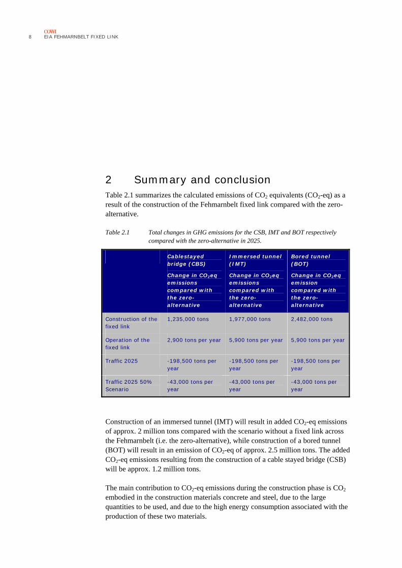
2 Summary and conclusion Table 2.1 summarizes the calculated emissions of CO2 equivalents (CO2-eq) as a result of the construction of the Fehmarnbelt fixed link compared with the zero-alternative.
Table 2.1 Total changes in GHG emissions for the CSB, IMT and BOT respectively compared with the zero-alternative in 2025.
Cablestayed bridge (CBS)
Change in CO2eq emissions compared with the zero-alternative
Immersed tunnel (IMT)
Change in CO2eq emissions compared with the zero-alternative
Bored tunnel (BOT)
Change in CO2eq emission compared with the zero-alternative
Construction of the fixed link
1,235,000 tons 1,977,000 tons 2,482,000 tons
Operation of the fixed link
2,900 tons per year 5,900 tons per year 5,900 tons per year
Traffic 2025 -198,500 tons per year
-198,500 tons per year
-198,500 tons per year
Traffic 2025 50% Scenario
-43,000 tons per year
-43,000 tons per year
-43,000 tons per year
Construction of an immersed tunnel (IMT) will result in added CO2-eq emissions of approx. 2 million tons compared with the scenario without a fixed link across the Fehmarnbelt (i.e. the zero-alternative), while construction of a bored tunnel (BOT) will result in an emission of CO2-eq of approx. 2.5 million tons. The added CO2-eq emissions resulting from the construction of a cable stayed bridge (CSB) will be approx. 1.2 million tons.
The main contribution to CO2-eq emissions during the construction phase is CO2 embodied in the construction materials concrete and steel, due to the large quantities to be used, and due to the high energy consumption associated with the production of these two materials.
EIA FEHMARNBELT FIXED LINK
9
The calculated GHG emissions from the construction of the CSB account for around 2.2%, from the construction of the IMT for around 3% and the BOT for around 4% of the total Danish CO2 eq emissions in 2009 (NERI, 2011).
If GHG emissions during construction are distributed equally over a period of 5.5 years, they correspond, in the case of an IMT, to annual emissions from 32,000 average Danes, in the case of a BOT from 44,000 average Danes, and in the case of a CSB from 23,000 average Danes.
For the CSB, embodied CO2 in reinforcement and steel is the main contributor accounting for 62% of the GHG emission from construction. Concrete contributes 17%, transport of materials 9% and machinery 7%. Other contributors are less significant.
For the IMT, CO2 embodied in concrete is the main contributor with 42% of the GHG emission from the IMT construction works. CO2 embodied in reinforcement and steel contributes another 25%. Machinery contributes 14% and transport contributes 4%, while other sources together contribute 5%.
CO2 embodied in concrete is the main contributor with 39% of the total GHG emission from construction works for the BOT. Another important source is CO2 embodied in steel for reinforcement etc., which contributes another 24%. Electricity consumption (tunnel excavation) contributes 23%, while machinery accounts for 7% and transport for 4% of the GHG emission. Other contributors are relatively insignificant.
During operation of the link, the annual CO2 emissions resulting from electricity consumption, maintenance and reinvestment activities amount to approximately 6,000 tons for the IMT and the BOT, and approximately 3,000 tons for the CSB. Over the lifetime (120 years) of the link, assuming the same emission and emission factors, these figures add up to 0.7 million ton CO 2 for the tunnel solutions and 0.35 million ton CO2 for the bridge.
Comparing the fixed link with continuous ferry operations, the fixed link will provide annual savings in CO2 emissions of approx. 200,000 tons in 2025 and 220,000 tons in 2030.
The largest savings will come from the expected closing down of ferry operations between Rødby and Puttgarden and from a reduction in ferry departures at the routes Trelleborg-Rostock and Gedser Rostock. Emission reductions will also be achieved from road and rail freight transport due to the expected transfer of road freight to rail and shorter travel distances for rail freight.
Even if the ferries at Rødby-Puttgarden continue operating, the project alternative will result in reduced CO2 traffic emission. This is due to expected reduced ferry departures at the other routes, and due to the expected transfer of road freight to rail and shorter travel distances for rail freight.
10 EIA FEHMARNBELT FIXED LINK
3 Methodology The methodology for the analysis has been based on the principles of a life cycle analysis as described in ex. DS/EN ISO 14040 (ISO14040) and in Corporate Accounting and Reporting Standard from World Resource Institute (WRI 2004) and as such including the GHG-emission related to the life cycle of the fixed link i.e. production of material, transport, construction and operation of the link. It also includes some of the same elements as defining the scope, carrying out the inventory and performing the assessment.
The description of the methodology used to calculate the CO2 emissions is divided into three parts:
› Construction of the fixed link, including the main structures and construction works, temporary work sites and approach links for rail and road
› Operation of the link, including electricity consumption, maintenance and reinvestment, excluding traffic
› Traffic.
To the extent possible, the greenhouse gas inventory will cover the contribution of all greenhouse gases, and the result will be presented in CO2 equivalents.
The greenhouse gases comprise carbon dioxide (CO2), methane (CH4), nitrous dioxide (N2O), hydro fluorocarbons (HFCs), per fluorocarbons (PFCs) and sulphur hexafluoride (SF6).
For the materials, the embodied CO2 emission is in most cases stated in CO2 equivalents, and the figure will thus include emission of all greenhouse gases.
For emission of electricity, a CO2 equivalent factor is calculated using global warming potential values according to IPCC (NERI 2007):
› Carbon dioxide: 1 › Methane: 21 › Nitrous dioxide: 310.
EIA FEHMARNBELT FIXED LINK
11
For transport, only CO2 emissions are included, because emission of GHGs other than CO2 is assessed insignificant. The Danish National Environmental Research Institute (NERI) estimates that 95-99% of the CO2 equivalents from road transport derive from CO2 (NERI 2007). This is also assumed the case for other transport modes and for construction machinery.
In defining the scope of the analysis, the objective has been to include significant, direct sources of emissions as well as indirect sources deriving from the construction and the operation phases.
The direct GHG emission sources include:
› Emissions from construction equipment on site › Emissions from traffic.
The indirect sources include GHG emissions from:
› Electricity production › Production of main materials › Transport of materials.
The calculations thus include scope 1 (direct GHG emissions), 2 (indirect GHG emissions from consumption of purchased electricity) and 3 (other indirect emissions, such as the extraction and production of purchased materials, transport related activities from using vehicles etc.) according to the Corporate Accounting and Reporting Standard from World Resource Institute (WRI 2004).
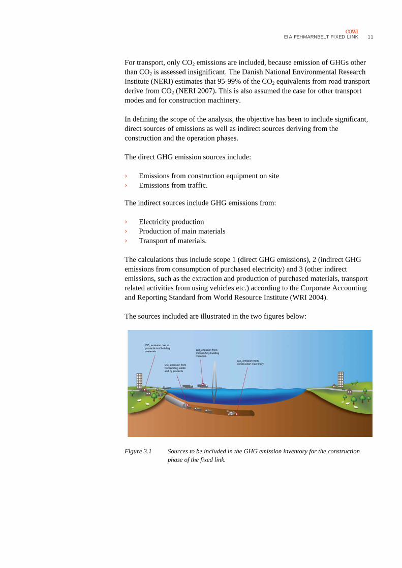
The sources included are illustrated in the two figures below:
Figure 3.1 Sources to be included in the GHG emission inventory for the construction phase of the fixed link.
12 EIA FEHMARNBELT FIXED LINK
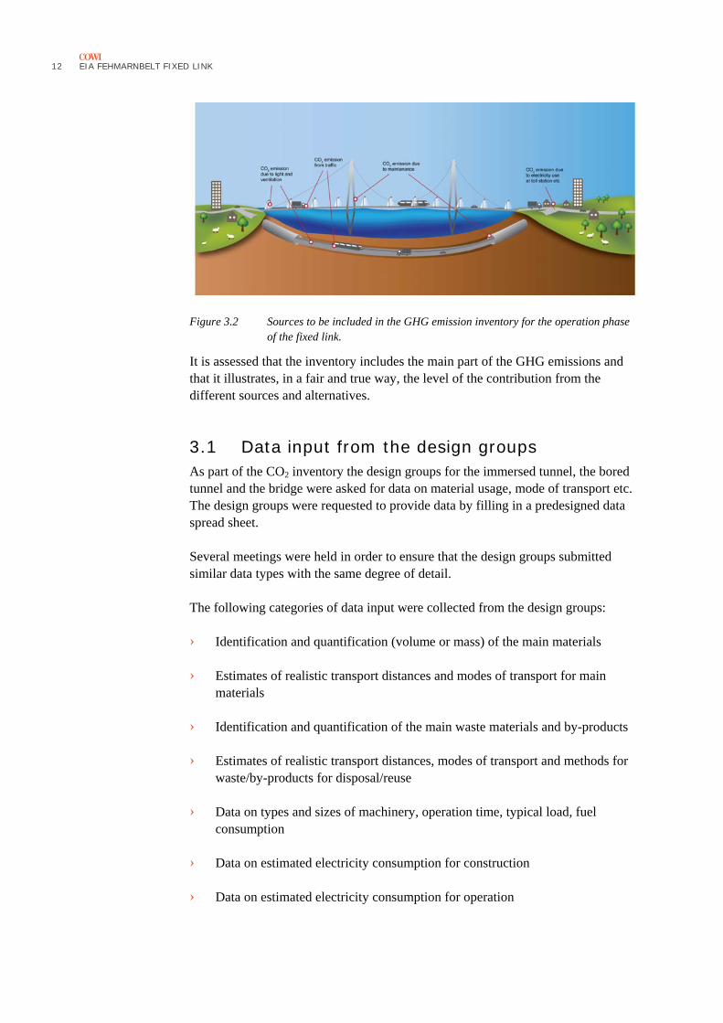
Figure 3.2 Sources to be included in the GHG emission inventory for the operation phase of the fixed link.
It is assessed that the inventory includes the main part of the GHG emissions and that it illustrates, in a fair and true way, the level of the contribution from the different sources and alternatives.
3.1 Data input from the design groups As part of the CO2 inventory the design groups for the immersed tunnel, the bored tunnel and the bridge were asked for data on material usage, mode of transport etc. The design groups were requested to provide data by filling in a predesigned data spread sheet.
Several meetings were held in order to ensure that the design groups submitted similar data types with the same degree of detail.
The following categories of data input were collected from the design groups:
› Identification and quantification (volume or mass) of the main materials
› Estimates of realistic transport distances and modes of transport for main materials
› Identification and quantification of the main waste materials and by-products
› Estimates of realistic transport distances, modes of transport and methods for waste/by-products for disposal/reuse
› Data on types and sizes of machinery, operation time, typical load, fuel consumption
› Data on estimated electricity consumption for construction
› Data on estimated electricity consumption for operation
EIA FEHMARNBELT FIXED LINK
13
› Data on the use of machines and materials for annual maintenance and planned reinvestments.
The IMT project was selected as the preferred alternative at the beginning of 2011, and the IMT design group worked continuously on the project throughout 2011, whereas the development of the bridge alternative has not progressed with the same pace. Consequently, data are more detailed and accurate for the IMT alternative than for the CSB alternative.
The BOT is not - the preferred alternative, and data are assumed to be at the same level of accuracy and detail as for the CSB.
It is assessed that the emission calculations for the three alternatives are comparable even though information about the IMT has a higher degree of detail and accuracy than the information about the CSB and BOT.
3.2 Construction of the fixed link The construction of the link comprises the main physical structures (bridge or tunnel), the construction work activities, including temporary working sites in Lolland and Fehmarn, and the approach roads and rail.
Emissions of CO2 equivalents embodied in materials, from transport of materials and from construction equipment are included in the calculations. The calculations are based on information about the quantities and the origin of the materials as estimated by the design groups.
3.2.1 Material consumption The design groups estimated the material quantities for the three alternatives.
The CO2 equivalent emission factors for the specific materials were retrieved either from literature, from databases or directly from producers. To strengthen the analysis, and wherever possible, emission factors for the specific materials were retrieved from more than one source. For further details, reference is made to a separate note about the selection of emission factors for materials (COWI 2011a).
In cases where different sources provided different emission factors for the same material, average values were adopted based on the most trustworthy sources.
The materials required for construction of the road and the railway are assumed to be identical for the IMT and BOT project alternatives.
The emission factors used for the primary materials are listed in Table 3.1.
14 EIA FEHMARNBELT FIXED LINK
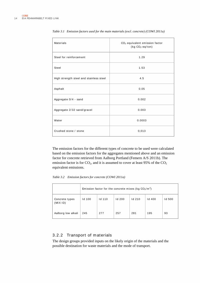
Table 3.1 Emission factors used for the main materials (excl. concrete) (COWI 2011a)
Materials CO2 equivalent emission factor (kg CO2-eq/ton)
Steel for reinforcement 1.29
Steel 1.53
High strength steel and stainless steel 4.5
Asphalt 0.05
Aggregate 0/4 - sand 0.002
Aggregate 2/32 sand/gravel 0.003
Water 0.0003
Crushed stone / stone 0,013
The emission factors for the different types of concrete to be used were calculated based on the emission factors for the aggregates mentioned above and an emission factor for concrete retrieved from Aalborg Portland (Femern A/S 2011b). The emission factor is for CO2, and it is assumed to cover at least 95% of the CO2 equivalent emissions.
Table 3.2 Emission factors for concrete (COWI 2011a)
Emission factor for the concrete mixes (kg CO2/m3)
Concrete types (MIX ID)
Id 100 Id 110 Id 200 Id 210 Id 400 Id 500
Aalborg low alkali 245 277 257 281 195 93
3.2.2 Transport of materials The design groups provided inputs on the likely origin of the materials and the possible destination for waste materials and the mode of transport.
EIA FEHMARNBELT FIXED LINK
15
In defining the transport distance and the mode of transport, the same origin and mode of transport methods were used for the same kind of materials for the two alternatives.
For the individual mode of transport, the emission factors were identified based on figures from TEMA2010 (TEMA 2010). Only CO2 emissions from the transport were included, as other GHGs would only contribute marginally to the overall CO2 equivalent emissions.
In addition, the CO2 emissions from fuel combustion were included. No upstream emissions were included.
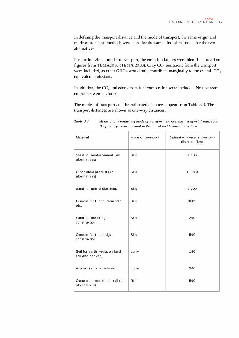
The modes of transport and the estimated distances appear from Table 3.3. The transport distances are shown as one-way distances.
Table 3.3 Assumptions regarding mode of transport and average transport distance for the primary materials used in the tunnel and bridge alternatives.
Material Mode of transport Estimated average transport distance (km)
Steel for reinforcement (all alternatives)
Ship 1,000
Other steel products (all alternatives)
Ship 15,000
Sand for tunnel elements Ship 1,000
Cement for tunnel elements etc.
Ship 900*
Sand for the bridge construction
Ship 200
Cement for the bridge construction
Ship 500
Soil for earth works on land (all alternatives)
Lorry 150
Asphalt (all alternatives) Lorry 200
Concrete elements for rail (all alternatives)
Rail 500
16 EIA FEHMARNBELT FIXED LINK
3.2.3 Use of construction machines The design groups provided estimates of the use of construction machinery – onshore and offshore – during the construction phase.
The final decision on the use of construction machinery types, sizes, numbers etc. will eventually be made by the contractors. Accordingly, best guesses were made by the design groups based on experience from similar types of projects.
The information delivered by the two design groups concerning the construction machines differed, and subsequently, the basis for the CO2 calculations has also been different.
The two tunnel design groups provided information on the main construction machinery and estimated the fuel and electricity consumption. Information on the land-based equipment for road works was not included, because its contribution to GHG emissions was found to be marginal compared with offshore machinery and equipment.
The bridge design group provided information on the main construction machinery by type and size and estimated the operation time for each group of machinery.
Where fuel consumption was not estimated by the design groups, estimates were made based on the EMEP/EEA emission inventory guidebook 2009 for Non-road mobile sources and machinery (EMEP/EEA 2010).
CO2 emissions from diesel oil were based on standard factors from the National Danish Energy Agency, Energistyrelsen (ENS 2011a).
Only CO2 emissions from the construction machinery were included, because the contribution from other GHGs is marginal. In addition, only CO2 emissions from the fuel combustion were included.
3.2.4 Electricity consumption Estimates of the electricity consumption during the construction phase for ventilation, light, pumps, compressors etc. were provided by the design groups.
The GHG emission factor for electricity was based on information on the average Danish electricity production in the period 2015-2020 projected by the National Danish Energy Agency, Energistyrelsen (ENS 2011b). It has been assumed that the GHG emission factor for electricity is the same in Denmark and Germany.
The emission factor for CO2-eq per kWh of electricity is estimated to 325 g/kWh.
3.2.5 The zero-alternative The zero-alternative is the scenario without a fixed link, but with continued ferry operations as is the case today. The zero-alternative does not encompass any new construction activities.
EIA FEHMARNBELT FIXED LINK
17
GHG emissions from ferry construction were disregarded.
3.3 Operation of the link (excluding traffic) Annual GHG emissions from the operation activities of the link (excluding traffic) originate from use of electricity for lighting, ventilation etc. and emissions from the use of materials and construction equipment for maintenance and for reinvestment.
3.3.1 Electricity consumption The annual electricity consumption for lighting, ventilation etc. during the operation of the fixed link was estimated by the design groups.
The emission factor for electricity was based on the average Danish electricity production for the year 2025 projected by the National Danish Energy Agency, Energistyrelsen (ENS 2011b).
The emission factor for CO2-eq per kWh of electricity is estimated to 266 g/kWh.
3.3.2 Maintenance and reinvestment Maintenance and reinvestment are necessary to keep the fixed link in operation for the expected lifetime of 120 years.
The design teams provided information on the use of material, equipment, electricity etc. for all planned maintenance works and reinvestments.
Maintenance was defined as the routine (daily, weekly, monthly, annual) activities to keep the rail and the road on the link in operation. Reinvestments are the more infrequent activities, which demand a relatively large reinvestment, such as new asphalt or new rail tracks etc.
The information provided by the design groups was mainly related to the use of material for renewal of example asphalt road surface, rail tracks etc. In the current stage of planning, the design groups were unable to estimate the use of equipment and transport for maintenance and reinvestment activities during operation. The contribution to GHG emissions from these sources is considered marginal and is therefore disregarded in this inventory.
The GHG emissions from maintenance and reinvestment activities were calculated as annual averages even though it is known that the activities will not be distributed evenly.
The emission factors used for materials will be the same as those mentioned in 3.2.1.
18 EIA FEHMARNBELT FIXED LINK
3.3.3 The zero-alternative The zero-alternative is the scenario without a fixed link, but with continued ferry operations as is the case today.
Input on onshore activities of ferry operations was not included in the analysis as the emission was assessed to be marginal, and no information was available (Scandlines 2009).
3.4 Traffic during operation The construction of a fixed link across the Fehmarnbelt will have significant implications for the traffic and travel pattern between Germany and Scandinavia. The fixed link will reduce travel time, thus making transport more attractive in the corridor. Therefore, a fixed link will, most likely, promote traffic and transfer transport from other routes and between modes of transport. The effects on traffic of a tunnel vs. a bridge are assumed identical.
The specific changes in traffic and transport modes in a predefined influence area were analysed by the Fehmarnbelt Traffic Consortium in 2003. The analysis was made for a fixed link alternative and a reference alternative, i.e. the zero-alternative (FTC 2003a, FTC 2003b).
Based on the traffic analysis from the FTC, an emission study was carried out in 2005 for the operation years 2015 and 2040 (COWI 2005). At that time, the planned year of inauguration of the fixed link was 2015. Emissions were calculated based on an analysis of changes in the traffic within an influence area covering Scandinavia and most of Northern Europe.
The methodology applied for this study will follow the methodology used in the 2005 study (COWI 2005).
Flight transport was included in the traffic model on the same terms as other transport modes. However, it was assessed that the effect from the change in air transport was marginal, and consequently emissions from air transport were not included in the analysis.
For further description of the model, see the reports from the Femarnbelt Traffic Consortium (FTC 2003a and FTC 2003b) and a previous report from the Danish Ministry of Transport and Energy (COWI 2005).
The GHG emission inventory emissions were calculated for the years 2025 and 2030 as determined by Femern A/S. Year 2025 and year 2030 represent years where the traffic is assumed to be phased-in and the related infrastructure projects finished.
The traffic volumes were projected using the 2015 traffic volumes (COWI 2005) as the basis assuming an annual increase in traffic of 1.7% for all traffic modes as assumed in the earlier studies (COWI 2005).
EIA FEHMARNBELT FIXED LINK
19
The emission factors for road traffic are based on assumptions for a Danish vehicle fleet composition in years 2025 and 2030, which draws on statistics and forecasts about age, size and fuel distribution.
Emission factors derive from TEMA 2010 which is the official emission calculation model by the Danish Ministry of Transport (TEMA 2010).
The traffic model is uninformative about the road types of the traffic in question. However, as the main part of the traffic involved is long-distance traffic, it has been assumed that the traffic travels on either motorways or highways.
The typical train type was defined by Femern A/S.
The basic source for the calculation of emission factors is TEMA2010. As the values are related to today’s efficiency and the technology, they have been projected to year 2025 using a reduction factor, which considers improvements in train efficiency and electricity production.
All trains are assumed fully electric.
Concerning the zero-alternative, the increase in traffic volumes across the Fehmarnbelt will determine the necessary future ferry capacity.
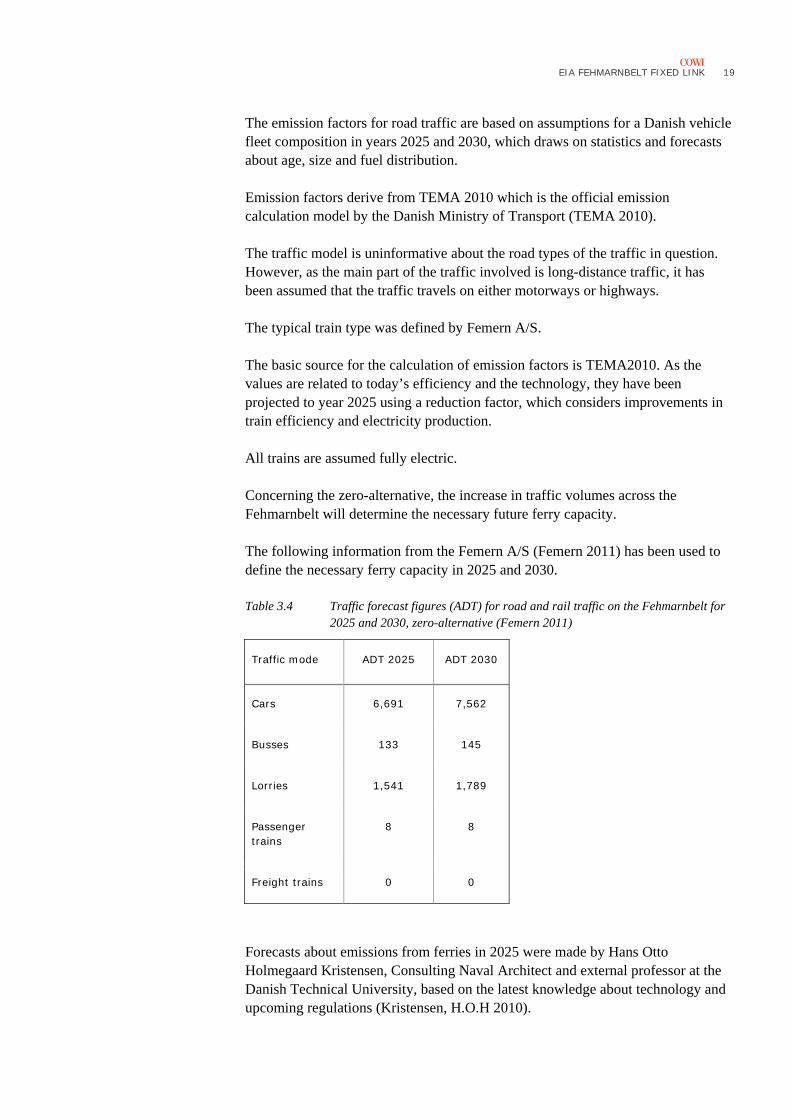
The following information from the Femern A/S (Femern 2011) has been used to define the necessary ferry capacity in 2025 and 2030.
Table 3.4 Traffic forecast figures (ADT) for road and rail traffic on the Fehmarnbelt for 2025 and 2030, zero-alternative (Femern 2011)
Traffic mode ADT 2025 ADT 2030
Cars 6,691 7,562
Busses 133 145
Lorries 1,541 1,789
Passenger trains
8 8
Freight trains 0 0
Forecasts about emissions from ferries in 2025 were made by Hans Otto Holmegaard Kristensen, Consulting Naval Architect and external professor at the Danish Technical University, based on the latest knowledge about technology and upcoming regulations (Kristensen, H.O.H 2010).
20 EIA FEHMARNBELT FIXED LINK
The predictions cover the ferry routes Rødby-Puttgarden, Trelleborg-Rostock and Gedser-Rostock.
For the year 2030, COWI has estimated the emissions based on the emission factors provided by Hans Otto Holmegaard Kristensen.
For Rødby-Puttgarden, the ferry capacity was adjusted to the expected traffic volumes using the figures stated in Table 3.4.
3.4.1 Comparison of the project alternative with the zero-alternative and a 50% scenario
The analysis quantifies the CO2 emissions from transport on a fixed link across the Fehmarnbelt compared to the zero-alternative and a so called 50% scenario. The zero-alternative, the project alternative and the 50% scenario are defined in the following.
The zero-alternative The zero-alternative is defined as an infrastructure scenario, as it would be in 2025/2030 without a fixed link across the Fehmarnbelt. The traffic in the zero-alternative is assumed to be identical to the traffic scenario named Reference Case B in FTC (2003b), only extrapolated to year 2025/2030.
It is assumed that the ferries at Rødby-Puttgarden are rebuilt to a higher capacity, and that the ferries serving the Gedser-Rostock and the Trelleborg-Rostock (fast ferry) routes have the same number of departure as today i.e. one departure a day less compared to the project alternative.
It is assumed that the Danish railway lines Vamdrup-Vojens and Tinglev-Padborg are upgraded to double tracks. Further, it is assumed that the German railway line Neumünster-Bad Oldesloe is electrified and upgraded to double tracks with a maximum speed of 120 km/h.
Moreover, a number of improvements especially of railway infrastructure are assumed – e.g. upgrading of the railway line Copenhagen-Ringsted – but these are the same in the zero-alternative and the project alternatives.
The fixed link (the project alternative) The project alternative is defined as a fixed link across the Fehmarnbelt with four road lanes and two railway tracks. At the time, when the FTC analyses were made, the fixed link was expected to be inaugurated in 2015. The project alternative is identical to the traffic scenario named Base Case B in the FTC (2003a).
It is assumed that the ferry route Rødby-Puttgarden will close down when the fixed link opens. With regards to the other routes in the analysis, they are assumed to have one departure a day less from each port.
Concerning rail traffic, it is assumed that the Danish railway line Ringsted-Rødby is electrified, and that the railway line Orehoved-Rødby is upgraded to double
EIA FEHMARNBELT FIXED LINK
21
tracks. In Germany, it is assumed that the railway line Puttgarden-Bad Schwartau is upgraded to double tracks, that the railway line Bad Oldesloe-Ahrensburg is upgraded to three tracks and that the railway line Ahrensburg-Hamburg-Wandsbek is upgraded to four tracks. Finally, the railway line Lübeck-Puttgarden is assumed electrified.
The 50% scenario The 50% scenario is the scenario, where a fixed link is established and the ferries across Fehmarnbelt continue their service at Rødby-Puttgarden as today. The traffic across the belt is assumed to be as for the project scenario, except 50% of the passenger cars will use the ferries. The ferries are assumed to be as they are today.
22 EIA FEHMARNBELT FIXED LINK
4 GHG emissions from construction of the fixed link
4.1 The immersed tunnel (IMT)
4.1.1 Data input
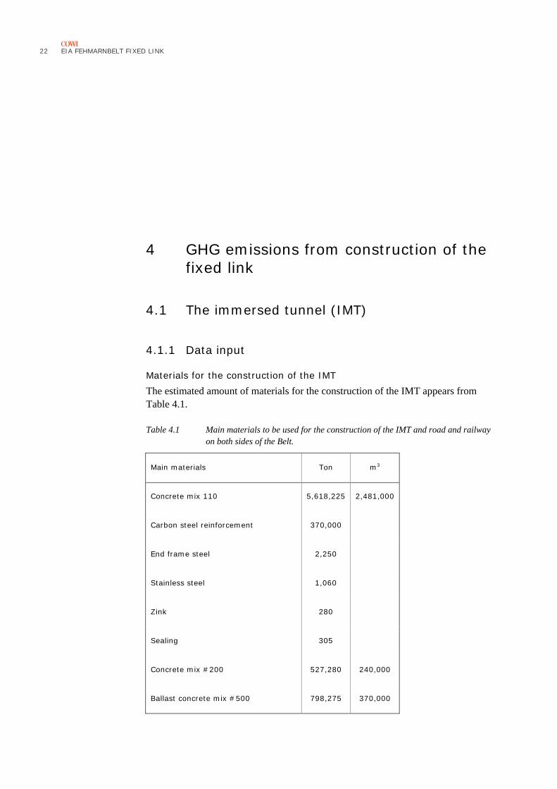
Materials for the construction of the IMT The estimated amount of materials for the construction of the IMT appears from Table 4.1.
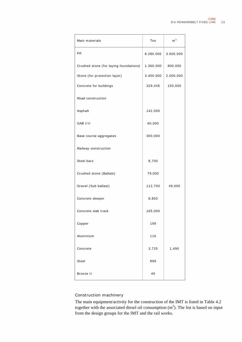
Table 4.1 Main materials to be used for the construction of the IMT and road and railway on both sides of the Belt.
Main materials Ton m3
Concrete mix 110 5,618,225 2,481,000
Carbon steel reinforcement 370,000
End frame steel 2,250
Stainless steel 1,060
Zink 280
Sealing 305
Concrete mix #200 527,280 240,000
Ballast concrete mix #500 798,275 370,000
EIA FEHMARNBELT FIXED LINK
23
Main materials Ton m3
Fill 8.280.000 3.600.000
Crushed stone (for laying foundations) 1.360.000 800.000
Stone (for protection layer) 3.400.000 2.000.000
Concrete for buildings 329,445 150,000
Road construction
Asphalt 142,000
GAB I/II 60,000
Base course aggregates 300,000
Railway construction
Steel bars 8,700
Crushed stone (Ballast) 79,000
Gravel (Sub ballast) 112,700 49,000
Concrete sleeper 8,850
Concrete slab track 165,000
Copper 199
Aluminium 116
Concrete 3,725 1,490
Steel 899
Bronze II 40
Construction machinery The main equipment/activity for the construction of the IMT is listed in Table 4.2 together with the associated diesel oil consumption (m3). The list is based on input from the design groups for the IMT and the rail works.
24 EIA FEHMARNBELT FIXED LINK
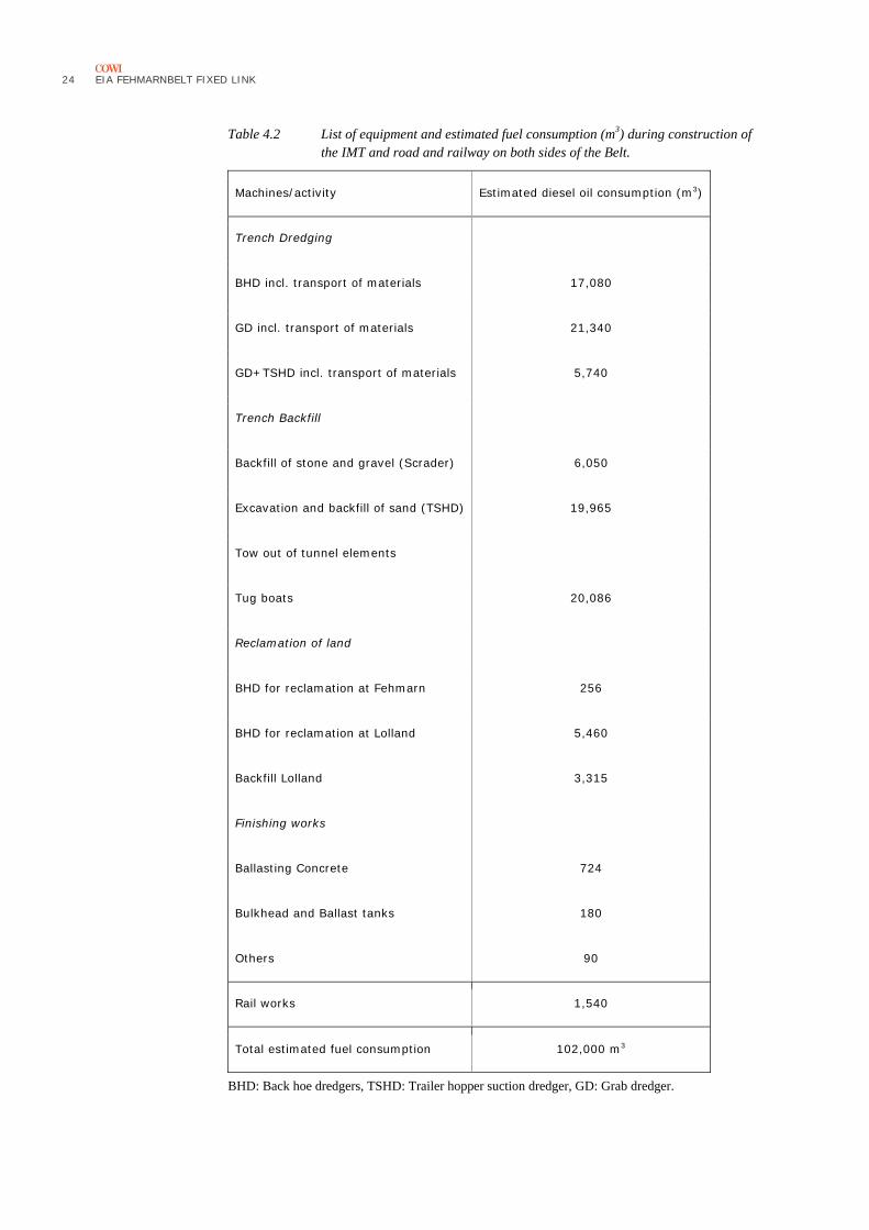
Table 4.2 List of equipment and estimated fuel consumption (m3) during construction of the IMT and road and railway on both sides of the Belt.
Machines/activity Estimated diesel oil consumption (m3)
Trench Dredging
BHD incl. transport of materials 17,080
GD incl. transport of materials 21,340
GD+TSHD incl. transport of materials 5,740
Trench Backfill
Backfill of stone and gravel (Scrader) 6,050
Excavation and backfill of sand (TSHD) 19,965
Tow out of tunnel elements
Tug boats 20,086
Reclamation of land
BHD for reclamation at Fehmarn 256
BHD for reclamation at Lolland 5,460
Backfill Lolland 3,315
Finishing works
Ballasting Concrete 724
Bulkhead and Ballast tanks 180
Others 90
Rail works 1,540
Total estimated fuel consumption 102,000 m3
BHD: Back hoe dredgers, TSHD: Trailer hopper suction dredger, GD: Grab dredger.
EIA FEHMARNBELT FIXED LINK
25
Excavation and backfill of sand with TSHD include excavation of sand at Kriegers Flak and transport and backfill at the site at Fehmarnbelt.
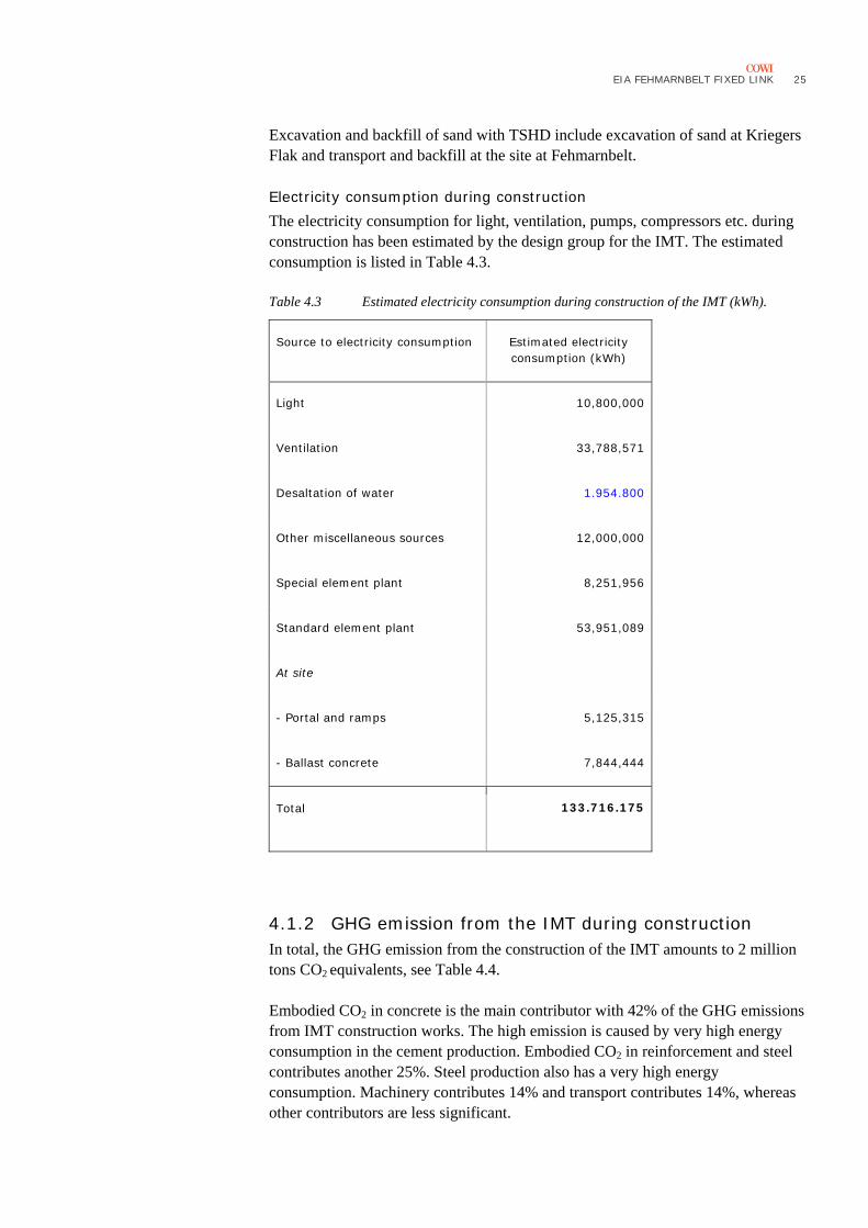
Electricity consumption during construction The electricity consumption for light, ventilation, pumps, compressors etc. during construction has been estimated by the design group for the IMT. The estimated consumption is listed in Table 4.3.
Table 4.3 Estimated electricity consumption during construction of the IMT (kWh).
Source to electricity consumption Estimated electricity consumption (kWh)
Light 10,800,000
Ventilation 33,788,571
Desaltation of water 1.954.800
Other miscellaneous sources 12,000,000
Special element plant 8,251,956
Standard element plant 53,951,089
At site
- Portal and ramps 5,125,315
- Ballast concrete 7,844,444
Total 133.716.175
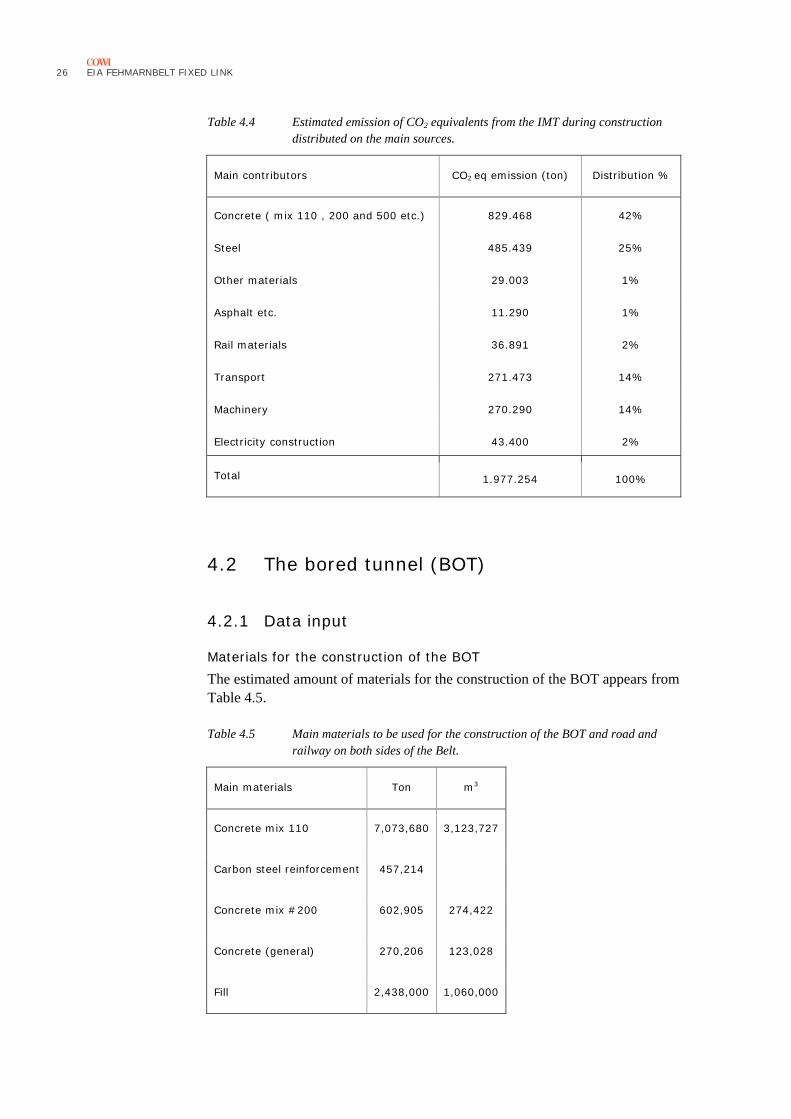
4.1.2 GHG emission from the IMT during construction In total, the GHG emission from the construction of the IMT amounts to 2 million tons CO2 equivalents, see Table 4.4.
Embodied CO2 in concrete is the main contributor with 42% of the GHG emissions from IMT construction works. The high emission is caused by very high energy consumption in the cement production. Embodied CO2 in reinforcement and steel contributes another 25%. Steel production also has a very high energy consumption. Machinery contributes 14% and transport contributes 14%, whereas other contributors are less significant.
26 EIA FEHMARNBELT FIXED LINK
Table 4.4 Estimated emission of CO2 equivalents from the IMT during construction distributed on the main sources.
Main contributors CO2 eq emission (ton) Distribution %
Concrete ( mix 110 , 200 and 500 etc.) 829.468 42%
Steel 485.439 25%
Other materials 29.003 1%
Asphalt etc. 11.290 1%
Rail materials 36.891 2%
Transport 271.473 14%
Machinery 270.290 14%
Electricity construction 43.400 2%
Total 1.977.254 100%
4.2 The bored tunnel (BOT)
4.2.1 Data input
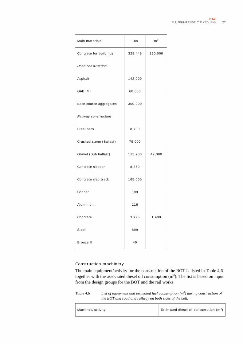
Materials for the construction of the BOT The estimated amount of materials for the construction of the BOT appears from Table 4.5.
Table 4.5 Main materials to be used for the construction of the BOT and road and railway on both sides of the Belt.
Main materials Ton m3
Concrete mix 110 7,073,680 3,123,727
Carbon steel reinforcement 457,214
Concrete mix #200 602,905 274,422
Concrete (general) 270,206 123,028
Fill 2,438,000 1,060,000
EIA FEHMARNBELT FIXED LINK
27
Main materials Ton m3
Concrete for buildings 329,445 150,000
Road construction
Asphalt 142,000
GAB I/II 60,000
Base course aggregates 300,000
Railway construction
Steel bars 8,700
Crushed stone (Ballast) 79,000
Gravel (Sub ballast) 112,700 49,000
Concrete sleeper 8,850
Concrete slab track 165,000
Copper 199
Aluminium 116
Concrete 3,725 1,490
Steel 899
Bronze II 40
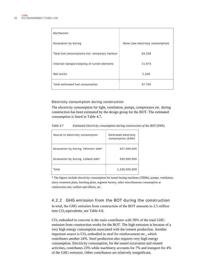
Construction machinery The main equipment/activity for the construction of the BOT is listed in Table 4.6 together with the associated diesel oil consumption (m3). The list is based on input from the design groups for the BOT and the rail works.
Table 4.6 List of equipment and estimated fuel consumption (m3) during construction of the BOT and road and railway on both sides of the belt.
Machines/activity Estimated diesel oil consumption (m3)
28 EIA FEHMARNBELT FIXED LINK
Earthworks
Excavation by boring None (see electricity consumption)
Total fuel consumptions incl. temporary harbour 54,228
Internal transport/placing of tunnel elements 11,974
Rail works 1,540
Total estimated fuel consumption 67,750
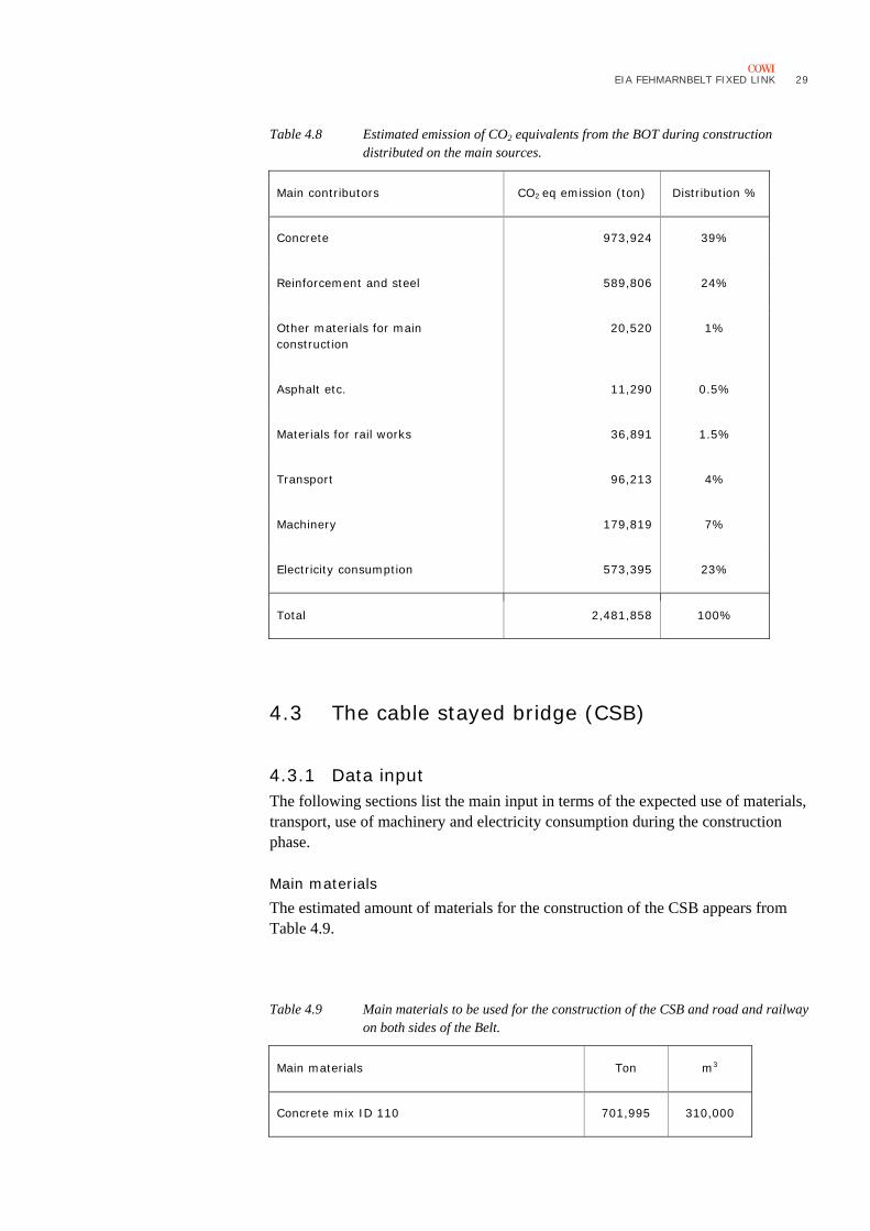
Electricity consumption during construction The electricity consumption for light, ventilation, pumps, compressors etc. during construction has been estimated by the design group for the BOT. The estimated consumption is listed in Table 4.7.
Table 4.7 Estimated electricity consumption during construction of the BOT (kWh).
Source to electricity consumption Estimated electricity consumption (kWh)
Excavation by boring, Fehmarn side* 637,000,000
Excavation by boring, Lolland side* 593,000,000
Total 1,230,000,000
* The figures include electricity consumption for tunnel boring machines (TBMs), pumps, ventilation,
slurry treatment plant, batching plant, segment factory, other miscellaneous consumption at
construction site, welfare and offices, etc.
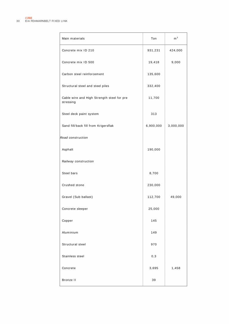
4.2.2 GHG emission from the BOT during the construction In total, the GHG emission from construction of the BOT amounts to 2.5 million tons CO2 equivalents, see Table 4.8.
CO2 embodied in concrete is the main contributor with 39% of the total GHG emission from construction works for the BOT. The high emission is because of a very high energy consumption associated with the cement production. Another important source is CO2 embodied in steel for reinforcement etc., which contributes another 24%. Steel production also requires very high energy consumption. Electricity consumption, for the tunnel excavation and related activities, contributes 23% while machinery accounts for 7% and transport for 4% of the GHG emission. Other contributors are relatively insignificant.
EIA FEHMARNBELT FIXED LINK
29
Table 4.8 Estimated emission of CO2 equivalents from the BOT during construction distributed on the main sources.
Main contributors CO2 eq emission (ton) Distribution %
Concrete 973,924 39%
Reinforcement and steel 589,806 24%
Other materials for main construction
20,520 1%
Asphalt etc. 11,290 0.5%
Materials for rail works 36,891 1.5%
Transport 96,213 4%
Machinery 179,819 7%
Electricity consumption 573,395 23%
Total 2,481,858 100%
4.3 The cable stayed bridge (CSB)
4.3.1 Data input The following sections list the main input in terms of the expected use of materials, transport, use of machinery and electricity consumption during the construction phase.
Main materials The estimated amount of materials for the construction of the CSB appears from Table 4.9.
Table 4.9 Main materials to be used for the construction of the CSB and road and railway on both sides of the Belt.
Main materials Ton m3
Concrete mix ID 110 701,995 310,000
30 EIA FEHMARNBELT FIXED LINK
Main materials Ton m3
Concrete mix ID 210 931,231 424,000
Concrete mix ID 500 19,418 9,000
Carbon steel reinforcement 135,600
Structural steel and steel piles 332,400
Cable wire and High Strength steel for pre stressing
11,700
Steel deck paint system 313
Sand fill/back fill from Krigersflak 6,900,000 3,000,000
Road construction
Asphalt 190,000
Railway construction
Steel bars 8,700
Crushed stone 230,000
Gravel (Sub ballast) 112,700 49,000
Concrete sleeper 25,000
Copper 145
Aluminium 149
Structural steel 970
Stainless steel 0,3
Concrete 3,695 1,458
Bronze II 39
EIA FEHMARNBELT FIXED LINK
31
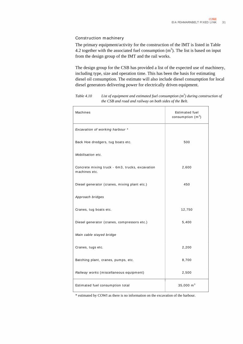
Construction machinery The primary equipment/activity for the construction of the IMT is listed in Table 4.2 together with the associated fuel consumption (m3). The list is based on input from the design group of the IMT and the rail works.
The design group for the CSB has provided a list of the expected use of machinery, including type, size and operation time. This has been the basis for estimating diesel oil consumption. The estimate will also include diesel consumption for local diesel generators delivering power for electrically driven equipment.
Table 4.10 List of equipment and estimated fuel consumption (m3) during construction of the CSB and road and railway on both sides of the Belt.
Machines Estimated fuel consumption (m3)
Excavation of working harbour *
Back Hoe dredgers, tug boats etc. 500
Mobilisation etc.
Concrete mixing truck - 6m3, trucks, excavation machines etc.
2,600
Diesel generator (cranes, mixing plant etc.) 450
Approach bridges
Cranes, tug boats etc. 12,750
Diesel generator (cranes, compressors etc.) 5,400
Main cable stayed bridge
Cranes, tugs etc. 2,200
Batching plant, cranes, pumps, etc. 8,700
Railway works (miscellaneous equipment) 2,500
Estimated fuel consumption total 35,000 m3
* estimated by COWI as there is no information on the excavation of the harbour.
32 EIA FEHMARNBELT FIXED LINK
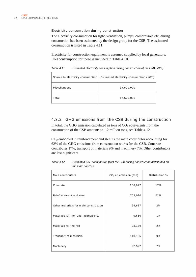
Electricity consumption during construction The electricity consumption for light, ventilation, pumps, compressors etc. during construction has been estimated by the design group for the CSB. The estimated consumption is listed in Table 4.11.
Electricity for construction equipment is assumed supplied by local generators. Fuel consumption for these is included in Table 4.10.
Table 4.11 Estimated electricity consumption during construction of the CSB (kWh).
Source to electricity consumption Estimated electricity consumption (kWh)
Miscellaneous 17,520,000
Total 17,520,000
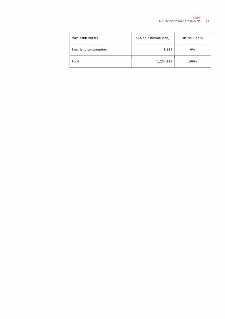
4.3.2 GHG emissions from the CSB during the construction In total, the GHG emission calculated as tons of CO2 equivalents from the construction of the CSB amounts to 1.2 million tons, see Table 4.12.
CO2 embodied in reinforcement and steel is the main contributor accounting for 62% of the GHG emissions from construction works for the CSB. Concrete contributes 17%, transport of materials 9% and machinery 7%. Other contributors are less significant.
Table 4.12 Estimated CO2 contribution from the CSB during construction distributed on the main sources.
Main contributors CO2-eq emission (ton) Distribution %
Concrete 206,027 17%
Reinforcement and steel 763,020 62%
Other materials for main construction 24,637 2%
Materials for the road, asphalt etc. 9,660 1%
Materials for the rail 23,189 2%
Transport of materials 110,155 9%
Machinery 92,522 7%
EIA FEHMARNBELT FIXED LINK
33
Main contributors CO2-eq emission (ton) Distribution %
Electricity consumption 5,686 0%
Total 1,234,896 100%
34 EIA FEHMARNBELT FIXED LINK
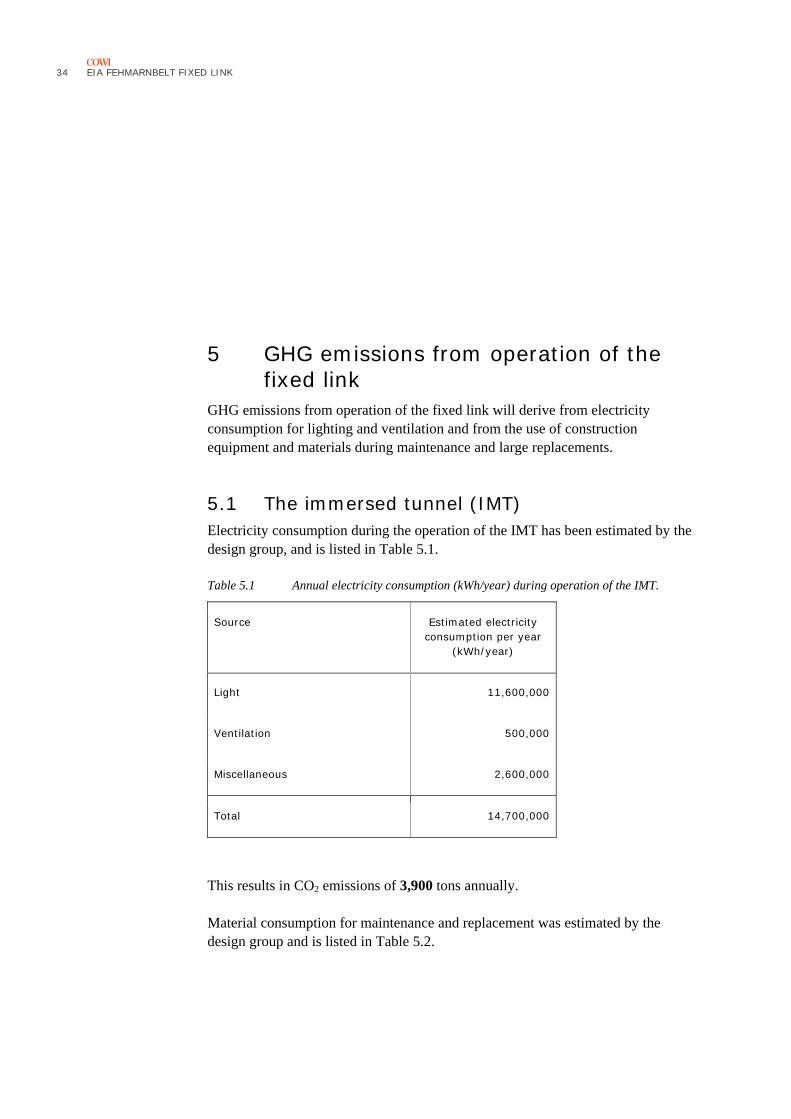
5 GHG emissions from operation of the fixed link
GHG emissions from operation of the fixed link will derive from electricity consumption for lighting and ventilation and from the use of construction equipment and materials during maintenance and large replacements.
5.1 The immersed tunnel (IMT) Electricity consumption during the operation of the IMT has been estimated by the design group, and is listed in Table 5.1.
Table 5.1 Annual electricity consumption (kWh/year) during operation of the IMT.
Source Estimated electricity consumption per year
(kWh/year)
Light 11,600,000
Ventilation 500,000
Miscellaneous 2,600,000
Total 14,700,000
This results in CO2 emissions of 3,900 tons annually.
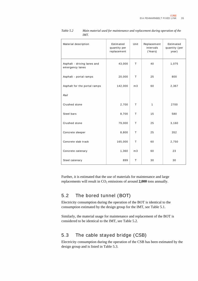
Material consumption for maintenance and replacement was estimated by the design group and is listed in Table 5.2.
EIA FEHMARNBELT FIXED LINK
35
Table 5.2 Main material used for maintenance and replacement during operation of the IMT.
Material description Estimated quantity per replacement
Unit Replacement intervals (Years)
Estimated quantity (per
year)
Asphalt - driving lanes and emergency lanes
43,000 T 40 1,075
Asphalt - portal ramps 20,000 T 25 800
Asphalt for the portal ramps 142,000 m3 60 2,367
Rail
Crushed stone 2,700 T 1 2700
Steel bars 8,700 T 15 580
Crushed stone 79,000 T 25 3,160
Concrete sleeper 8,800 T 25 352
Concrete slab track 165,000 T 60 2,750
Concrete catenary 1,360 m3 60 23
Steel catenary 899 T 30 30
Further, it is estimated that the use of materials for maintenance and large replacements will result in CO2 emissions of around 2,000 tons annually.
5.2 The bored tunnel (BOT) Electricity consumption during the operation of the BOT is identical to the consumption estimated by the design group for the IMT, see Table 5.1.
Similarly, the material usage for maintenance and replacement of the BOT is considered to be identical to the IMT, see Table 5.2.
5.3 The cable stayed bridge (CSB) Electricity consumption during the operation of the CSB has been estimated by the design group and is listed in Table 5.3.
36 EIA FEHMARNBELT FIXED LINK
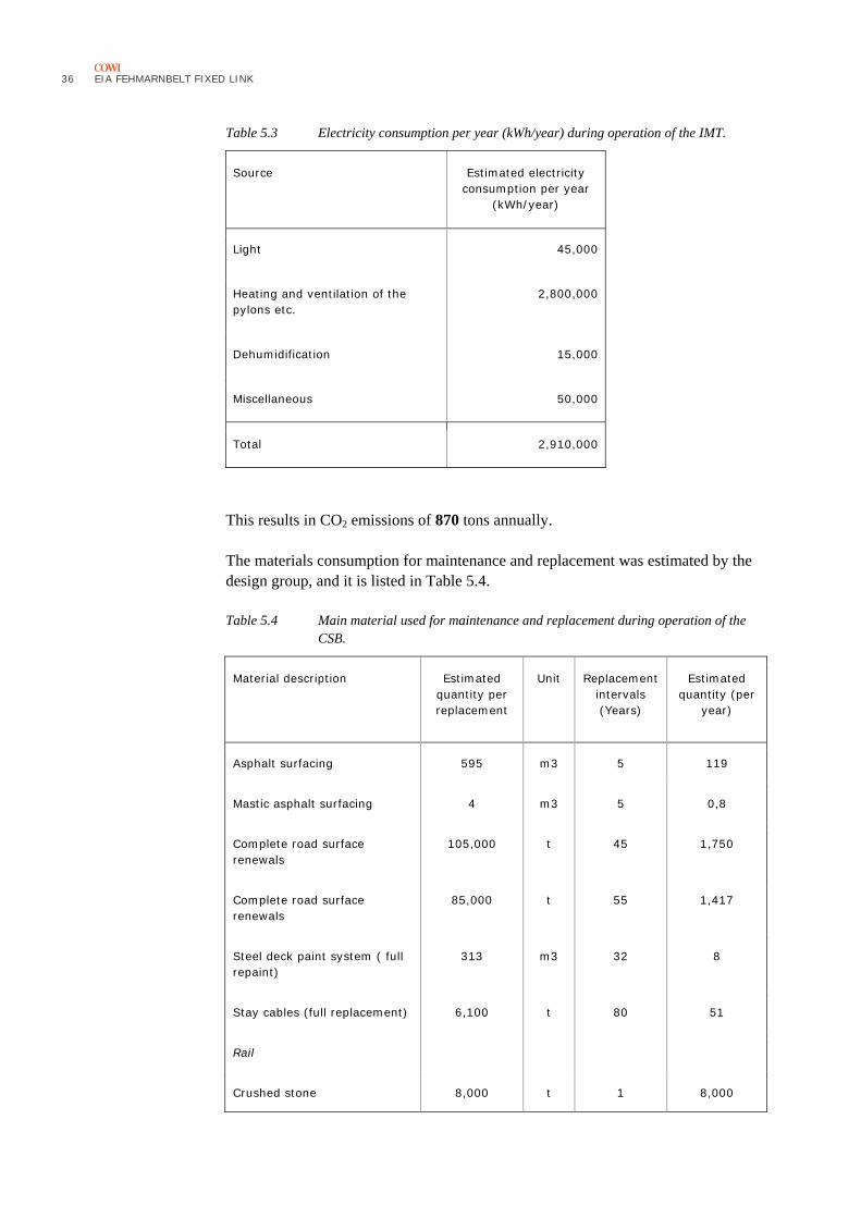
Table 5.3 Electricity consumption per year (kWh/year) during operation of the IMT.
Source Estimated electricity consumption per year
(kWh/year)
Light 45,000
Heating and ventilation of the pylons etc.
2,800,000
Dehumidification 15,000
Miscellaneous 50,000
Total 2,910,000
This results in CO2 emissions of 870 tons annually.
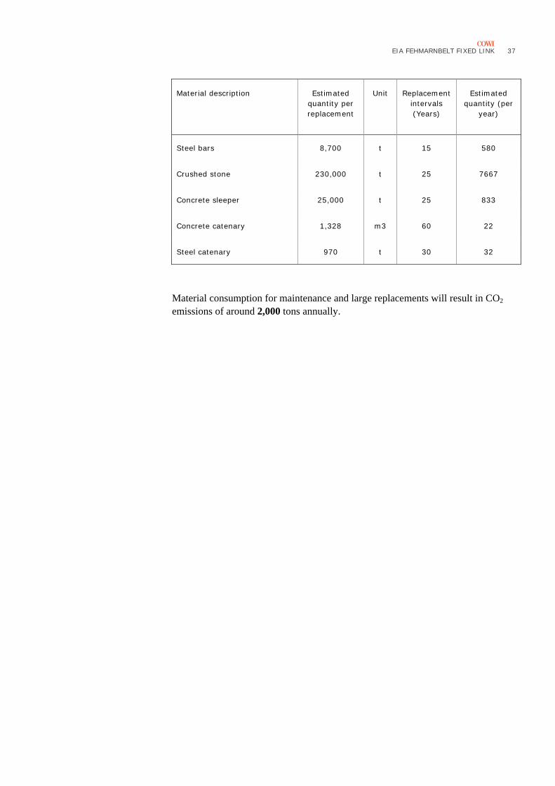
The materials consumption for maintenance and replacement was estimated by the design group, and it is listed in Table 5.4.
Table 5.4 Main material used for maintenance and replacement during operation of the CSB.
Material description Estimated quantity per replacement
Unit Replacement intervals (Years)
Estimated quantity (per
year)
Asphalt surfacing 595 m3 5 119
Mastic asphalt surfacing 4 m3 5 0,8
Complete road surface renewals
105,000 t 45 1,750
Complete road surface renewals
85,000 t 55 1,417
Steel deck paint system ( full repaint)
313 m3 32 8
Stay cables (full replacement) 6,100 t 80 51
Rail
Crushed stone 8,000 t 1 8,000
EIA FEHMARNBELT FIXED LINK
37
Material description Estimated quantity per replacement
Unit Replacement intervals (Years)
Estimated quantity (per
year)
Steel bars 8,700 t 15 580
Crushed stone 230,000 t 25 7667
Concrete sleeper 25,000 t 25 833
Concrete catenary 1,328 m3 60 22
Steel catenary 970 t 30 32
Material consumption for maintenance and large replacements will result in CO2 emissions of around 2,000 tons annually.
38 EIA FEHMARNBELT FIXED LINK
6 CO2 emission from traffic
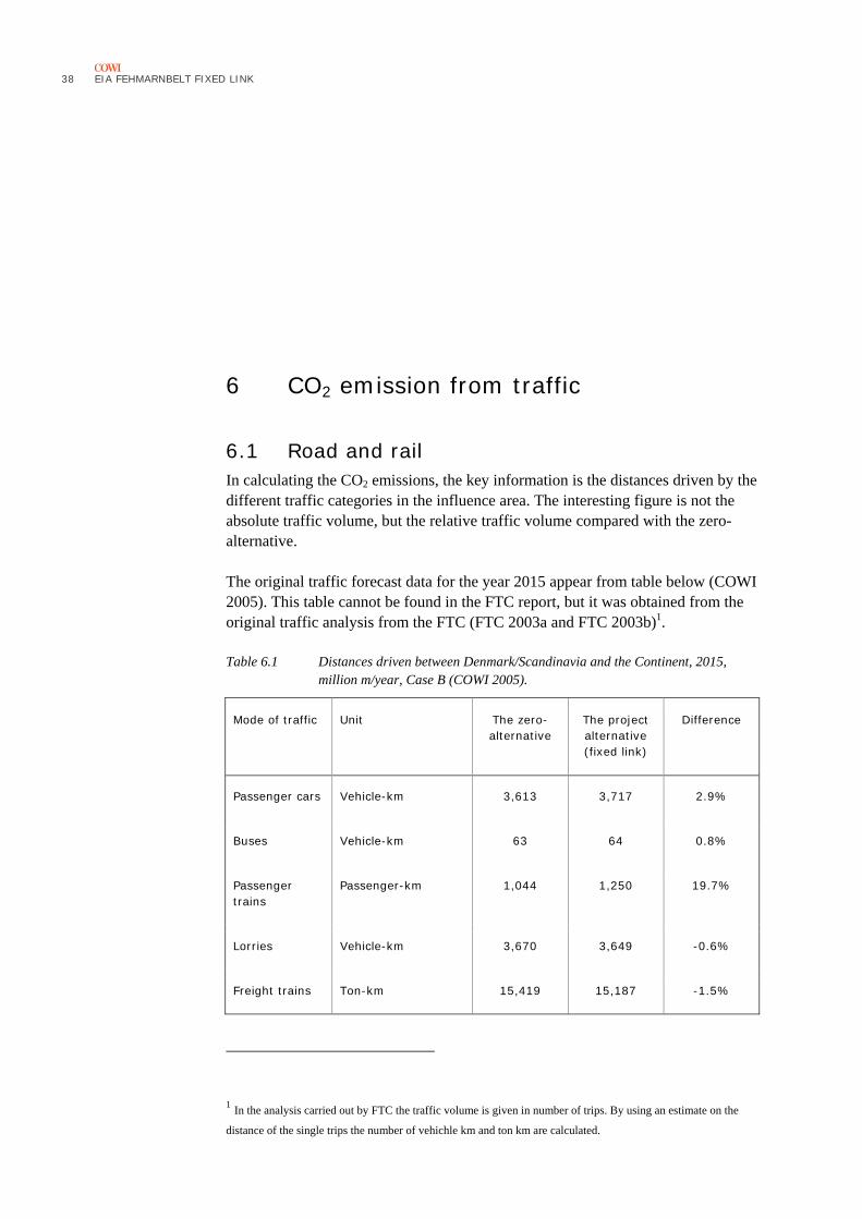
6.1 Road and rail In calculating the CO2 emissions, the key information is the distances driven by the different traffic categories in the influence area. The interesting figure is not the absolute traffic volume, but the relative traffic volume compared with the zero-alternative.
The original traffic forecast data for the year 2015 appear from table below (COWI 2005). This table cannot be found in the FTC report, but it was obtained from the original traffic analysis from the FTC (FTC 2003a and FTC 2003b)1.
Table 6.1 Distances driven between Denmark/Scandinavia and the Continent, 2015, million m/year, Case B (COWI 2005).
Mode of traffic Unit The zero-alternative
The project alternative (fixed link)
Difference
Passenger cars Vehicle-km 3,613 3,717 2.9%
Buses Vehicle-km 63 64 0.8%
Passenger trains
Passenger-km 1,044 1,250 19.7%
Lorries Vehicle-km 3,670 3,649 -0.6%
Freight trains Ton-km 15,419 15,187 -1.5%
1 In the analysis carried out by FTC the traffic volume is given in number of trips. By using an estimate on the
distance of the single trips the number of vehichle km and ton km are calculated.
EIA FEHMARNBELT FIXED LINK
39
Mode of traffic Unit The zero-alternative
The project alternative (fixed link)
Difference
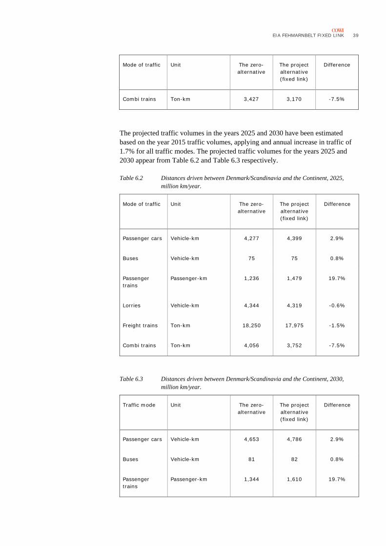
Combi trains Ton-km 3,427 3,170 -7.5%
The projected traffic volumes in the years 2025 and 2030 have been estimated based on the year 2015 traffic volumes, applying and annual increase in traffic of 1.7% for all traffic modes. The projected traffic volumes for the years 2025 and 2030 appear from Table 6.2 and Table 6.3 respectively.
Table 6.2 Distances driven between Denmark/Scandinavia and the Continent, 2025, million km/year.
Mode of traffic Unit The zero-alternative
The project alternative (fixed link)
Difference
Passenger cars Vehicle-km 4,277 4,399 2.9%
Buses Vehicle-km 75 75 0.8%
Passenger trains
Passenger-km 1,236 1,479 19.7%
Lorries Vehicle-km 4,344 4,319 -0.6%
Freight trains Ton-km 18,250 17,975 -1.5%
Combi trains Ton-km 4,056 3,752 -7.5%
Table 6.3 Distances driven between Denmark/Scandinavia and the Continent, 2030, million km/year.
Traffic mode Unit The zero-alternative
The project alternative (fixed link)
Difference
Passenger cars Vehicle-km 4,653 4,786 2.9%
Buses Vehicle-km 81 82 0.8%
Passenger trains
Passenger-km 1,344 1,610 19.7%
40 EIA FEHMARNBELT FIXED LINK
Traffic mode Unit The zero-alternative
The project alternative (fixed link)
Difference
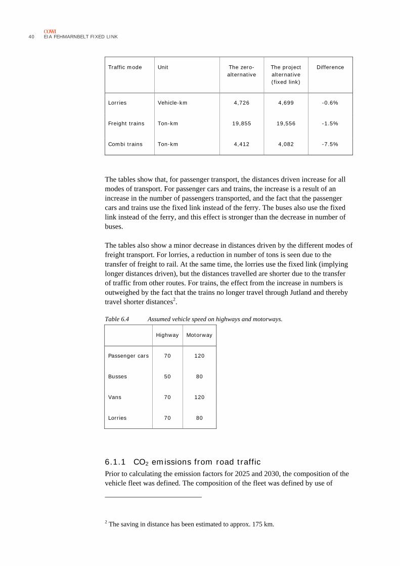
Lorries Vehicle-km 4,726 4,699 -0.6%
Freight trains Ton-km 19,855 19,556 -1.5%
Combi trains Ton-km 4,412 4,082 -7.5%
The tables show that, for passenger transport, the distances driven increase for all modes of transport. For passenger cars and trains, the increase is a result of an increase in the number of passengers transported, and the fact that the passenger cars and trains use the fixed link instead of the ferry. The buses also use the fixed link instead of the ferry, and this effect is stronger than the decrease in number of buses.
The tables also show a minor decrease in distances driven by the different modes of freight transport. For lorries, a reduction in number of tons is seen due to the transfer of freight to rail. At the same time, the lorries use the fixed link (implying longer distances driven), but the distances travelled are shorter due to the transfer of traffic from other routes. For trains, the effect from the increase in numbers is outweighed by the fact that the trains no longer travel through Jutland and thereby travel shorter distances2.
Table 6.4 Assumed vehicle speed on highways and motorways.
Highway Motorway
Passenger cars 70 120
Busses 50 80
Vans 70 120
Lorries 70 80
6.1.1 CO2 emissions from road traffic Prior to calculating the emission factors for 2025 and 2030, the composition of the vehicle fleet was defined. The composition of the fleet was defined by use of
2 The saving in distance has been estimated to approx. 175 km.
EIA FEHMARNBELT FIXED LINK
41
statistics and knowledge about vehicle size, fuel and age distribution etc. Emission factors have been calculated for the typical driving pattern on motorways and highways respectively. The default driving speeds for the two road types are applied in the calculations. Table 6.4 presents the assumptions for the speed of the road traffic.
In calculating the effect on air emissions from road transport, the emission factors for motorways and highways are weighted together. A 50/50 split is assumed in the basic calculation.
Passenger cars For passenger cars, the data from TEMA2010 are categorized by:
› Fuel
› Euro norm
› Size
› Road type.
Concerning fuel consumption and CO2 emissions, the TEMA2010 data apply to 2010 technology.
The data from TEMA2010 operate with two types of fuel: petrol and diesel. For petrol cars, the current CO2 emission factors include the addition of 5% ethanol.
In the future, this is most likely to change, as the EU goal is to increase the share of biofuels to at least 10% of petrol and diesel in 2020.
Consequently, a reduction factor has been applied to the TEMA2010 fuel consumption factor, and the CO2 emission factor was reduced by 3% for petrol vehicles and 5% for the diesel vehicles%.
Electric passenger cars were excluded from the analysis due to very uncertain developments in this technology (COWI 2010). Further, as the trips included in this analysis were assumed to be long-distance trips, electric cars were not considered a very likely choice.
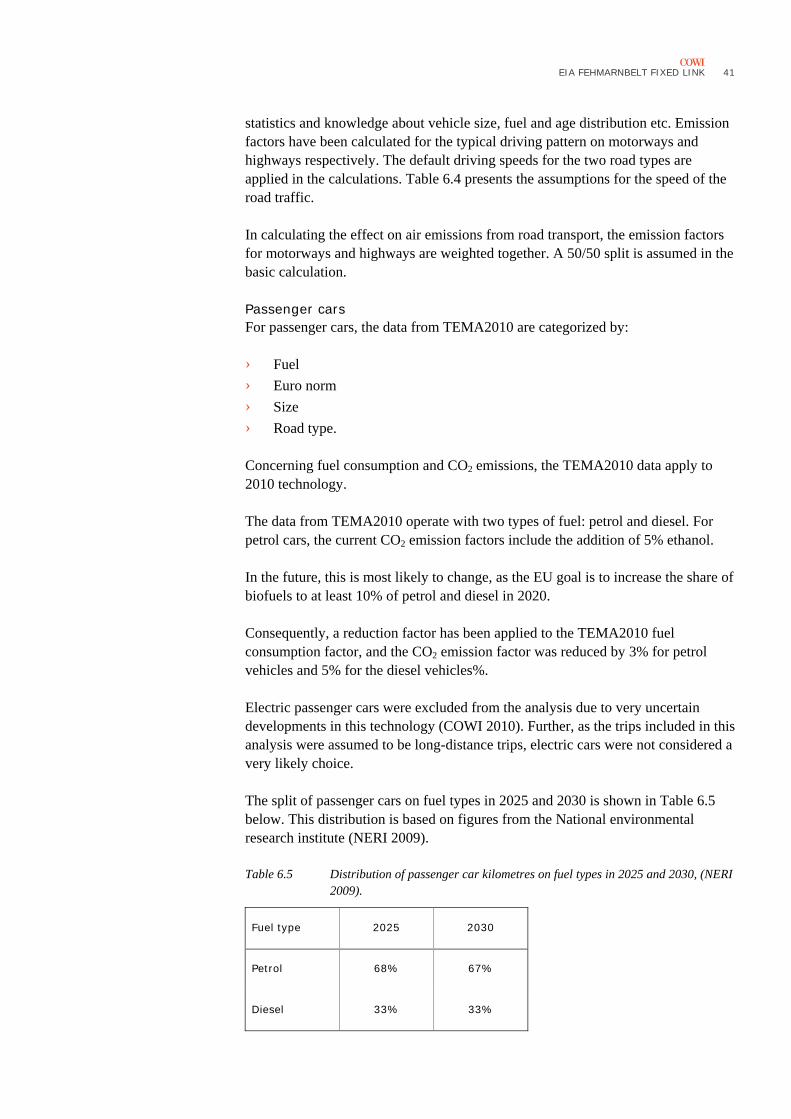
The split of passenger cars on fuel types in 2025 and 2030 is shown in Table 6.5 below. This distribution is based on figures from the National environmental research institute (NERI 2009).
Table 6.5 Distribution of passenger car kilometres on fuel types in 2025 and 2030, (NERI 2009).
Fuel type 2025 2030
Petrol 68% 67%
Diesel 33% 33%
42 EIA FEHMARNBELT FIXED LINK
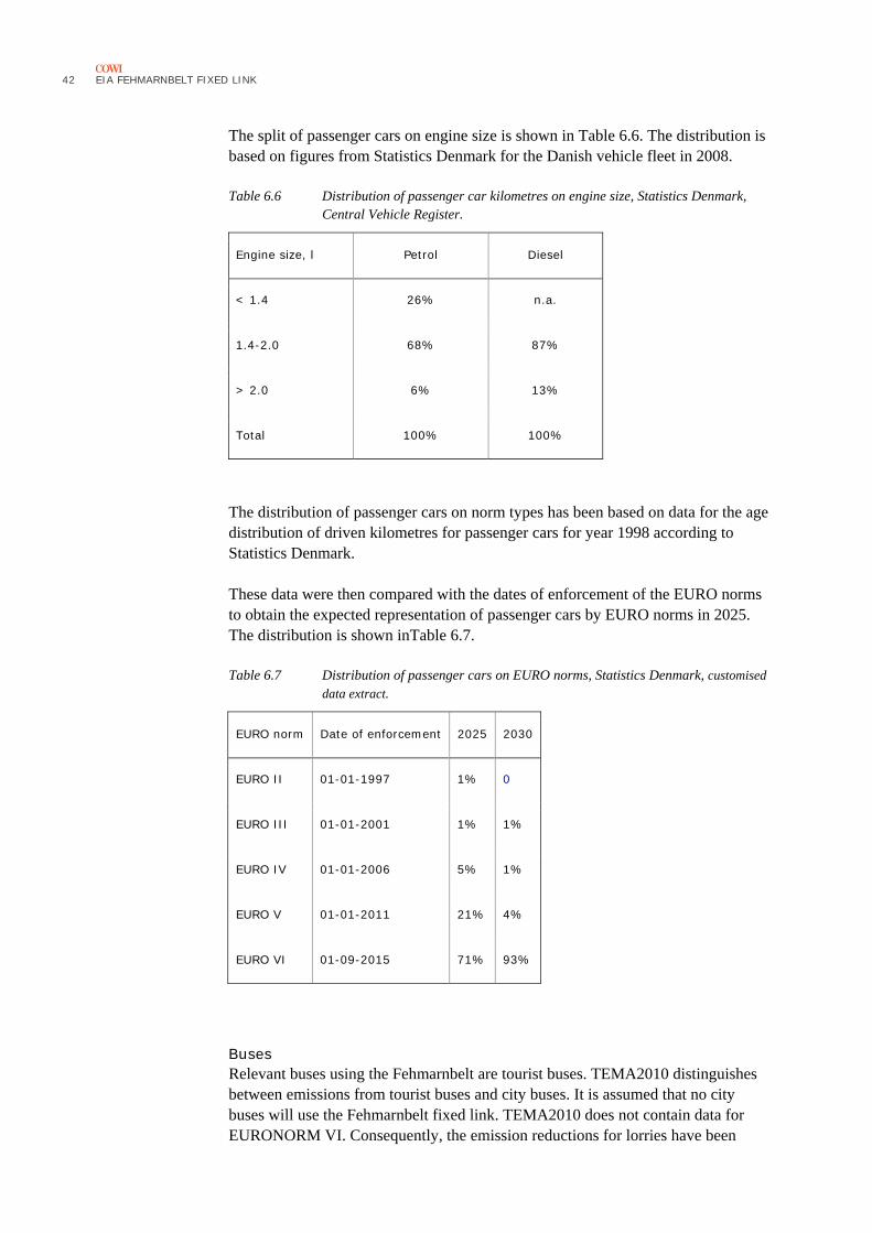
The split of passenger cars on engine size is shown in Table 6.6. The distribution is based on figures from Statistics Denmark for the Danish vehicle fleet in 2008.
Table 6.6 Distribution of passenger car kilometres on engine size, Statistics Denmark, Central Vehicle Register.
Engine size, l Petrol Diesel
< 1.4 26% n.a.
1.4-2.0 68% 87%
> 2.0 6% 13%
Total 100% 100%
The distribution of passenger cars on norm types has been based on data for the age distribution of driven kilometres for passenger cars for year 1998 according to Statistics Denmark.
These data were then compared with the dates of enforcement of the EURO norms to obtain the expected representation of passenger cars by EURO norms in 2025. The distribution is shown inTable 6.7.
Table 6.7 Distribution of passenger cars on EURO norms, Statistics Denmark, customised
data extract.
EURO norm Date of enforcement 2025 2030
EURO II 01-01-1997 1% 0
EURO III 01-01-2001 1% 1%
EURO IV 01-01-2006 5% 1%
EURO V 01-01-2011 21% 4%
EURO VI 01-09-2015 71% 93%
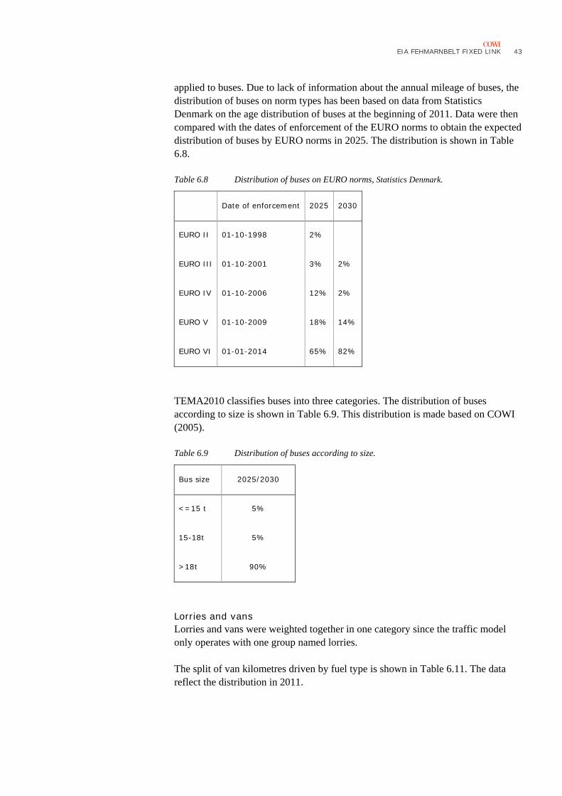
Buses Relevant buses using the Fehmarnbelt are tourist buses. TEMA2010 distinguishes between emissions from tourist buses and city buses. It is assumed that no city buses will use the Fehmarnbelt fixed link. TEMA2010 does not contain data for EURONORM VI. Consequently, the emission reductions for lorries have been
EIA FEHMARNBELT FIXED LINK
43
applied to buses. Due to lack of information about the annual mileage of buses, the distribution of buses on norm types has been based on data from Statistics Denmark on the age distribution of buses at the beginning of 2011. Data were then compared with the dates of enforcement of the EURO norms to obtain the expected distribution of buses by EURO norms in 2025. The distribution is shown in Table 6.8.
Table 6.8 Distribution of buses on EURO norms, Statistics Denmark.
Date of enforcement 2025 2030
EURO II 01-10-1998 2%
EURO III 01-10-2001 3% 2%
EURO IV 01-10-2006 12% 2%
EURO V 01-10-2009 18% 14%
EURO VI 01-01-2014 65% 82%
TEMA2010 classifies buses into three categories. The distribution of buses according to size is shown in Table 6.9. This distribution is made based on COWI (2005).
Table 6.9 Distribution of buses according to size.
Bus size 2025/2030
<=15 t 5%
15-18t 5%
>18t 90%
Lorries and vans Lorries and vans were weighted together in one category since the traffic model only operates with one group named lorries.
The split of van kilometres driven by fuel type is shown in Table 6.11. The data reflect the distribution in 2011.
44 EIA FEHMARNBELT FIXED LINK
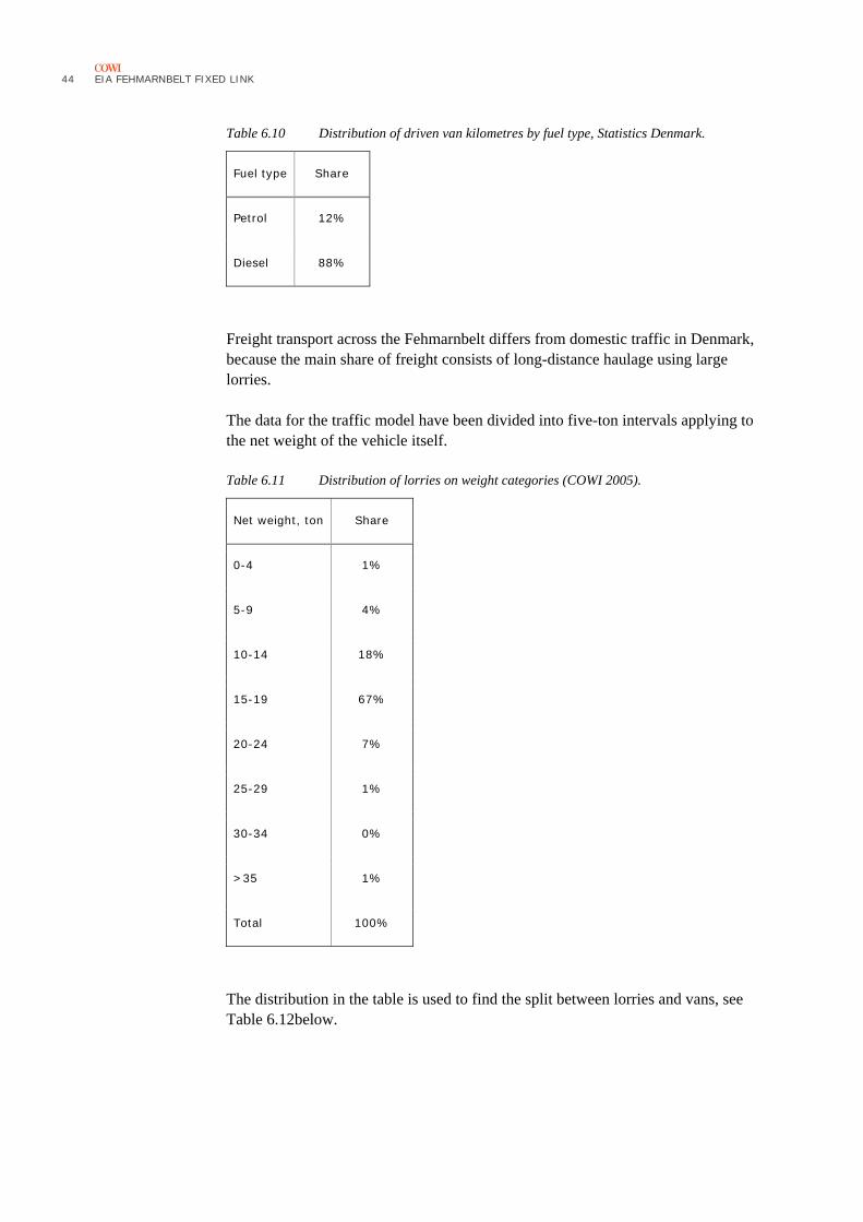
Table 6.10 Distribution of driven van kilometres by fuel type, Statistics Denmark.
Fuel type Share
Petrol 12%
Diesel 88%
Freight transport across the Fehmarnbelt differs from domestic traffic in Denmark, because the main share of freight consists of long-distance haulage using large lorries.
The data for the traffic model have been divided into five-ton intervals applying to the net weight of the vehicle itself.
Table 6.11 Distribution of lorries on weight categories (COWI 2005).
Net weight, ton Share
0-4 1%
5-9 4%
10-14 18%
15-19 67%
20-24 7%
25-29 1%
30-34 0%
>35 1%
Total 100%
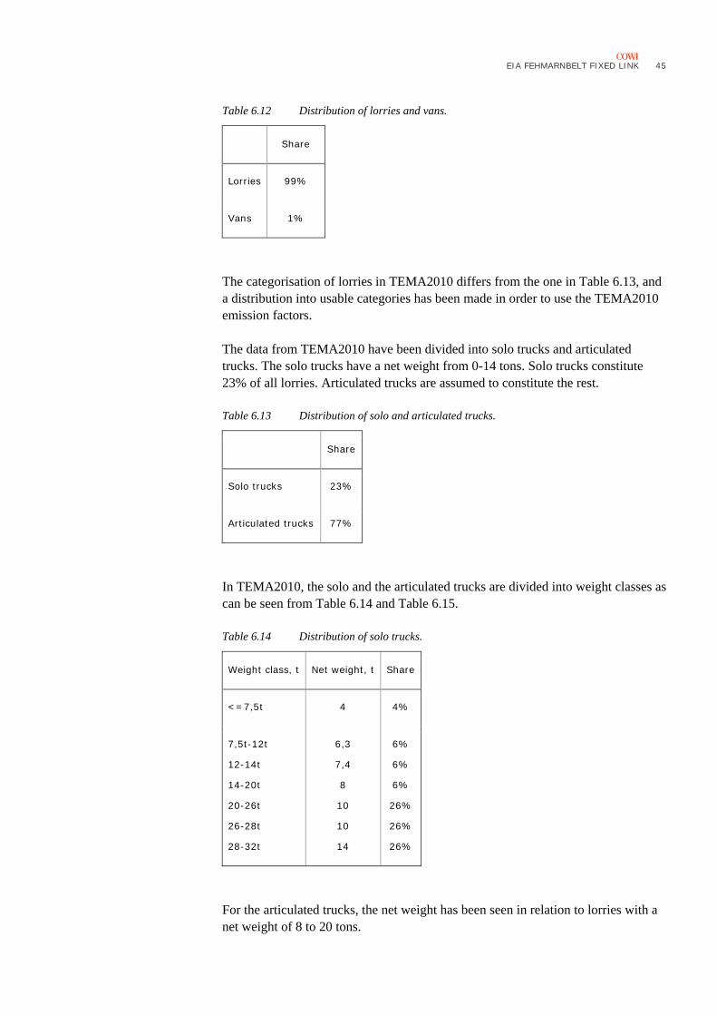
The distribution in the table is used to find the split between lorries and vans, see Table 6.12below.
EIA FEHMARNBELT FIXED LINK
45
Table 6.12 Distribution of lorries and vans.
Share
Lorries 99%
Vans 1%
The categorisation of lorries in TEMA2010 differs from the one in Table 6.13, and a distribution into usable categories has been made in order to use the TEMA2010 emission factors.
The data from TEMA2010 have been divided into solo trucks and articulated trucks. The solo trucks have a net weight from 0-14 tons. Solo trucks constitute 23% of all lorries. Articulated trucks are assumed to constitute the rest.
Table 6.13 Distribution of solo and articulated trucks.
Share
Solo trucks 23%
Articulated trucks 77%
In TEMA2010, the solo and the articulated trucks are divided into weight classes as can be seen from Table 6.14 and Table 6.15.
Table 6.14 Distribution of solo trucks.
Weight class, t Net weight, t Share
<=7,5t 4 4%
7,5t-12t
12-14t
14-20t
20-26t
26-28t
28-32t
6,3
7,4
8
10
10
14
6%
6%
6%
26%
26%
26%
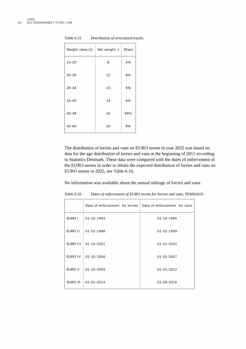
For the articulated trucks, the net weight has been seen in relation to lorries with a net weight of 8 to 20 tons.
46 EIA FEHMARNBELT FIXED LINK
Table 6.15 Distribution of articulated trucks.
Weight class,(t) Net weight, t Share
14-20 8 4%
20-28 12 6%
28-34 13 6%
34-40 14 6%
40-48 16 69%
50-60 20 8%
The distribution of lorries and vans on EURO norms in year 2025 was based on data for the age distribution of lorries and vans at the beginning of 2011 according to Statistics Denmark. These data were compared with the dates of enforcement of the EURO norms in order to obtain the expected distribution of lorries and vans on EURO norms in 2025, see Table 6.16.
No information was available about the annual mileage of lorries and vans.
Table 6.16 Dates of enforcement of EURO norms for lorries and vans, TEMA2010.
Date of enforcement for lorries Date of enforcement for vans
EURO I 01-10-1993 01-10-1995
EURO II 01-01-1998 01-01-1999
EURO III 01-10-2001 01-01-2002
EURO IV 01-10-2006 01-01-2007
EURO V 01-10-2009 01-01-2012
EURO VI 01-01-2014 01-09-2016
EIA FEHMARNBELT FIXED LINK
47
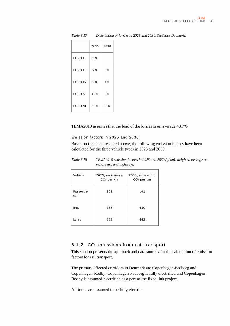
Table 6.17 Distribution of lorries in 2025 and 2030, Statistics Denmark.
2025 2030
EURO II 3%
EURO III 2% 3%
EURO IV 2% 1%
EURO V 10% 3%
EURO VI 83% 93%
TEMA2010 assumes that the load of the lorries is on average 43.7%.
Emission factors in 2025 and 2030 Based on the data presented above, the following emission factors have been calculated for the three vehicle types in 2025 and 2030.
Table 6.18 TEMA2010 emission factors in 2025 and 2030 (g/km), weighted average on motorways and highways.
Vehicle 2025, emission g CO2 per km
2030, emission g CO2 per km
Passenger car
161 161
Bus 678 680
Lorry 662 662
6.1.2 CO2 emissions from rail transport This section presents the approach and data sources for the calculation of emission factors for rail transport.
The primary affected corridors in Denmark are Copenhagen-Padborg and Copenhagen-Rødby. Copenhagen-Padborg is fully electrified and Copenhagen-Rødby is assumed electrified as a part of the fixed link project.
All trains are assumed to be fully electric.
48 EIA FEHMARNBELT FIXED LINK
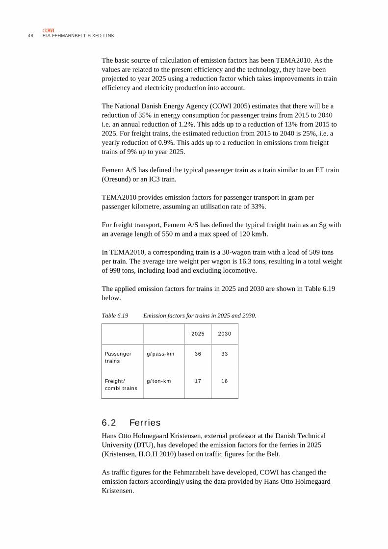
The basic source of calculation of emission factors has been TEMA2010. As the values are related to the present efficiency and the technology, they have been projected to year 2025 using a reduction factor which takes improvements in train efficiency and electricity production into account.
The National Danish Energy Agency (COWI 2005) estimates that there will be a reduction of 35% in energy consumption for passenger trains from 2015 to 2040 i.e. an annual reduction of 1.2%. This adds up to a reduction of 13% from 2015 to 2025. For freight trains, the estimated reduction from 2015 to 2040 is 25%, i.e. a yearly reduction of 0.9%. This adds up to a reduction in emissions from freight trains of 9% up to year 2025.
Femern A/S has defined the typical passenger train as a train similar to an ET train (Oresund) or an IC3 train.
TEMA2010 provides emission factors for passenger transport in gram per passenger kilometre, assuming an utilisation rate of 33%.
For freight transport, Femern A/S has defined the typical freight train as an Sg with an average length of 550 m and a max speed of 120 km/h.
In TEMA2010, a corresponding train is a 30-wagon train with a load of 509 tons per train. The average tare weight per wagon is 16.3 tons, resulting in a total weight of 998 tons, including load and excluding locomotive.
The applied emission factors for trains in 2025 and 2030 are shown in Table 6.19 below.
Table 6.19 Emission factors for trains in 2025 and 2030.
2025 2030
Passenger trains
g/pass-km 36 33
Freight/ combi trains
g/ton-km 17 16
6.2 Ferries Hans Otto Holmegaard Kristensen, external professor at the Danish Technical University (DTU), has developed the emission factors for the ferries in 2025 (Kristensen, H.O.H 2010) based on traffic figures for the Belt.
As traffic figures for the Fehmarnbelt have developed, COWI has changed the emission factors accordingly using the data provided by Hans Otto Holmegaard Kristensen.
EIA FEHMARNBELT FIXED LINK
49
The ferry routes Rødby-Puttgarden, Trelleborg-Rostock and Gedser-Rostock are included.
The ferry route distances are approximately 50 km for Gedser-Rostock and approximately 150 km for Trelleborg-Rostock compared to approximately 19 km for Rødby-Puttgarden.
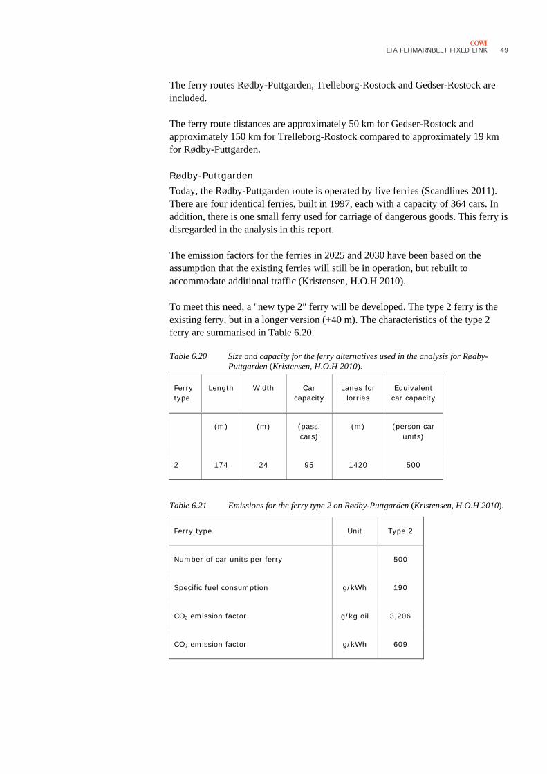
Rødby-Puttgarden Today, the Rødby-Puttgarden route is operated by five ferries (Scandlines 2011). There are four identical ferries, built in 1997, each with a capacity of 364 cars. In addition, there is one small ferry used for carriage of dangerous goods. This ferry is disregarded in the analysis in this report.
The emission factors for the ferries in 2025 and 2030 have been based on the assumption that the existing ferries will still be in operation, but rebuilt to accommodate additional traffic (Kristensen, H.O.H 2010).
To meet this need, a "new type 2" ferry will be developed. The type 2 ferry is the existing ferry, but in a longer version (+40 m). The characteristics of the type 2 ferry are summarised in Table 6.20.
Table 6.20 Size and capacity for the ferry alternatives used in the analysis for Rødby-Puttgarden (Kristensen, H.O.H 2010).
Ferry type
Length Width Car capacity
Lanes for lorries
Equivalent car capacity
(m) (m) (pass. cars)
(m) (person car units)
2 174 24 95 1420 500
Table 6.21 Emissions for the ferry type 2 on Rødby-Puttgarden (Kristensen, H.O.H 2010).
Ferry type Unit Type 2
Number of car units per ferry 500
Specific fuel consumption g/kWh 190
CO2 emission factor g/kg oil 3,206
CO2 emission factor g/kWh 609
50 EIA FEHMARNBELT FIXED LINK
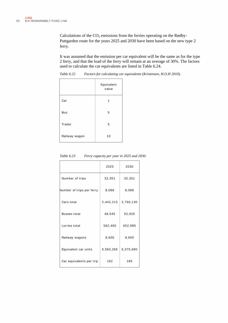
Calculations of the CO2 emissions from the ferries operating on the Rødby-Puttgarden route for the years 2025 and 2030 have been based on the new type 2 ferry.
It was assumed that the emission per car equivalent will be the same as for the type 2 ferry, and that the load of the ferry will remain at an average of 30%. The factors used to calculate the car equivalents are listed in Table 6.24.
Table 6.22 Factors for calculating car equivalents (Kristensen, H.O.H 2010).
Equivalent value
Car 1
Bus 5
Trailer 5
Railway wagon 10
Table 6.23 Ferry capacity per year in 2025 and 2030.
2025 2030
Number of trips 32,351 32,351
Number of trips per ferry 8,088 8,088
Cars total 2,442,215 2,760,130
Busses total 48,545 52,925
Lorries total 562,465 652,985
Railway wagons 8,600 8,600
Equivalent car units 5,583,265 6,375,680
Car equivalents per trip 162 185
EIA FEHMARNBELT FIXED LINK
51
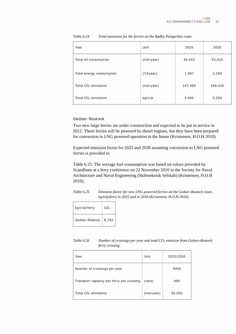
Table 6.24 Total emissions for the ferries on the Rødby-Puttgarden route.
Year Unit 2025 2030
Total oil consumption (ton/year) 46,422 53,010
Total energy consumption (TJ/year) 1,987 2,269
Total CO2 emissions (ton/year) 147,484 169,416
Total CO2 emissions kg/trip 4,605 5,258
Gedser-Rostock Two new large ferries are under construction and expected to be put in service in 2012. These ferries will be powered by diesel engines, but they have been prepared for conversion to LNG powered operation in the future (Kristensen, H.O.H 2010).
Expected emission factor for 2025 and 2030 assuming conversion to LNG powered ferries is provided in
Table 6.25. The average fuel consumption was based on values provided by Scandlines at a ferry conference on 22 November 2010 in the Society for Naval Architecture and Naval Engineering (Skibsteknisk Selskab) (Kristensen, H.O.H 2010).
Table 6.25 Emission factor for new LNG powered ferries on the Gedser-Rostock route, kg/trip/ferry in 2025 and in 2030 (Kristensen, H.O.H 2010).
kg/trip/ferry CO2
Gedser-Rostock 8,762
Table 6.26 Number of crossings per year and total CO2 emission from Gedser-Rostock ferry crossing.
Year Unit 2025/2030
Number of crossings per year 6400
Transport capacity per ferry per crossing (cars) 480
Total CO2 emissions (ton/year) 56.000
52 EIA FEHMARNBELT FIXED LINK
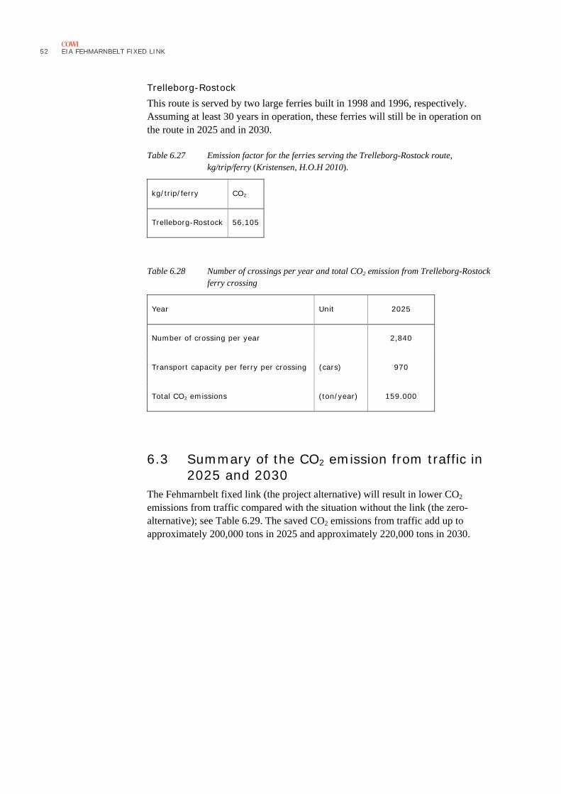
Trelleborg-Rostock This route is served by two large ferries built in 1998 and 1996, respectively. Assuming at least 30 years in operation, these ferries will still be in operation on the route in 2025 and in 2030.
Table 6.27 Emission factor for the ferries serving the Trelleborg-Rostock route, kg/trip/ferry (Kristensen, H.O.H 2010).
kg/trip/ferry CO2
Trelleborg-Rostock 56,105
Table 6.28 Number of crossings per year and total CO2 emission from Trelleborg-Rostock ferry crossing
Year Unit 2025
Number of crossing per year 2,840
Transport capacity per ferry per crossing (cars) 970
Total CO2 emissions (ton/year) 159.000
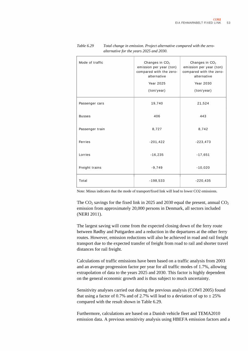
6.3 Summary of the CO2 emission from traffic in 2025 and 2030
The Fehmarnbelt fixed link (the project alternative) will result in lower CO2 emissions from traffic compared with the situation without the link (the zero-alternative); see Table 6.29. The saved CO2 emissions from traffic add up to approximately 200,000 tons in 2025 and approximately 220,000 tons in 2030.
EIA FEHMARNBELT FIXED LINK
53
Table 6.29 Total change in emission. Project alternative compared with the zero-alternative for the years 2025 and 2030.
Mode of traffic Changes in CO2 emission per year (ton) compared with the zero-
alternative
Year 2025
(ton/year)
Changes in CO2 emission per year (ton) compared with the zero-
alternative
Year 2030
(ton/year)
Passenger cars 19,740 21,524
Busses 406 443
Passenger train 8,727 8,742
Ferries -201,422 -223,473
Lorries -16,235 -17,651
Freight trains -9,749 -10,020
Total -198,533 -220,435
Note: Minus indicates that the mode of transport/fixed link will lead to lower CO2 emissions.
The CO2 savings for the fixed link in 2025 and 2030 equal the present, annual CO2 emission from approximately 20,000 persons in Denmark, all sectors included (NERI 2011).
The largest saving will come from the expected closing down of the ferry route between Rødby and Puttgarden and a reduction in the departures at the other ferry routes. However, emission reductions will also be achieved in road and rail freight transport due to the expected transfer of freight from road to rail and shorter travel distances for rail freight.
Calculations of traffic emissions have been based on a traffic analysis from 2003 and an average progression factor per year for all traffic modes of 1.7%, allowing extrapolation of data to the years 2025 and 2030. This factor is highly dependent on the general economic growth and is thus subject to much uncertainty.
Sensitivity analyses carried out during the previous analysis (COWI 2005) found that using a factor of 0.7% and of 2.7% will lead to a deviation of up to ± 25% compared with the result shown in Table 6.29.
Furthermore, calculations are based on a Danish vehicle fleet and TEMA2010 emission data. A previous sensitivity analysis using HBEFA emission factors and a
54 EIA FEHMARNBELT FIXED LINK
German vehicle fleet found only minor differences compared to the final emission calculations (COWI 2005).
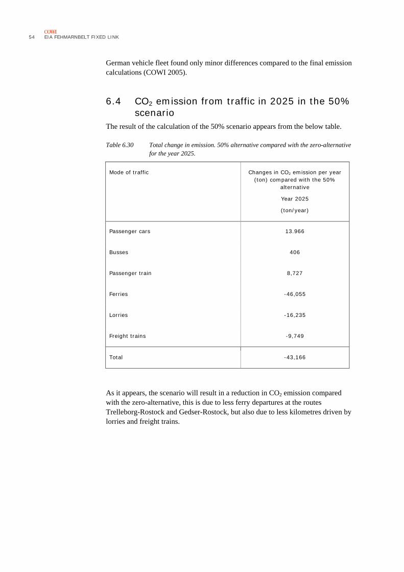
6.4 CO2 emission from traffic in 2025 in the 50% scenario
The result of the calculation of the 50% scenario appears from the below table.
Table 6.30 Total change in emission. 50% alternative compared with the zero-alternative for the year 2025.
Mode of traffic Changes in CO2 emission per year (ton) compared with the 50%
alternative
Year 2025
(ton/year)
Passenger cars 13.966
Busses 406
Passenger train 8,727
Ferries -46,055
Lorries -16,235
Freight trains -9,749
Total -43,166
As it appears, the scenario will result in a reduction in CO2 emission compared with the zero-alternative, this is due to less ferry departures at the routes Trelleborg-Rostock and Gedser-Rostock, but also due to less kilometres driven by lorries and freight trains.
EIA FEHMARNBELT FIXED LINK
55
7 Uncertainties The inventory was made at an early stage of the project, and the inputs concerning quantities of materials, use of machinery etc. were based on best estimates at this specific time of the project. Future development of the project, decisions taken by the different contractors about equipment etc. will influence the actual GHG emissions.
As mentioned earlier, the development of the three alternatives does not follow the same pace, and more information has been available for the IMT alternative. It is, however, difficult to determine how this has affected the result.
Concerning emission factors for the materials, the analysis was based on generic and average data, but the actual factors will naturally differ.
The calculations of the traffic emissions were based on a traffic analysis from 2003, and a factor of 1.7% was used to extrapolate the average annual increase in traffic volumes for all modes of transport to the years 2025 and 2030. This factor is very sensitive to the general economic growth and thus subject to much uncertainty.
Also the emission from the ferries in the future is subject to uncertainty, as it is difficult to forecast the technical development with regard to energy efficiency and also with regard to the type of ferries to be used so far ahead.
56 EIA FEHMARNBELT FIXED LINK
8 List of figures Figure 3.1 Sources to be included in the GHG emission inventory
for the construction phase of the fixed link. 11 Figure 3.2 Sources to be included in the GHG emission inventory
for the operation phase of the fixed link. 12
EIA FEHMARNBELT FIXED LINK
57
9 List of tables Table 2.1 Total changes in GHG emissions for the CSB, IMT and
BOT respectively compared with the zero-alternative in 2025. 8
Table 3.1 Emission factors used for the main materials (excl. concrete) (COWI 2011a) 14
Table 3.2 Emission factors for concrete (COWI 2011a) 14 Table 3.3 Assumptions regarding mode of transport and average
transport distance for the primary materials used in the tunnel and bridge alternatives. 15
Table 3.4 Traffic forecast figures (ADT) for road and rail traffic on the Fehmarnbelt for 2025 and 2030, zero-alternative (Femern 2011) 19
Table 4.1 Main materials to be used for the construction of the IMT and road and railway on both sides of the Belt. 22
Table 4.2 List of equipment and estimated fuel consumption (m3) during construction of the IMT and road and railway on both sides of the Belt. 24
Table 4.3 Estimated electricity consumption during construction of the IMT (kWh). 25
Table 4.4 Estimated emission of CO2 equivalents from the IMT during construction distributed on the main sources. 26
Table 4.5 Main materials to be used for the construction of the BOT and road and railway on both sides of the Belt. 26
Table 4.6 List of equipment and estimated fuel consumption (m3) during construction of the BOT and road and railway on both sides of the belt. 27
Table 4.7 Estimated electricity consumption during construction of the BOT (kWh). 28
Table 4.8 Estimated emission of CO2 equivalents from the BOT during construction distributed on the main sources. 29
Table 4.9 Main materials to be used for the construction of the CSB and road and railway on both sides of the Belt. 29
Table 4.10 List of equipment and estimated fuel consumption (m3) during construction of the CSB and road and railway on both sides of the Belt. 31
Table 4.11 Estimated electricity consumption during construction of the CSB (kWh). 32
58 EIA FEHMARNBELT FIXED LINK
Table 4.12 Estimated CO2 contribution from the CSB during construction distributed on the main sources. 32
Table 5.1 Annual electricity consumption (kWh/year) during operation of the IMT. 34
Table 5.2 Main material used for maintenance and replacement during operation of the IMT. 35
Table 5.3 Electricity consumption per year (kWh/year) during operation of the IMT. 36
Table 5.4 Main material used for maintenance and replacement during operation of the CSB. 36
Table 6.1 Distances driven between Denmark/Scandinavia and the Continent, 2015, million m/year, Case B (COWI 2005). 38
Table 6.2 Distances driven between Denmark/Scandinavia and the Continent, 2025, million km/year. 39
Table 6.3 Distances driven between Denmark/Scandinavia and the Continent, 2030, million km/year. 39
Table 6.4 Assumed vehicle speed on highways and motorways. 40 Table 6.5 Distribution of passenger car kilometres on fuel types in
2025 and 2030, (NERI 2009). 41 Table 6.6 Distribution of passenger car kilometres on engine size,
Statistics Denmark, Central Vehicle Register. 42 Table 6.7 Distribution of passenger cars on EURO norms,
Statistics Denmark, customised data extract. 42 Table 6.8 Distribution of buses on EURO norms, Statistics
Denmark. 43 Table 6.9 Distribution of buses according to size. 43 Table 6.10 Distribution of driven van kilometres by fuel type,
Statistics Denmark. 44 Table 6.11 Distribution of lorries on weight categories (COWI 2005). 44 Table 6.12 Distribution of lorries and vans. 45 Table 6.13 Distribution of solo and articulated trucks. 45 Table 6.14 Distribution of solo trucks. 45 Table 6.15 Distribution of articulated trucks. 46 Table 6.16 Dates of enforcement of EURO norms for lorries and
vans, TEMA2010. 46 Table 6.17 Distribution of lorries in 2025 and 2030, Statistics
Denmark. 47 Table 6.18 TEMA2010 emission factors in 2025 and 2030 (g/km),
weighted average on motorways and highways. 47 Table 6.19 Emission factors for trains in 2025 and 2030. 48 Table 6.20 Size and capacity for the ferry alternatives used in the
analysis for Rødby-Puttgarden (Kristensen, H.O.H 2010). 49
Table 6.21 Emissions for the ferry type 2 on Rødby-Puttgarden (Kristensen, H.O.H 2010). 49
Table 6.22 Factors for calculating car equivalents (Kristensen, H.O.H 2010). 50
Table 6.23 Ferry capacity per year in 2025 and 2030. 50 Table 6.24 Total emissions for the ferries on the Rødby-Puttgarden
route. 51
EIA FEHMARNBELT FIXED LINK
59
Table 6.25 Emission factor for new LNG powered ferries on the Gedser-Rostock route, kg/trip/ferry in 2025 and in 2030 (Kristensen, H.O.H 2010). 51
Table 6.26 Number of crossings per year and total CO2 emission from Gedser-Rostock ferry crossing. 51
Table 6.27 Emission factor for the ferries serving the Trelleborg-Rostock route, kg/trip/ferry (Kristensen, H.O.H 2010). 52
Table 6.28 Number of crossings per year and total CO2 emission from Trelleborg-Rostock ferry crossing 52
Table 6.29 Total change in emission. Project alternative compared with the zero-alternative for the years 2025 and 2030. 53
Table 6.30 Total change in emission. 50% alternative compared with the zero-alternative for the year 2025. 54
60 EIA FEHMARNBELT FIXED LINK
10 References COWI 2005: The Danish Ministry of Transport and Energy (2005): Fixed Link across the Fehmarn Belt - Effect on Emissions to Air. For Danish Ministry of Transport and Energy and Bundesministerium für Verkehr, Bau- und Wohnungswesen by COWI in cooperation with DMU. Financially supported by European Commission through the TEN-T programme. March 2005.
COWI 2010; Discussion with Henrik Duer, Senior Project manager, COWI.
COWI 2011a: CO2 Emission factors for the CO2 inventory.
DMU 2011; (http://www.dmu.dk/luft/emissioner/greenhouse_gases/)
EMEP/EEA 2010: EMEP/EEA emission inventory guidebook 2009, updated June 2010; Non-road mobile sources and machinery.
ENS 2011a: Energistyrelsens standardfaktorer for brændværdier og CO2-emissioner, 2010. http://www.ens.dk/da-DK/KlimaOgCO2/CO2Kvoter/produktionsenheder/co2_rapportering/Sider/Forside.aspx
ENS 2011b: Energistyrelsen, Forudsætninger for samfundsøkonomiske analyser på energiområdet, April 2011.
FTC 2003a: Fehmarnbelt Traffic Consortium: Fehmarn Belt Forecast 2002, Final report, April 2003.
FTC 2003b: Fehmarn Belt Forecast 2002; Reference Cases, Supplement to Final Report of April 2003 and November 2003.
Femern A/S 2011a: Traffic forecast for environmental calculations for the Fehmarnbelt fixed link and for the zero case (continued ferry service), 20 October 2011.
Femern A/S 2011b: Mail of 18 January 2011 from Henrik Bay re. emission factors for concrete.
EIA FEHMARNBELT FIXED LINK
61
ISO14040: DS/EN 14040:2008: Miljøledelse - Livscyklusvurdering principper og struktur.
Kristensen, H.O.H 2010: Hans Otto Holmegaard Kristensen, Consulting Naval Architect and senior researcher: Emissions for the ferry routes: 1) Rødby - Puttgarden, 2) Gedser - Rostock and 3) Trelleborg - Rostock, Version 2010.12.12 including Excel files.
NERI 2009;NERI Technical Report No. 703 (2009), Projection of Green house gas emission 2007-2025.
NERI 2011; NERI Technical Report No. 827, Denmark’s National Inventory Report 2011; Emission Inventories 1990-2009 – Submitted under the United Nations Framework Convention on Climate Change and the Kyoto Protocol.
Scandlines 2009: FB- Scandlines meeting minutes with answers, mail received from Toto Ringberg 3/11/2009.
Scandlines 2011: Scandlines webpage information about fleet 2011; http://minreklame.ipapercms.dk/Bordershop/Faerger/8969x1296724679/
TEMA2010: The Danish Ministry of Transport, A model to calculate emissions from transport based on transport method, route and distance. http://www.trm.dk/da/publikationer/2010/tema+2010/
WRI 2004; WORLD RESOURCES INSTITUTE; The Greenhouse Gas Protocol; A Corporate Accounting and Reporting Standard.